Heterodyne Near Field Speckles: from laser light to X-rays

Figures & data

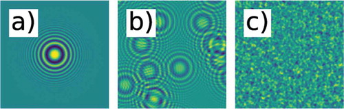
Figure 1. A sketch of the self-referencing (heterodyne) layout. The weak spherical waves scattered by a random ensemble of spheres with diameter $d$ interfere with the intense trans-illuminating beam having diameter $D$. The intensity distribution resulting from this self-referencing interference is observed at a distance $z$ downstream the sample

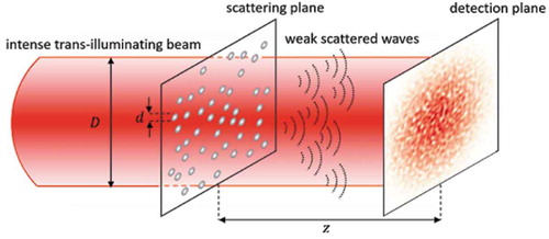
Figure 2. Heterodyne speckles arise from the sum on an intensity basis of many equal single-particle interference patterns simply formed as in-line holograms of the scattering particles. Results of numerical computations obtained for (a) $N=1$, (b) $N=30$ and (c) $N={10}^5$

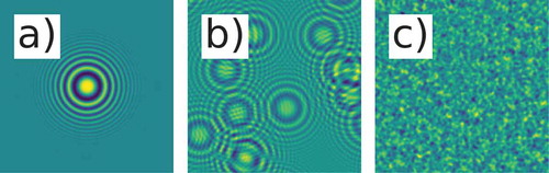
Figure 3. (a) Scattering layout and (b) Fourier Optics approach to Heterodyne Near Field Speckles. Each Fourier component with wave vector q of heterodyne speckles arises from the interference of the intense trans-illuminating beam (thicker arrows) with the faint plane waves (thinner arrows) scattered by the sample along the symmetric wave vectors ±q

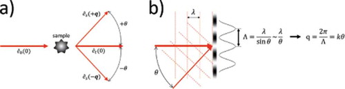
Figure 4. Heterodyne Near Field Speckles obtained with coherent light from ensembles of particles with average diameter (a,c) $d=5$ $\mu$m and (b,d) $d=10$ $\mu$m at two different distances (a,b) $z_1=1$ mm and (c,d) $z_2=2$ mm downstream the sample. Each square is 150 × 150 $\mu$m${ }^2$ in real space. The average speckle size does not vary with $z$ and it matches the size of the scatterers

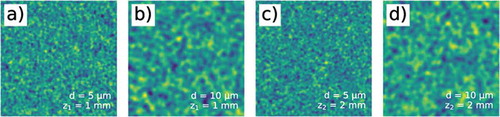
Figure 5. (a) Fourier Optics approach and (b) direct space approach to (c) the effects of Bragg-like scattering from a 3D sample on the Talbot oscillations. The Talbot oscillations are reported as a function of the reduced Fourier wave vector $q/q_{3D}$ (see text for a definition of $q_{3D}$). From plot (a), the density fluctuations occurring within each thin layer of randomly displaced particles are decomposed into Fourier modes. Each Fourier mode acts as a thin sinusoidal phase grating scattering a pair of correlated waves at $+\mathbf{q}$ and $-\mathbf{q}$. These elementary contributions from the different $n$ layers add up with random phases $exp[i{\varphi }_j^{(+)}]$ and $exp[i{\varphi }_j^{(-)}]$ for $j=1\cdots n$ along the $+\mathbf{q}$ and $-\mathbf{q}$ directions, respectively. Their incoherent sum is effective in reducing the correlation between the emerging waves ${\hat{e}}_s(\mathbf{q})$ and ${\hat{e}}_s(-\mathbf{q})$. Parameters of simulations: $\lambda =0.1$ nm, $z=50$ cm, $l=10$ cm

Figure 6. (a) Fourier Optics approach and (b) direct space approach to (c) the effects of the finite sensor size on the Talbot oscillations. The Talbot oscillations are reported as a function of the reduced Fourier wave vector $q/q_{wo}$ (see text for a definition of $q_{wo}$). From plot (a), it can be seen that $\beta$ in Equation 10(10) $T_{wo}(q,z)=\left\{\begin{array}{cc}1+\beta (q,z)\left[T(q,z)-1\right]& q\le q_{wo}\\ 1& q>q_{wo}\end{array}\right.\beta (q,z)=\frac{L-2qz/k}{L+2qz/k},$(10) is given by $\beta =A/B$, namely the ratio between the volume of the sample that scatters correlated waves at $\pm \mathbf{q}$ and the total volume of the sample intercepted by back-propagating the sensor with finite size $L$ along the ${\mathbf{k}}_s^{(\pm )}$ directions. Parameters of simulations: $\lambda =0.1$ nm, $z=50$ cm, $L=33\mu$m

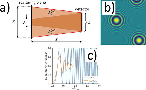
Figure 7. The phase of a partially coherent beam exhibits random (a) spatial and (f) temporal fluctuations. In (a), coherence areas elongated along the vertical direction mimic the case typically encountered with X-ray undulator radiation. (b) The instantaneous single-particle interferogram exhibits distorted fringes due to the warped phase of the incoming beam. (g) In the temporal coherence case, fringes are only radially distorted due to the azymuthal symmetry of the scattered spherical wave. At variance, the ensemble-averaged single-particle interferograms show circularly symmetric fringes whose visibility reduces according to (c) the 2D transverse coherence properties or (h) the temporal coherence properties of the incoming beam. In the former case, this implies that (d) the resulting Heterodyne Near Field Speckles are smaller along the direction of larger coherence. In the latter case, (i) speckles are rigorously isotropic. In both cases, (e,l) the corresponding power spectrum closely resembles the single-particle interference image. In particular, the envelope of the Talbot oscillations allows to access either (e) the 2D transverse coherence properties or (l) the temporal coherence properties of the incoming radiation

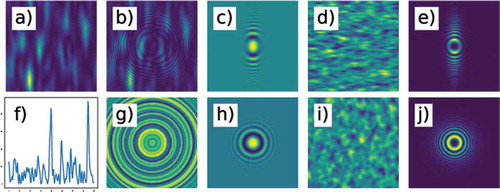
Figure 8. (a) Simulated power spectra with partially spatially coherent radiation for two different sample-detector distances. (b) The envelopes of the Talbot oscillations fit a unique master curve upon the spatial scaling

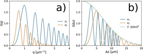
Figure 9. (a) Heterodyne Near Field Speckles, (b) radial profile of the corresponding autocorrelation functions and (c) speckle size as a function of the sample-detector distance for the case of limited spatial coherence. Plots (a) and (b) refer to z = 5 mm. The expected curve based on Equation 14 is also reported for comparison in (b). The fitted curve in (c) is obtained from Equation 15 by also including the effects from the finite size of the scatterers

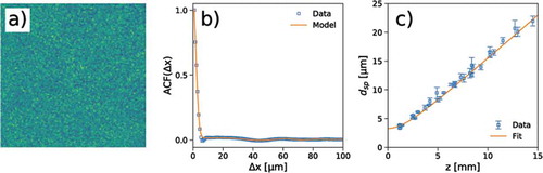
Figure 10. (a) Simulated power spectra with partially temporally coherent radiation for two different sample- detector distances. (b) The envelopes of the Talbot oscillations fit a unique master curve upon the temporal scaling. Notice how Talbot oscillations actually overlap in this case, at variance with Figure 8

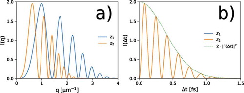
Figure 11. (a) Heterodyne Near Field Speckles, (b) radial profile of the corresponding autocorrelation functions and (c) speckle size as a function of the sample-detector distance for the case of limited temporal coherence. Plots (a) and (b) refer to the same z = 5 mm as in Figure 9. Notice how speckles become larger as the coherence properties are reduced. The expected curve based on Equation 19 is also reported for comparison in (b). The fitted curve in (c) is obtained from Equation 20 by also including the effects from the finite size of the scatterers

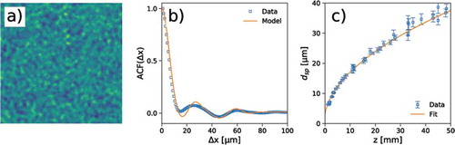
Figure 12. The three main angles that might limit the power spectrum of self-referencing speckles, hence the speckle size: the scattering angle of the particles ($\lambda /d$, blue), the angle subtended by the coherence areas (${\sigma }_{\mathrm{c}\mathrm{o}\mathrm{h}}/z$, green), the angle at which the optical path difference equals the longitudinal coherence length ($(2l_{\mathrm{c}\mathrm{o}\mathrm{h}}/z{)}^{1/2}$, red). These three cases ultimately lay the foundation of Section 2.2, Section 3.2 and Section 3.3, respectively

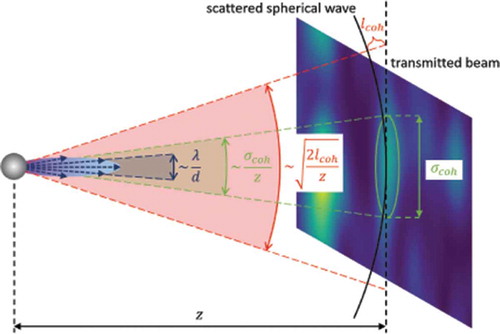
Table 1. Summary of the size of Heterodyne Near Field Speckles under different illumination conditions. The corresponding effects on power spectra are evidenced, as well as relevant examples from the published literature

	${\theta }_{\mathrm{m}\mathrm{a}\mathrm{x}}=\lambda /d$	${\theta }_{\mathrm{m}\mathrm{a}\mathrm{x}}={\sigma }_{\mathrm{c}\mathrm{o}\mathrm{h}}/z$	${\theta }_{\mathrm{m}\mathrm{a}\mathrm{x}}=(2l_{\mathrm{c}\mathrm{o}\mathrm{h}}/z{)}^{1/2}$
Speckle size	$d_{sp}=d$	$d_{sp}=\lambda z/{\sigma }_{\mathrm{c}\mathrm{o}\mathrm{h}}$	$d_{sp}=[{\lambda }^{2}z/(2l_{\mathrm{c}\mathrm{o}\mathrm{h}}){]}^{1/2}$
Scaling of power spectrum	None	$\mathrm{\Delta }\mathbf{x}=z\mathbf{q}/k$	$\mathrm{\Delta }t=z{q}^2/(2k^{2}c)$
Applications^a	Particle sizing	Spatial coherence	Temporal coherence
References	[14–24,30,31]	[28,29,32–36,39,40]	[28,29,36–38]

^aIn [25–27] (velocimetry), the speckle size is actually limited by the numerical aperture $NA$ of the collection optics. Thus, subjective speckles arise and ${\theta }_{\mathrm{m}\mathrm{a}\mathrm{x}}\sim NA$ in Equation 21(21) $d_{sp}(z)=\frac{2\pi }{q_{\mathrm{m}\mathrm{a}\mathrm{x}}(z)}=\frac{\lambda }{{\theta }_{\mathrm{m}\mathrm{a}\mathrm{x}}(z)}{\theta }_{\mathrm{m}\mathrm{a}\mathrm{x}}(z)=min\left\{\frac{\lambda }{d},\frac{{\sigma }_{\mathrm{c}\mathrm{o}\mathrm{h}}}{z},\sqrt{\frac{2l_{\mathrm{c}\mathrm{o}\mathrm{h}}}{z}}\right\}.$(21) . In [41–83] (X-ray wavefront sensing and X-ray phase-contrast imaging), both the size of the scatterers and the finite extent of the coherence areas might simultaneously play a role.

Cerbino R, Peverini L, Potenza MAC, et al. X-ray-scattering information obtained from near-field speckle. Nat. Phys. 2008;4:238–243.

 Web of Science ®Google Scholar

Lu X, Mochrie SGJ, Narayanan S, et al. X-ray near-field speckle: implementation and critical analysis. J. Synchrotron Rad. 2011;18:823–834.

 PubMed Web of Science ®Google Scholar

Siano M, Paroli B, Chiadroni E, et al. Measurement of power spectral density of broad-spectrum visible light with heterodyne near field scattering and its scalability to betatron radiation. Opt Express. 2015;23:32888–32896.

 PubMed Web of Science ®Google Scholar

Siano M, Paroli B, Chiadroni E, et al., Note: Nanosecond LED-based source for optical modeling of scintillators illuminated by partially coherent X-ray radiation. Rev. Sci. Instrum. 87 (2016), p.126104.

 PubMed Web of Science ®Google Scholar

Mazzoni S, Roncarolo F, Trad G, et al., Proc. of IBIC. Shanghai, China, 2018.

 Google Scholar

Siano M, Paroli B, Potenza MAC, et al., Proc. of IBIC. Malmo, Sweden, 2019.

 Google Scholar