Combining recorded failures and expert opinion in the development of ANN pipe failure prediction models

Figures & data

Figure 1. Failure rate by utility size and reported cause in Switzerland.

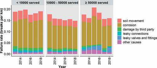
Figure 2. Pipe materials used in Swiss water distribution networks (SVGW, 2016).

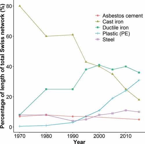
Table 1. Literature on the use of ANN for municipal pipe networks.

Reference	Inputs^1	Output	Models^2	ANN development	Performance comparison	Case study
Sacluti (1999)	11, 12	Area failure density	CI	MLP (1 hidden layer) with BEP. Coefficient of determination (R^2) used as performance criteria.	Number and data form of inputs varied.	22-yr dataset from Edmonton, CAN
Christodoulou et al. (2003); Christodoulou and Deligianni (2010)	1, 2, 4, 5, 33	Time to failure (days)	G	MLP (1 hidden layer). ANN integrated into a neuro-fuzzy decision framework.	1 vs. 2 hidden layers compared	10-yr dataset from New York City and Limassol, Cyprus
Ahn et al. (2005)	4, 11, 12, 13, 14	Network pipe failures	G	MLP (2 hidden layers) with BEP. Mean absolute error (MAE) used as performance criteria.	Not included	9-yr dataset from Seoul, South Korea
Najafi and Kulandaivel (2005)	1, 2, 4, 7, 15, 16, 17	Sewer pipe condition scale	G	MLP (1 hidden layer) with BEP. Root mean squared error (RMSE) used as performance criteria.	Number of nodes in hidden layer altered	Dataset from Atlanta, USA
Al-Barqawi and Zayed (2006)	1, 4, 6, 7, 15, 18, 19, 20,	Water pipe condition scale	G	MLP (1 hidden layer) with BEP. MAE, RMSE, average invalidity percent (AIP), and average validity percent (AVP) used as performance criteria	Not done	Dataset from three Canadian municipalities (Moncton, NB; Longueuil, QC; London, ON)
Achim et al. (2007)	1, 2, 3, 7, 21	Failure rate	G	MLP (2 hidden layers) with BEP. Coefficient of determination (R^2) used as performance criteria.	Inputs varied, number of hidden nodes varied	5-yr dataset from Victoria, Australia
Geem et al. (2007)	1, 4, 6, 7, 10, 15, 21, 22, 23, 30	Pipe condition index	G	MLP (1 hidden layer) with BEP. Coefficient of determination (R^2) used as performance criteria.	Not done	Data from water utility in South Korea
Tabesh et al. (2009)	1, 2, 7, 10, 15	Failure rate	G	MLP (1 and 2 hidden layers) with BEP. Index of agreement (IOA) and RMSE used as performance criteria.	Number of nodes in hidden layer	Data from city in Iran
Amaitik and Amaitik (2010)	7, 10, 15, 24, 25, 26, 27	Number of broken wires in PCCP	PCCP	MLP (2 hidden layers) with BEP. Coefficient of determination (R^2) used as performance criteria.	Not done	10-yr dataset of monitoring data from non-destructive techniques (NDT) of Libyan water network
Jafar, Shahrour, & Juran, (2007, 2010)	1, 2, 5, 6, 7, 8, 9, 31	Number of failures	P, AC, M, NoF, G	MLP (1 hidden layer). Coefficient of determination (R^2) and average squared error (ASE) used as performance criteria.	Not done	14-yr dataset of medium-sized city in Northern France.
Asnaashari et al. (2013)	1, 2, 4, 5, 6, 7, 29, 30	Failure rate	G	MLP (1 hidden layer). Coefficient of determination (R^2) and average squared error (ASE) used as performance criteria. 50:25:25 data split used.	Neurons in hidden layer. ANN compared to multiple linear regression (MLR)	20-yr dataset from Etobicoke, CAN.
Harvey et al. (2014)	1, 2, 3, 5, 6, 29, 30	Time to failure	AS, CI, DI	MLP (1 hidden layer). Correlation coefficient (R) and sum squared error (SSE) used as performance criteria. 70:15:15 data split used.	Initial weights and neurons in hidden layer	43-yr dataset from Scarborough, CAN.
Kutyłowska, (2015, 2017)	1, 2, 3, 4, 5, 17,32	Network failure rate per pipe type	DP, SL, G	Radial Basis Functions ANN (7-4-3) and MLP ANN (7–14-3) compared. 50:25:25 data split used in training phases. Absolute relative error and correlation coefficient used for performance.	Activation functions and ANN types	14 yr dataset from a city in Poland
Kerwin et al. (2018)	1, 3, 4, 5, 6, 10, 34	Time to failure	G, CI, DI	MLP (1 hidden layer) with BEP. 80:10:10 split	Material-specific compared to generalized model with MSE.	48-yr dataset from medium-sized utility (over 1000 km buried pipe)
Snider and McBean (2018)	1, 2, 3, 5, 6, 10, 28, 29, 34	Time to failure	DI	Developed in R using nnet package. 10-fold cross-validation repeated 3x.	Decision-tree based models (gradient boosting, random forest) compared to ANN	57-yr dataset from large North American utility
Sattar et al. (2019)	1, 2, 3, 5, 6, 28, 29	Failure rate	AC, CI, DI	MLP (one hidden layer) with extreme learning machine training algorithm instead of BEP	Four training algorithms compared	59-yr dataset from Scarborough, CAN

1. 1 – Diameter, 2 – Length, 3 – Construction year, 4 – Material, 5 – Number of previous failures, 6 – Soil type, 7 – Age at failure, 8 – Location underground, 9 – Pressure variation, 10 – Pressure head, 11 – Various air temperature measurements, 12 – Various water temperature measurements, 13 – Various soil temperature measurements, 14- Ratio of metered water, 15- Burial depth, 16 – Pipe slope (sewer), 17 – Pipe type, 18 – Road surface, 19 – Pipe failure rate, 20 – Hazen Williams coefficient, 21 – Geographical coordinates, 21 – Electric recharge, 22 – Bedding condition, 23 – Number of road lanes, 24 – Time between failures, 25 – Soil resistivity, 26 – Soil density, 27 – Wire characteristics, 28 – Cathodic protection, 29 – Cement mortar lining, 30 – Presence of pipe surface coating, 31 – Pipe thickness, 32 – Number of service lines, 33 – Various traffic parameters, 34 – Zoning

2. AC – Asbestos cement, CI – Cast iron, DI – Ductile iron, DP – Distribution pipes, G – Global/general, M – Metallic, NoF – Number of failures (high/low), P – plastic, PCCP – Pre-stressed concrete cylinder pipe (PCCP), SL – Service lines

Figure 3. (a) Schematic of a multi-layer perceptron (García de Soto et al., 2014); (b) Data conversion process in a perceptron (Adey et al., 2017).

Figure 4. Methodology for development of ANN failure prediction model.

Table 2. Parameters found in databases.

Parameters	Pipe database	Failure database	GIS database
Unique ID	●	●
Material type	●	●
Diameter	●	●
Construction year	●	●
Length	●
Number of previous failures	●
Failure date		●
Failure type		●
Closest address to failure		●
Zoning			●
Soil type			●

Table 3. Pipe database summarizing table.

Parameter	Pipe material
	CI	DI1	DI2	DI3	PE	Steel	AC
Number of pipes	1570	1957	1258	1152	15190	1002	625
Build year	1903–1969	1956–1980	1981–1993	1985–2015	1961–2015	1933–2015	1934–1996
Average age	67	45.9	33.2	12.7	20.2	53.2	49.5
Average pipe length (m)	109.1	144.4	116.4	97.9	25.2	86.1	164.1
Total pipe length (km)	171.2	282.6	146.4	112.8	382.1	86.3	102.5
Percentage of network in pipe length (%)	11.5	19.0	9.9	7.6	25.7	5.8	6.9
Diameter (mm)	40–500	40–600	50–600	30–500	20–450	15–800	60–700
Percentage of pipes – no failure (%)	62.9	64.8	82.5	98.1	98.5	89.5	79.2
Percentage of pipes – at least one failure (%)	37.1	35.2	17.5	1.9	1.5	10.5	20.8

Table 4. Failure database summarizing table.

Parameter	Pipe material
	CI	DI1	DI2	DI3	PE	Steel	AC
Number of failures	1992	1791	274	49	132	204	180
Unique pipe IDs	1274	1299	241	45	125	146	151
Pipes with only one failure (%)	66.7	76.4	85.4	88.8	92.8	78.1	81.5
Build year	1900–1969	1958–1980	1981–1993	1985–2019	1963–2019	1931 − 1984	1934 − 1988
Failure year	1968–2019	1968–2019	1981–2019	1995–2019	1988–2019	1968–2019	1968–2019
Diameter (mm)	40 − 600	50–500	50–500	80–400	30–200	30–600	60–500

Figure 5. Annual recorded failures by material type.

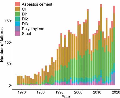
Figure 6. Annual recorded failures caused by (a) soil movement and (b) corrosion.

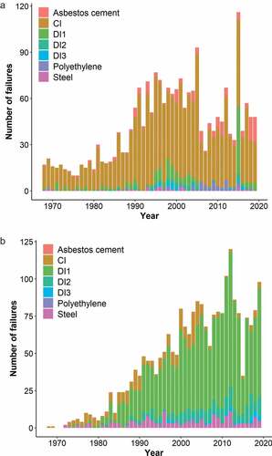
Figure 7. Average monthly failures by (a) material type; (b) reported cause of failure.

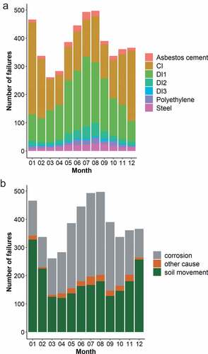
Figure 8. Comparison of time to first failure of observations (histogram) and Weibull distribution (red curve) based on expert opinion for a) asbestos cement, b) steel, c) DI1.

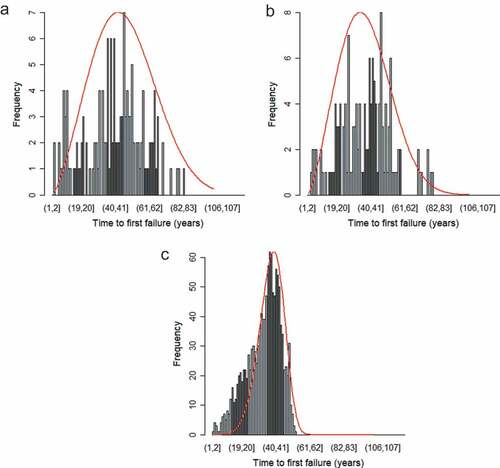
Figure 9. Distribution of time to first failure of (a) PE failures in failure database with fitted Weibull distribution (k = 1.81, λ = 65.72); (b) resulting PE failures.

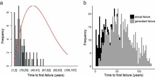
Table 5. ANN input and target parameters.

Parameter	Type	Units/Description	Training data
			Observed failures	Observed and generated failures
Total entries	Integer	Number of entries	4622	5522
Generated failures	Integer	Number of entries	0	708 (PE), 192 (DI3)
Previous failures	Integer		0–12	0–12
Diameter	Numeric	mm	30–600	30–600
Length	Numeric	m	0.4–1631.8	0.4–1631.8
Build year	Integer		1900–2019	1900–2019
Material	Binary	7 distinct categories (CI, DI1, DI2, DI3, ST, AC, PE)
Zoning	Binary	13 distinct categories based on use (e.g., residential, industrial) and population density
Soil texture	Binary	11 distinct categories based on clay, silt, sand composition
Time to failure	Numeric	Years	0–115	0–183

Figure 10. Investigation of the effect of training algorithm, scaling method and activation function on ANN model performance (scg – scaled conjugate gradient, lm: Levenberg-Marquardt).

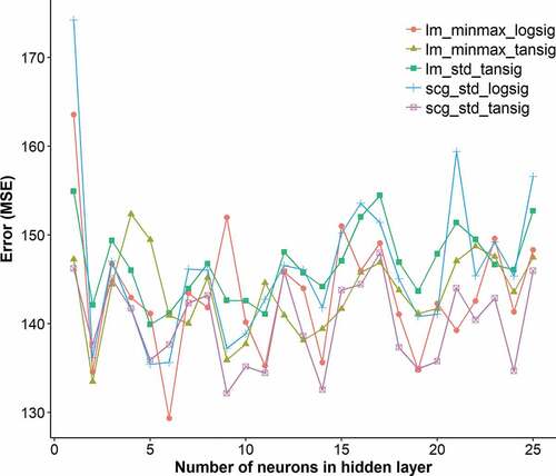
Table 6. ANN model results.

Training data	Architecture	Dataset	Instances	MSE	R
Observed failures only	35 – 11 – 1	Training	3698	137.0	0.851
		Validation	462	138.8	0.812
		Testing	462	100.0	0.882
Observed and generated failures	35 – 9 – 1	Training	4418	343.6	0.732
		Validation	552	344.4	0.703
		Testing	552	250.1	0.794

Table 7. Input importance of ANN models (only top 10 inputs of both models shown).

Input	Trained with observed failures only			Trained with observed and generated failures
	Ranking	Weight	Relative	Ranking	Weight	Relative
Number of previous failures	1	2.90	100%	1	2.34	100%
Construction year	2	1.55	53%	2	1.00	43%
Soil – silt	3	0.60	21%	5	0.22	9%
Pipe material – DI1	4	0.48	17%	7	0.14	6%
Soil – clayey silt	5	0.39	14%	6	0.18	8%
Pipe material – DI2	6	0.33	11%	11	0.13	5%
Soil – silty clay	7	0.30	10%	10	0.13	5%
Zoning – urban/village hub	8	0.24	8%	18	0.06	3%
Zoning – high density downtown	9	0.19	7%	27	0.03	1%
Zoning – residential low density	10	0.19	6%	4	0.27	11%
Pipe material – PE	11	0.18	6%	3	0.61	26%
Pipe material – DI3	14	0.15	5%	8	0.14	6%
Soil – sandy silt	21	0.07	3%	9	0.14	6%

Figure 11. (a) Scatterplot for ANN only trained with observed failures. R = 0.851; (b) Scatterplot for ANN trained with observed and generated failures. R = 0.736.

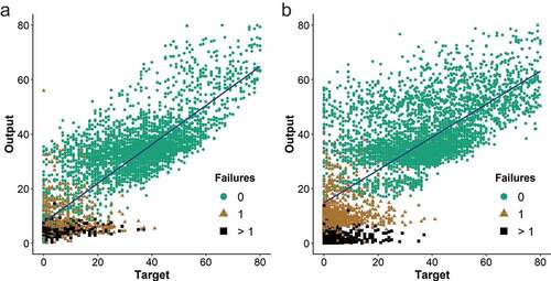
Figure 12. (a) Overall error histogram. MSE: 133.5 (ANN trained only with observed failures). MSE: 334.3 (ANN trained with observed and generated failures). (b) Error histogram for cast iron pipes. MSE: 186.2 (ANN trained only with observed failures). MSE: 204.5 (ANN trained with observed and generated failures).

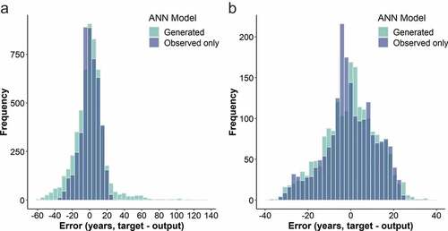
Figure 13. (a) Error histogram for DI1 pipes. MSE: 86.3 (ANN trained only with observed failures). MSE: 90.5 (ANN trained with observed and generated failures); (b) Error histogram for DI2 pipes. MSE: 94.8 (ANN trained only with observed failures). MSE: 92.9 (ANN trained with observed and generated failures).

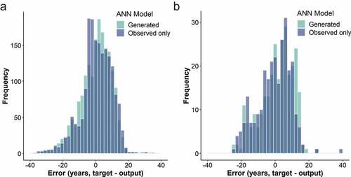
Figure 14. (a) Error histogram for DI3 pipes. MSE: 62.2 (ANN trained only with observed failures). MSE: 1260.9 (ANN trained with observed and generated failures); (b) Error histogram for PE pipes. MSE: 65.6 (ANN trained only with observed failures). MSE: 1070.9 (ANN trained with observed and generated failures).

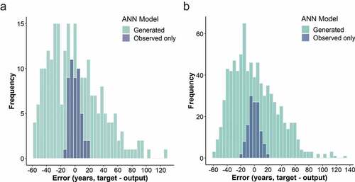
Figure 15. (a) Error histogram for asbestos cement pipes. MSE: 137.6 (ANN trained only with observed failures). MSE: 158.7 (ANN trained with observed and generated failures); (b) Error histogram for steel pipes. MSE: 142.8 (ANN trained only with observed failures). MSE: 173.1 (ANN trained with observed and generated failures).

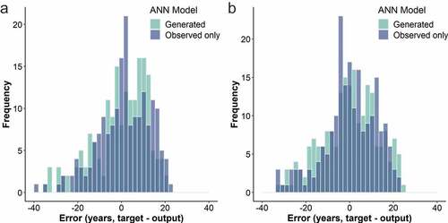
Figure 16. Time to next failure (a) using ANN model trained with only observed failures; (b) using ANN model trained with observed and generated failures.

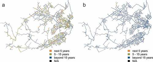
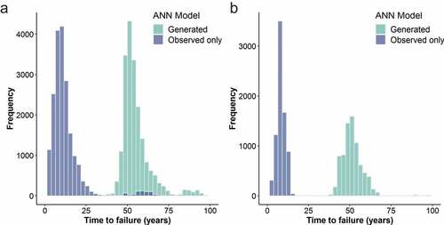
Figure 17. Distribution of time to next failure for example subnetwork for both developed ANN models for (a) PE pipes; (b) DI3 pipes.

SVGW. (2016). Statistische Erhebungen der Wasserversorgungen in der Schweiz Betriebsjahr 2015. Zürich.

 Google Scholar

Sacluti, F. R. (1999). Modelling water distribution pipe failures using artificial neural networks. Edmonton, Canada: University of Alberta.

 Google Scholar

Christodoulou, S., Aslani, P., & Vanrenterghem, A. (2003). A risk analysis framework for evaluating structural degradation of water mains in urban settings, using neurofuzzy systems and statistical modeling techniques. World Water & Environmental Resources Congress 2003. Reston, VA, USA: ASCE.

 Google Scholar

Christodoulou, S., & Deligianni, A. (2010). A neurofuzzy decision framework for the management of water distribution networks. Water Resources Management, 24(1), 139–156. doi:10.1007/s11269-009-9441-2

 Web of Science ®Google Scholar

Ahn, J., Lee, S., Lee, G., & Koo, J. (2005). Predicting water pipe breaks using neural network. Water Science and Technology: Water Supply, 5(3–4), 159–172.

 Google Scholar

Najafi, M., & Kulandaivel, G. (2005). Pipeline condition prediction using neural network models. Pipelines 2005: Optimizing Pipeline Design, Operations, and Maintenance in Today’s Economy, 767–781. https://ascelibrary.org/action/showCitFormats?doi=10.1061%2F40800%28180%2961

 Google Scholar

Al-Barqawi, H., & Zayed, T. (2006). Condition rating model for underground infrastructure sustainable water mains. Journal of Performance of Constructed Facilities, 20(2), 126–135. doi:10.1061/(ASCE)0887-3828(2006)20:2(126)

 Web of Science ®Google Scholar

Achim, D., Ghotb, F., & McManus, K. (2007). Prediction of water pipe asset life using neural networks. Journal of Infrastructure Systems, 13(1), 26–30. doi:10.1061/(ASCE)1076-0342(2007)13:1(26)

 Web of Science ®Google Scholar

Geem, Z. W., Tseng, C.-L., Kim, J., & Bae, C. (2007). Trenchless water pipe condition assessment using artificial neural network. Pipelines 2007: Advances and Experiences with Trenchless Pipeline Projects, 1–9. https://ascelibrary.org/action/showCitFormats?doi=10.1061%2F40934%28252%2926

 Google Scholar

Tabesh, M., Soltani, J., Farmani, R., & Savic, D. (2009). Assessing pipe failure rate and mechanical reliability of water distribution networks using data-driven modeling. Journal of Hydroinformatics, 11(1), 1–17. Retrieved from http://jh.iwaponline.com/content/ppiwajhydro/11/1/1.full.pdf

 Web of Science ®Google Scholar

Amaitik, N. M., & Amaitik, S. M. (2010). Prediction of pipe failures in water mains using artificial neural network models.

 Google Scholar

Jafar, R., Shahrour, I., & Juran, I. (2007). Modelling the structural degradation in water distribution systems using the artificial neural networks (ANN). Water Asset Management International, 3(3), 14–18.

 Google Scholar

Jafar, R., Shahrour, I., & Juran, I. (2010). Application of Artificial Neural Networks (ANN) to model the failure of urban water mains. Mathematical and Computer Modelling, 51(9–10), 1170–1180. doi:10.1016/j.mcm.2009.12.033

 Google Scholar

Asnaashari, A., McBean, E. A., Gharabaghi, B., & Tutt, D. (2013). Forecasting watermain failure using artificial neural network modelling. Canadian Water Resources Journal, 38(1), 24–33. doi:10.1080/07011784.2013.774153

 Web of Science ®Google Scholar

Harvey, R., McBean, E. A., & Gharabaghi, B. (2014). Predicting the timing of water main failure using artificial neural networks. Journal of Water Resources Planning and Management, 140(4), 425–434. doi:10.1061/(ASCE)WR.1943-5452.0000354

 Web of Science ®Google Scholar

Kutyłowska, M. (2015). Neural network approach for failure rate prediction. Engineering Failure Analysis, 47, 41–48. doi:10.1016/j.engfailanal.2014.10.007

 Web of Science ®Google Scholar

Kutyłowska, M. (2017). Comparison of two types of artificial neural networks for predicting failure frequency of water conduits. Periodica Polytechnica Civil Engineering, 61(1), 1–6.

 Web of Science ®Google Scholar

Kerwin, S., García de Soto, B., & Adey, T. B. (2018) Performance comparison for pipe failure prediction using artificial neural networks. Paper presented at the IALCCE 2018, Ghent, Belgium.

 Google Scholar

Snider, B., & McBean, E. A. (2018). Improving time to failure predictions for water distribution systems using extreme gradient boosting algorithm. WDSA/CCWI Joint Conference Proceedings, Kingston, Ontario, Canada.

 Google Scholar

Sattar, A. M., Ertuğrul, Ö. F., Gharabaghi, B., McBean, E. A., & Cao, J. (2019). Extreme learning machine model for water network management. Neural Computing & Applications, 31(1), 157–169. doi:10.1007/s00521-017-2987-7

 Web of Science ®Google Scholar

García de Soto, B., Adey, B. T., & Fernando, D. (2014). A process for the development and evaluation of preliminary construction material quantity estimation models using backward elimination regression and neural networks. Journal of Cost Analysis and Parametrics, 7(3), 180–218. doi:10.1080/1941658X.2014.984880

 Google Scholar

Adey, B. T., Richmond, C., & García de Soto, B. (2017). Infrastructure management 2: Evaluation tools. ETH Zurich: Course script. Infrastructure Management.

 Google Scholar