Figures & data
Figure 1. Flowchart of the data processing done. The values are output for each time step and particle.
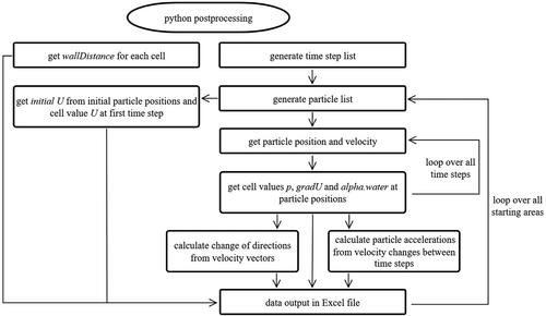
Figure 2. Section of the calculation area with a cell length of 2.0 cm. In red: Areas in which at least 80 % of the turbulent kinetic energy is simulated and less than 20 % is modelled by Sub-grid models. In blue: Areas in which more than 20 % is modelled. The white lines represent the water surface.
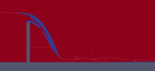
Figure 3. Initial positions of the particles of the cases with a weir height of 3 m W3T2 and W3T0 (left) and of the cases with a weir height of 4 m W4T2 and W4T0 (right). Starting areas: A1 – below the surface (red; h = 0.3 m), A2 – covering the area between A1 and A3 (green; h = 0.25–1.1 m) and A3 – above the weir crest (blue; h = 0.3 m).
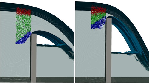
Figure 4. Slices through the computational domains of the four cases showing the hydraulic situations. Depicted in blue is the water-filled area. Starting from the top, W3T0 with a weir height of 3 m and a tailwater level of 0 m, W3T2 with a weir height of 3 m and a tailwater level of 2 m, W4T0 with a weir height of 4 m and a tailwater level of 0 m and W4T2 with a weir height of 4 m and a tailwater level of 2 m.
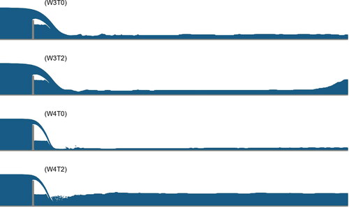
Figure 5. Sum lines and distribution of shear stress experienced by the particles. Cases W3T0 and W4T0 (left figures) have a tailwater level of 0 m, and cases W3T2 and W4T2 (right figures) of 2 m. The weir has a height of 3 m in the top row (W3T0 and W3T2) and 4 m in the bottom row (W4T0 and W4T2).
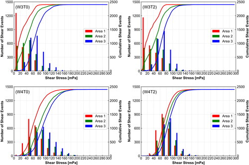
Figure 6. Sum lines and distribution of pressure changes experienced by particles. Cases W3T0 and W4T0 (left figures) have a tailwater level of 0 m, and cases W3T2 and W4T2 (right figures) of 2 m. The weir has a height of 3 m in the top row (W3T0 and W3T2) and 4 m in the bottom row (W4T0 and W4T2).
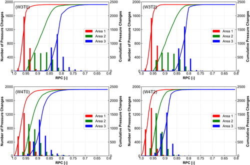
Figure 7. Sum lines and distribution of particle velocities perpendicular to the wall before recorded collisions. Cases W3T0 and W4T0 (left figures) have a tailwater level of 0 m, and cases W3T2 and W4T2 (right figures) of 2 m. The weir has a height of 3 m in the top row (W3T0 and W3T2) and 4 m in the bottom row (W4T0 and W4T2).
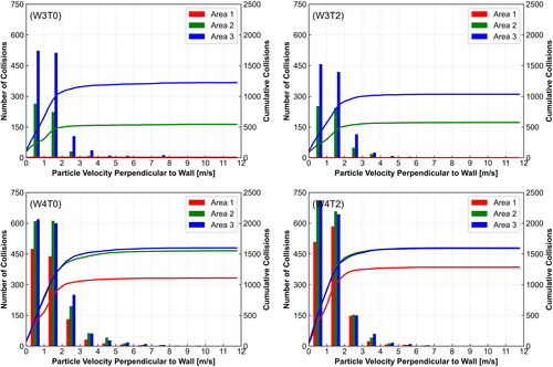
Figure 8. Number of recorded collisions divided according to the particle velocity perpendicular and parallel to the wall before the collision. From top to bottom: W3T0 (weir height 3 m, tailwater level 0 m), W3T2 (weir height 3 m and tailwater level 2 m), W4T0 (weir height 4 m and tailwater level 0 m), W4T2 (weir height 4 m and tailwater level 2 m). The first column (red) is starting area 1, the second column (green) starting area 2 and the third column (blue) starting area 3.
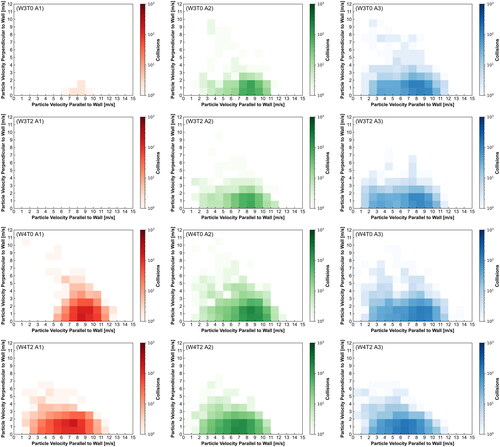
Figure 9. Locations and impact velocities of all recorded collisions of case W4T2. The velocity is plotted on the background. The cell size is visible on the bottom.
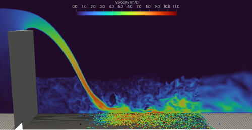
Figure 10. The geometry of the Pulverweiden weir with two segment gates, the stilling basin and two rows of baffle blocks. Headwater on the left and tailwater on the right. The red box indicates the model area.
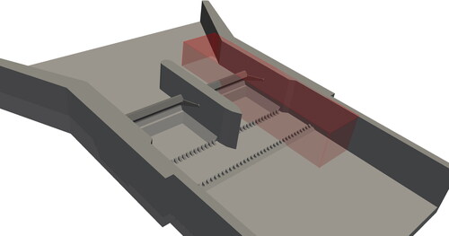
Figure 11. Section of the calculation area with a cell length of 2.0 cm. In red: Areas in which at least 80 % of the turbulent kinetic energy is simulated and less than 20 % is modelled by Sub-grid models. In blue: Areas in which more than 20 % is modelled. The white lines represent the water surface.
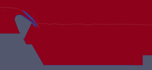
Figure 12. Initial flow conditions of the four situations considered. In the first two cases (top), the weir is operated as an overshot weir and in the two later cases (bottom), the weir is operated as an undershot weir. The water velocity is plotted on the slice.
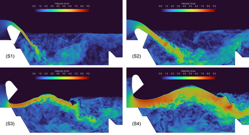
Figure 13. Sum lines of shear stress experienced by the particles. Cases S1 and S2 (top figures) are overshot situations, and cases S3 and S4 (bottom figures) are undershot situations. The discharge increases from 50 m3/s (S1) to 110 m3/s (S2 and S3) and 240 m3/s (S4).
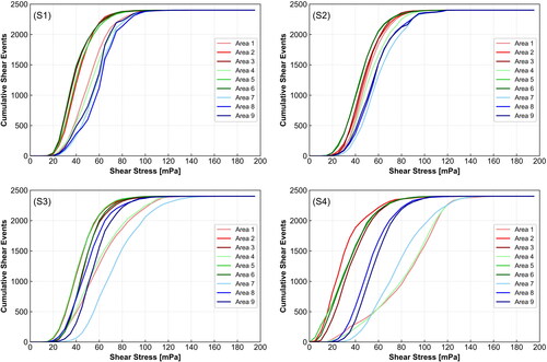
Figure 14. Sum lines of pressure changes experienced by the particles. Cases S1 and S2 (top figures) are overshot situations, and cases S3 and S4 (bottom figures) are undershot situations. The discharge increases from 50 m3/s (S1) to 110 m3/s (S2 and S3) and 240 m3/s (S4).
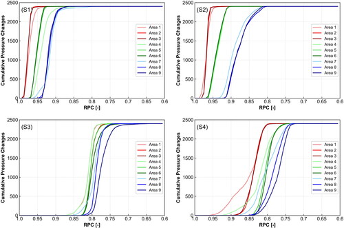
Figure 15. Sum lines of particle velocities perpendicular to the wall before recorded collisions. Cases S1 and S2 (top figures) are overshot situations, and Cases S3 and S4 (bottom figures) are undershot situations. The discharge increases from 50 m3/s (S1) to 110 m3/s (S2 and S3), and 240 m3/s (S4).
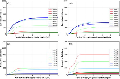
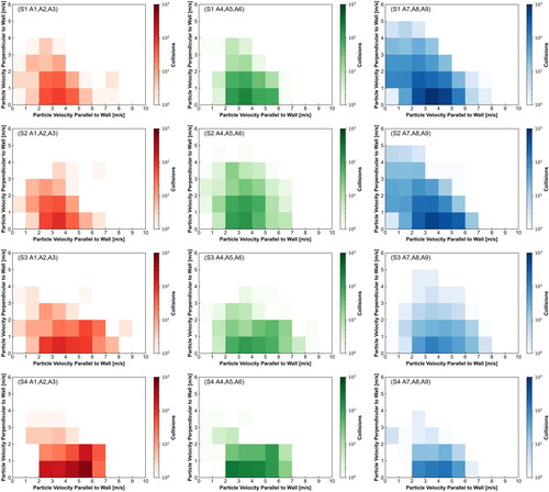
Figure 16. Number of recorded collisions divided according to the particle velocity perpendicular and parallel to the wall before the collision. Cases S1 and S2 (upper figures) are overshot situations, and cases S3 and S4 (lower figures) are undershot situations. The first column (red) is the upper starting areas A1–A3, the second column (green) the Middle starting areas A4–A6, and the third column (blue) is the lower starting areas A7–A9.