An empirical model of the decision to switch between electricity price contracts

Figures & data

Figure 9. Average survival function, price information only, homoscedastic specification.

The figure shows the average (over 250 possible histories of the variable price) survival function (survival with a variable-price contract) for different fixed prices based on the model specification which includes price information only and allows for information discounting.

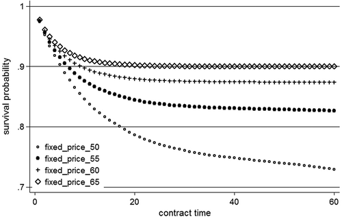
Figure 1. Number of Swedish households on each type of contract and price per kWh.

One SEK is roughly 0.1 Euro. Fixed-price contract refers to contracts with prices fixed for a year or longer (typically up to three years), and variable-price contract refers to contracts with prices varying by month. See footnote 1 for other type of contracts available to Swedish households. In addition to the price per kWh, households pay for transmission, green certificate and taxes. These costs (which are not included in the figure above) amounts to roughly 0.5 SEK/kWh, plus a fixed annual transmission fee varying between 1500 and 15000 SEK depending on the required amperage. These additional costs are identical for both type of contracts. The two vertical lines at June 2010 and February 2012 represents the time period during which households in the sample start their variable-price contract, as explained in Section 3. The households in the sample are then followed over time until June 2014.

Figure 2. Sign of log-likelihood ratio, Equation (13).

The two figures show how the sign of the log-likelihood ratio, given in (13), can vary across regions of the $(x_{t-1},x_t)$ plane for distinct values of the parameters. The shaded area in each case indicates the region in the plane where the log-likelihood ratio is positive, i.e. $(x_{t-1},x_t)$ increases the posterior odds in favour of $S=1$. The parameters for the regions on the left hand pane are: ${\mu }_{-}=-0.1,{\mu }_{+}=0.1,{\rho }_{-}=0.6,{\rho }_{+}=0.3,{\sigma }_{-}=0.65$ and ${\sigma }_{+}=0.55$. To produce the right hand pane, the parameters are identical except for ${\sigma }_{-}=0.55$ and ${\sigma }_{+}=0.65$.

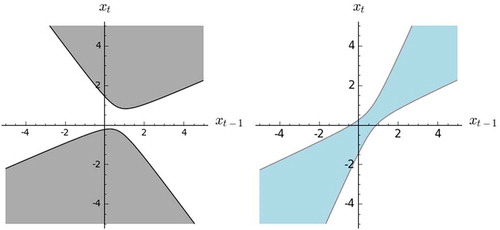
Figure 3. Log-odds, $ln{o}_2$ for $x_0=0$, $x_1=-1$, Equation (8).

Assuming that the first two realisations are $x_0=0$ and $x_1=-1$, the figure shows how the log-odds $ln{o}_2$, changes with $x_2$. The other parameters to define the two curves are: ${\mu }_{-}=-0.1,{\mu }_{+}=0.1,{\rho }_{-}=0.6$, and ${\rho }_{+}=0.3$.

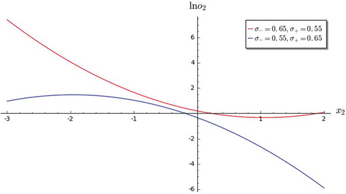
Table 1. Summary statistics.

	Mean	Standard deviation	Min	Max
Variable price, öre/kWh	43.35	11.21	0.21	0.927
Fixed price, öre/kWh	49.46	0.72	0.38	0.65
Temperature (Celsius)	4.58	8.18	−15.6	20.8
Monthly kWh, electrically heated villas	1473.13	1020.00	23	9515
Monthly kWh, non-electrically heated villa	964.92	869.40	2	9120
Monthly kWh, flats	735.01	843.33	1	6768
Income (1000’s SEK)	273.52	55.85	165	467
Age	49.07	4.55	35.4	66.9
Flats, share	0.79
Non-electrically heated villas, share	0.12
Electrically heated villas, share	0.09
Family size, share (more than two persons $=1$	0.34
University, share (University degree = 1)	0.22
Number of Households in sample	3353
Average Number of Months in sample	18

Note: Prices are excluding transmission, green certificate and taxes, which are independent of contract choice.

Figure 4. Seasonally adjusted temperature for Stockholm and Umeå.

The figure shows seasonally adjusted temperature (in degrees celsius, from month average) for Stockholm, located in the centre of Sweden and Umeå, located in the north of Sweden.

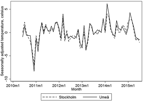
Figure 5. Seasonally adjusted log price differential and number of switches per month.

”Switches to fixed-price contract” refers to switches within the same supplier to a fixed-price contract, ”Switches to unknown” refers to switches to another retailer, and ”Entries” refers to number of new variable-price contracts per month. Our sample only includes households starting a variable-price contract between June 2010 and February 2012, so number of entries in the sample are zero after February 2012. ”Price differential” is the seasonally adjusted log price differential between the variable price and the fixed price..

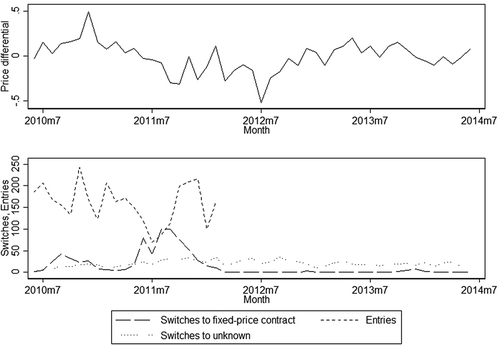
Table 2. Estimation summary.

Specification	(1)	(2)	(3)	(4)	(5)	(6)	(7)	(8)	(9)
No. of param.	2	2	2	3	3	3	14	14	14
Init. cond.	Yes	Yes	Yes	Yes	Yes	Yes	Yes	Yes	Yes
Trend		0.126 ***	0.152 ***		0.0708 ***	0.107 ***		−0.331 ***	−0.467 ***
		(0.007)	(0.013)		(0.008)	(0.013)		(0.040)	(0.051)
Discount			0.980 ***			0.978 ***			0.894 ***
			(0.007)			(0.005)			(0.015)
Number obs.	83786	83786	83786	83786	83786	83786	83786	83786	83786
Log-Likelihood	−3857.7	−3624.4	−3620.3	−3595.5	−3548.9	−3538.9	−3398.8	−3360.1	−3323.9
AIC	7765.3	7300.7	7294.7	7243.0	7151.8	7133.9	6867.6	6796.2	6725.8
BIC	7998.7	7543.4	7546.8	7485.7	7403.9	7395.3	7213.0	7151.0	7089.9

i) The table report maximum likelihood estimates based on the maximisation of expression (22) on the information in the sample. All specification accounts for the same initial characteristics. The number of parameters in the model of the log-likelihood ratio is reported in the second row.

ii) Columns 1–3 report on the estimation results for the univariate homoskedastic model of the log-likelihood ratio (described in Equation (A3)) where the information is the log price differential only. Column 4–6 report results for the univariate homoskedastic model (described in Equation (A3) in the Appendix A.2) where the mean log-price differential at time t depends on the local temperature deviation from monthly means. Column 7–9 report results for the bivariate heteroskedastic model where the information is both the log price differential and the temperature deviations from monthly averages. We report separately the estimates of the trend and discount parameters and their standard errors (in parentheses).

iii) The number of observations refer to the number of individuals $\times$ months observed in the sample.

iv) The log-likelihood statistics, Akaike’s and Schwarz’s Bayesian information criteria statistics are reported for each model. While a larger log-likelihood suggests a better fit, a smaller value of either information criteria suggests a better model. The information criteria penalise the fit with the number of parameter used.

Figure 6. Kaplan-Meier survival estimate.

The figure shows the Kaplan-Meier estimator for the proportion of households remaining on variable-price contracts over time.

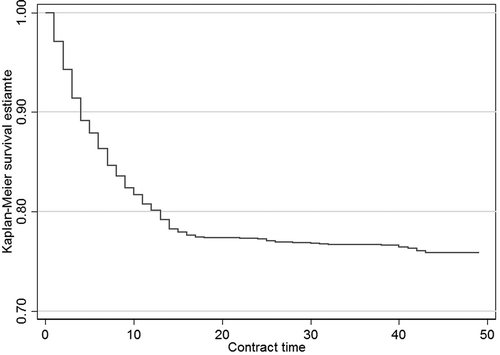
Figure 7. Average survival vs. history specific survival function.

The figure shows the average (over 250 possible histories of the variable price, continuous line) survival function (survival with a variable-price contract) at price $50$ öre/kWh against the survival function for 15 distinct variable price histories (dotted lines) based on the model specification which includes price information only and allows for information discounting.

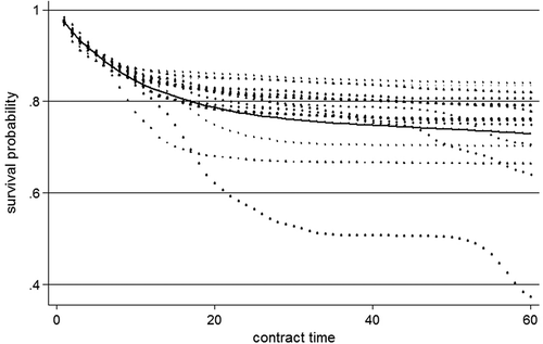
Figure 8. Average survival function, price and temperature information, heteroscedastic information.

The figure shows the average (over 250 possible histories of the variable price) survival function (survival with a variable-price contract) for different fixed prices based on the model specification which includes price and temperature information and allows for information discounting.

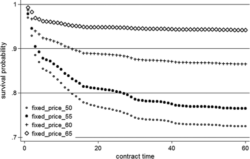
Figure A1. Sign of log-likelihood ratio, Equation (A3).

The two figures show how the sign of the log-likelihood ratio, given in Equation (A3), varies across regions of the $(x_{t-1},x_t)$ plane. The dotted and the dashed lines are the limits of the regions. In both figures, on the left (resp. right) of the dotted line the elasticity ${\eta }_{\lambda |x_t}$ is negative for all values of $x_t$ if $\mathrm{\Delta }\rho >0$ (resp. $\mathrm{\Delta }\rho <0$).

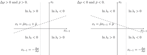
Table A1. Parameter estimates for specifications with univariate homoskedastic information (spec 1, 2 and 3) and bivariate homoskedastic information (spec 3, 4 and 5). 1.

	(1)	(2)	(3)	(4)	(5)	(6)
$x_{2,t}$	0.123	1.045 ***	1.297 ***	−1.406 ***	−0.407	−0.178
	(0.169)	(0.177)	(0.208)	(0.188)	(0.215)	(0.239)
$x_{2,t-1}$	−0.960 ***	−1.566 ***	−1.864 ***	−0.670 ***	−1.133 ***	−1.546 ***
	(0.169)	(0.176)	(0.213)	(0.171)	(0.181)	(0.216)
$x_{1,t}$				−0.153 ***	−0.106 ***	−0.118 ***
				(0.008)	(0.009)	(0.010)
Constant	4.719 ***	3.622 ***	3.690 ***	4.367 ***	3.854 ***	3.819 ***
	(0.371)	(0.373)	(0.373)	(0.374)	(0.376)	(0.376)
Trend		0.126 ***	0.152 ***		0.0708 ***	0.107 ***
		(0.007)	(0.013)		(0.008)	(0.013)
Discount			0.980 **			0.978 ***
			(0.007)			(0.005)
Number obs.	83786	83786	83786	83786	83786	83786
Log-likelihood	−3857.7	−3624.4	−3620.3	−3595.5	−3548.9	−3538.9
AIC	7765.3	7300.7	7294.7	7243.0	7151.8	7133.9
BIC	7998.7	7543.4	7546.8	7485.7	7403.9	7395.3

Standard errors in parentheses

* $p<0.05$, ** $p<0.01$, *** $p<0.001$

The table presents the parameters estimates for the transition model described in the main section of the paper assuming that the information is homoskedastic. $x_{1t}$ refers to the local temperature information (measured in deviations from local seasonal averages), and $x_{2t}$ refers to the price differential information (measured in deviations from seasonal averages). Specifications 1,2 and 3 present estimates assuming that the only relevant information is contained in the relative price differential. Specifications 4,5 and 6 add temperature to the relevant information.

Table A2. Parameter estimates for specifications with heteroskedasticity.

	(7)	(8)	(9)
$x_{2,t}^2$	0.609	10.55 ***	19.29 ***
	(1.705)	(2.404)	(3.632)
$x_{2,t}{x}_{1,t}$	−0.234	0.334	1.057 **
	(0.190)	(0.218)	(0.343)
$x_{2,t}{x}_{1,t-1}$	−0.580 **	−0.676 ***	0.010
	(0.192)	(0.197)	(0.258)
$x_{2,t}{x}_{2,t-1}$	−12.76 ***	−18.13 ***	−21.02 ***
	(2.673)	(2.910)	(3.507)
$x_{2,t}$	0.684 *	0.351	1.512 ***
	(0.304)	(0.321)	(0.414)
$x_{2,t-1}^2$	4.010 **	9.945 ***	14.90 ***
	(1.542)	(1.827)	(2.332)
$x_{2,t-1}$	−2.331 ***	−0.327	−0.944 *
	(0.296)	(0.386)	(0.455)
$x_{1,t}^2$	0.016 *	0.029 ***	0.065 ***
	(0.007)	(0.007)	(0.012)
$x_{1,t}{x}_{1,t-1}$	−0.053 ***	−0.065 ***	−0.049 **
	(0.011)	(0.01)	(0.015)
$x_{1,t}{x}_{2,t-1}$	0.488 ***	0.329 **	1.059 ***
	(0.122)	(0.125)	(0.189)
$x_{1,t}$	−0.076 ***	−0.055 *	−0.094 ***
	(0.021)	(0.022)	(0.027)
$x_{1,t-1}^2$	−0.014	0.002	0.0379 **
	(0.008)	(0.008)	(0.012)
$x_{1,t-1}{x}_{2,t-1}$	−0.809 ***	−0.294	−0.093
	(0.171)	(0.197)	(0.265)
$x_{1,t-1}$	0.021	0.092 ***	0.174 ***
	(0.022)	(0.024)	(0.032)
Constant	3.755 ***	3.899 ***	3.296 ***
	(0.378)	(0.378)	(0.382)
Trend		−0.331 ***	−0.467 ***
		(0.040)	(0.051)
Discount			0.894 ***
			(0.015)
Number obs.	83786	83786	83786
Log-likelihood	−3396.8	−3360.1	−3323.9
AIC	6867.6	6796.2	6725.8
BIC	7213.0	7151.0	7089.9

Standard errors in parentheses

*$p<0.05$, ** $p<0.01$, *** $p<0.001$

The table presents the parameters estimates for the transition model described in the main section of the paper assuming that the information is heteroskedastic. $x_{1t}$ refers to the local temperature information (measured in deviations from local seasonal averages), and $x_{2t}$ refers to the price differential information (measured in deviations from seasonal averages).

Table A3. Autoregressive models, ($ln$) variable price.

	Price only	Price and temperature
Constant	0.060	0.044
	(0.095)	(0.079)
$ln$ Variable price ($t-1$)	0.786 ***	0.769 ***
	(0.089)	(0.096)
Temperature ($t$)	–	−0.030 ***
		(0.007)
Temperature ($t-1$)	–	−0.018 ***
		(0.007)
$\sigma$	0.156 ***	0.136 ***
	(0.013)	(0.011)
Log-likelihood	26.37	34.79
Q-test stat	4.36	4.95
p-value (10 d-o-f)	0.93	0.90

Standard errors in parentheses

* $p<0.05$, ** $p<0.01$, *** $p<0.001$

i) The table report maximum likelihood estimates of the AR(1) models used to construct the alternative histories of the variable price. The models are estimated over the sample period of interest from June 2009 to June 2014 (61 observations).

ii) The Q-test statistics tests the null hypothesis that the residuals is the realisation of a white noise process. We test the first 10 autocorrelations.