
Figures & data
Scheme 1. Synthesis protocol for α-MnO2/PANI nanocomposite preparation.
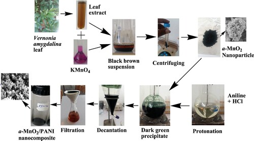
Table 1. Composition of α-MnO2 composite.
Figure 1. UV-Vis absorption spectra of α-MnO2 (a, black curve); PANI (b, red curve); and α-MnO2/PANI (c, blue curve).
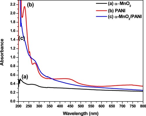
Figure 2. XRD patterns of (a) α-MnO2 nanosphere flower, (b) PANI powders, and (c) α-MnO2/PANI/ nanocomposite.
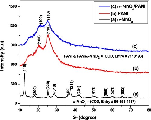
Table 2. XRD data used for calculation interlayer spacing, crystalline size of different sample.
Figure 3. FTIR spectra of (a) α-MnO2 (blue line), (b) PANI (black line), and (c) α-MnO2/PANI (red line) in the range from 4000 to 400 cm−1 with KBr pellet sampling.
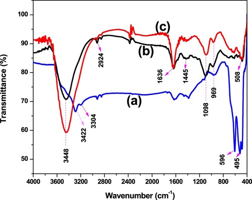
Figure 4. Thermogravimetric analysis (TGA, curve (a)) and differential thermal analysis (DTA, curve (b)) of α-MnO2 (blue line), PANI (black line), and α-MnO2/PANI (red line) NMs with flow rate 50 mL min−1 under N2 atmosphere.
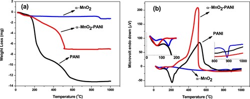
Figure 5. DSC thermogram of α-MnO2 (a), PANI (b), and α-MnO2/PANI (c) in N2 atmosphere (heating rate: 10°C min−1, flow rate: 20 mL min−1).
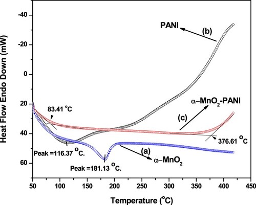
Figure 6. SEM images of (a) α-MnO2 NPs, (b) PANI, (c) α-MnO2/PANI composite, and (d) EDX spectrum of α-MnO2/PANI composite.
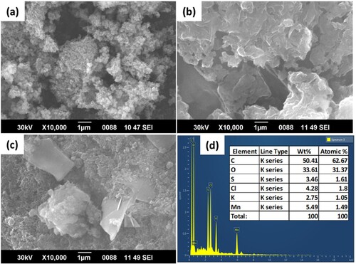
Figure 7. 2-D and 3-D SEM images of (a1) and (a2) from catalyst α-MnO2; (b1) and (b2) from catalyst PANI; (c1) and (c2) from catalyst α-MnO2/PANI.
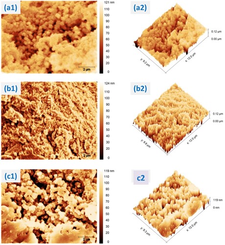
Figure 8. Dependence of mean pore size and surface area to volume ratio vs. number of pores for α-MnO2, PANI, and α-MnO2/PANI catalysts by the Watershed method.
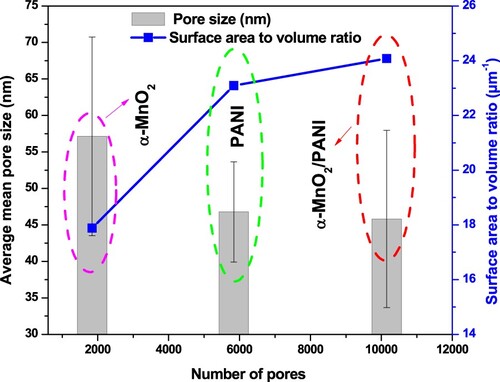
Table 3. Surface roughness statistical quantity results for different samples acquired from SEM entire image analysis.
Table 4. Pore size distribution comparison between this work and other literature.
Figure 9. Cyclic voltammogram (a) and the total charge exchanged from the beginning of the experiment, Q–Qo (b) of different catalyst modified electrodes. (i) bare PGE; (ii) α-MnO2/PGE; (iii) PANI/PGE; (iv) α-MnO2/PANI/PGE in 100 mM PBS (pH = 7.4) at a scan rate of50 mV s−1.
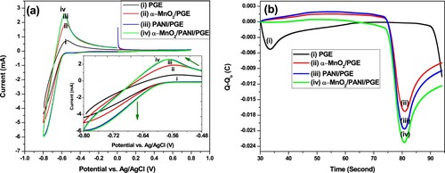
Figure 10. Cyclic voltammograms of α-MnO2/PANI/PGE electrode recorded at scan rates of 5–200 mVs−1 (inner to outer) (a), plot of peak currents vs. scan rates (b), variation of peak currents vs. square root of scan rate (c), and variation of log v vs. log Ipa (d) in 100 mM PBS (pH = 7.4).
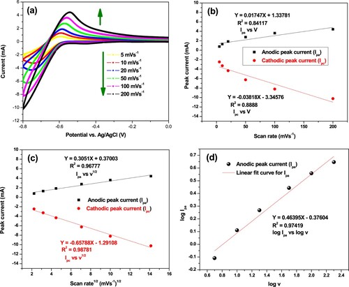
Figure 11. EIS plots Nyquist (a) and the inset displayed the equivalent circuit (Randles model with R.E is reference electrode and W.E is working electrode), Bode-magnitude (b), Bode-phase (c), and Admittance (d) plots of bare PGE, α-MnO2/PGE, PANI/PGE, and α-MnO2/PANI/PGE electrodes performed in 100 mM PBS (pH = 7.4).
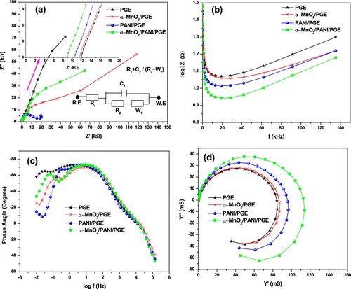
Table 5. Electrochemical parameters of the bare PGE, α-MnO2/PGE, PANI/PGE, and α-MnO2/PANI/PGE electrodes in 100 mM PBS (pH = 7.4) supporting electrolyte.
Figure 12. Plots of current vs. frequency (a) and Phase angle vs. current (b) for PGE (i), PANI/PGE (ii), α-MnO2/PGE (iii), and α-MnO2/PANI/PGE (iv).
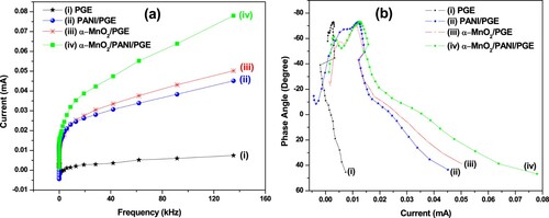
Figure 13. Variation of open circuit voltage (a) and variation of average open circuit voltage (b) with time.
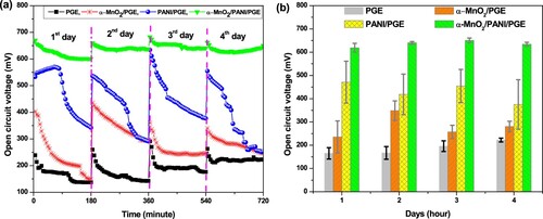
Figure 14. Polarization (a) and power density (b) curves.
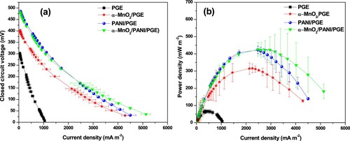
Figure 15. Dependence of power density with time (a) and external resistance (b), and profile of current discharge with time at different external resistance (c).
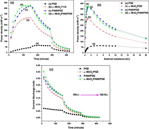
Table 6. Summary of optimum power density, operating voltage, stabilized time and resistance.
Table 7. Comparison of unmodified PGE, α-MnO2, PANI, and α-MnO2/PANI/PGE anode-based MFC with other literatures
Figure 16. Concentration removal (a) and their efficiency removal (b) for different anodic electrodes under open and closed circuit conditions.
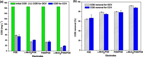
Figure 17. COD removal and coulombic efficiency for all anodic electrodes under glucose substrate during closed circuitconditions.
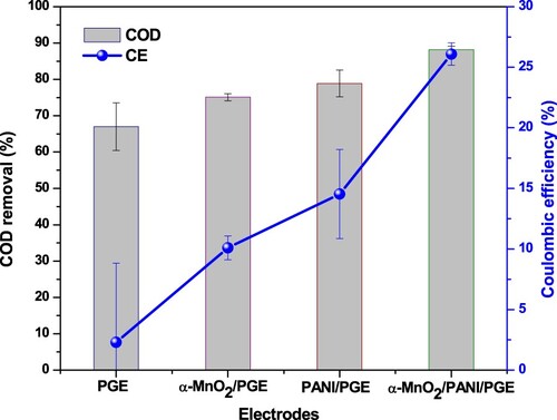
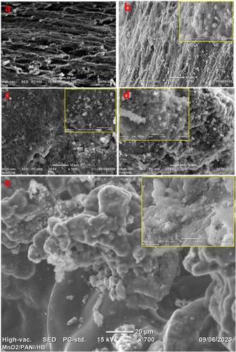
Figure 18. SEM images of (a) bare PGE and the attachment of E. coli cells on (b) PGE, (c) α-MnO2/ PGE, (d) PANI/PGE, and (e) α-MnO2/PANI/PGE anodes.
Supplemental Material
Download MS Word (2.3 MB)Data availability statement
The data that support the findings of this study are available in https://doi.org/10.6084/m9.figshare.13295507.v1