Experimental exploration of ErB₂ and SHAP analysis on a machine-learned model of magnetocaloric materials for materials design

Figures & data

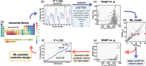
Figure 1. XRD pattern of ErB₂ (top) and LuB₂ (bottom) samples. Asterisks in the figure denote Er₂O₃ or Lu₂O₃ impurity. Dots correspond to the experimental data, while lines correspond to the calculated pattern by Rietveld analysis. Inset: Crystal structure of REB₂, drawn by VESTA software [16].

Figure 2. (a) Temperature dependence of magnetic susceptibility in ErB₂ (top) and its temperature-derivative (bottom), taken at $\mu$${ }_0$$H$ = 0.01 T. Inset shows isothermal magnetization curve of ErB₂, taken at $T$ = 5 K. (b) Inverse magnetic susceptibility of ErB₂ at 1 T. The dashed line in the figure is the fit to Curie–Weiss law in the temperature range of 200–300 K.

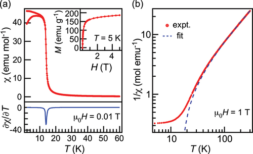
Figure 3. (a) Specific heat of ErB₂ under various magnetic fields. (b) Entropy curves of ErB₂ under magnetic fields deduced from data in (a). (c) $|\mathrm{\Delta }{S}_M|$ of ErB₂, obtained from data in (b). Gray open squares denote $|\mathrm{\Delta }{S}_M|$ estimated from magnetization curves (supplemental information S1). (d) $\mathrm{\Delta }{T}_{ad}$ of ErB₂, obtained from data in (b).

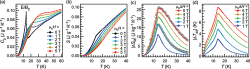
Figure 4. (a) Specific heat of ErB₂ and LuB₂ (left axis, solid lines) and estimated ${\mathrm{C}}_{mag}/T$ (right axis, dashed line). (b) Magnetic entropy curve of ErB₂ as a function of temperature.

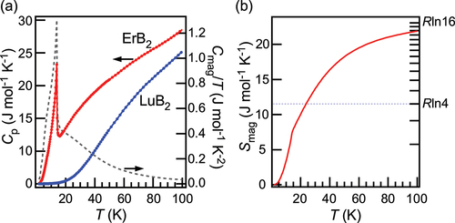
Figure 5. (a) Comparison of $|\mathrm{\Delta }{S}_M{|}^{peak}$ values in REB₂ (RE = Tb, Dy, Ho, Er, Tm) at ${\mu }_0\mathrm{\Delta }H$ = 5 T between experiment (left axis, black filled circles [4,10–12], and this work) and prediction by the machine-learned model (right axis, red open squares). (b) $|\mathrm{\Delta }{S}_M{|}^{peak}$ values predicted by machine-learned model plotted against the experimental values for REB₂ (red open squares) and those in the test dataset for the model (gray circles) [4].

Figure 6. Summary plots of SHAP values up to the top 15 compositional descriptors, sorted by (a) magnitude of the absolute mean (i.e. significance), and (b) magnitude of RE-dependence in REB₂ prediction. Dots in the figure represents each data point of the training dataset.

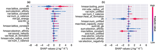
Figure 7. Top panel: Target values in training data (gray circles) plotted against focused compositional descriptors of (a) harmonic mean of boiling point, (b) minimum of van der Waals radius, and (c) maximum of molar heat capacity. Horizontal dashed lines correspond to the mean target value of training data (7.48). Predicted values for REB₂ are also shown as colored open squares. Middle panel: The same for SHAP values for corresponding compositional descriptors. Bottom panel: RE-dependence of SHAP values for corresponding compositional descriptors in the prediction for REB₂.

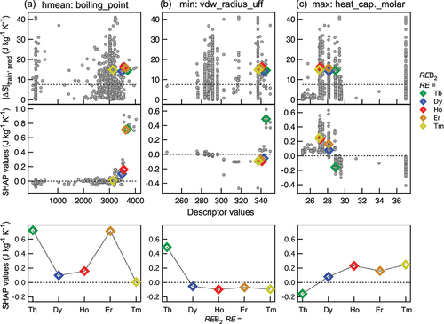
Figure 8. RE-dependence of SHAP values. (a) Total sum of SHAP values that is identical to predicted target values. (b) Partial sum of SHAP values. (c) Sum of SHAP values for the rest of descriptors.

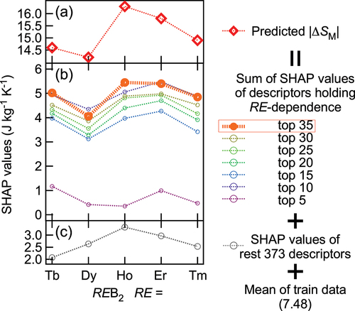
Figure 9. Schematic workflow of materials search using compositional descriptor-based machine-learning model (blue arrows) and proposed possible materials design assisted by SHAP analysis of the model. (a)(b) Focused physical property $f(X)$ for atomic elements (X). (c) Target plotted against compositional descriptor $g(\{f(X)\})$. (d) Constructed model by regression of data in (c). (e) SHAP value plotted against compositional descriptor $g$. (f) Sorted physical property for atomic elements (X).

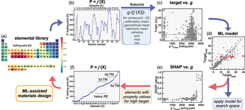
Figure 10. Left panel: Training data distribution of target plotted against focused compositional descriptors. Middle panel: The same as the left panel for SHAP values. Right panel: Heatmap of properties of atomic elements stored in XenonPy [6]. Focused compositional descriptors are the ones that exhibited the top five largest absolute mean SHAP values in the model (shown in Figure 6(a)), namely (a) maximum of lattice constant, (b) sum of electron affinity, (c) variance of lattice constant, (d) variance of the number of valence $p$-electrons, and (e) minimum of ground state energy in first principles software VASP [19]. Datapoints for several representative magnetocaloric materials are indicated explicitly, Gd₅Si_1.5Ge_2.5 [20], EuTiO₃ [21], EuS [22], ErCo₂ [23], La_0.8Ce_0.2Fe_11.7Si_1.3 [24] and abbreviated as GSG, ETO, ES, EC, LFS, respectively.

Momma K, Izumi F. VESTA: a three-dimensional visualization system for electronic and structural analysis. J Appl Crystallogr. 2008;41:653–658.

 Web of Science ®Google Scholar

de Castro PB, Terashima K, Yamamoto TD, et al. Machine-learning-guided discovery of the gigantic magnetocaloric effect in HoB2 near the hydrogen liquefaction temperature. NPG Asia Mater. 2020;12:35.

 Web of Science ®Google Scholar

Yamada H, Liu C, Wu S, et al. Predicting materials properties with little data using shotgun transfer learning. ACS Cent Sci. 2019;5:1717–1730.

 PubMed Web of Science ®Google Scholar

Kresse G, Hafner J. Ab initio molecular dynamics for liquid metals. Phys Rev B. 1993;47:558–561.

 PubMed Web of Science ®Google Scholar

Pecharsky A, Gschneidner K, Pecharsky V. The giant magnetocaloric effect between 190 and 300 K in the Gd5SixGe4–x alloys for 1.4≤x≤2.2. J Magn Magn Mater. 2003;267:60–68.

 Web of Science ®Google Scholar

Mo ZJ, Shen J, Li L, et al. Observation of giant magnetocaloric effect in EuTiO3. Mater Lett. 2015;158:282–284.

 Web of Science ®Google Scholar

Li D, Yamamura T, Nimori S, et al. Large reversible magnetocaloric effect in ferromagnetic semiconductor EuS. Solid State Commun. 2014;193:6–10.

 Web of Science ®Google Scholar

Wada H, Tomekawa S, Shiga M. Magnetocaloric properties of a first-order magnetic transition system ErCo2. Cryogenics. 1999;39:915–919.

 Web of Science ®Google Scholar

Chen X, Chen Y, Tang Y. The effect of different temperature annealing on phase relation of LaFe11.5Si1.5 and the magnetocaloric effects of La0.8Ce0.2Fe11.5–xCoxSi1.5 alloys. J Magn Magn Mater. 2011;323:3177–3183.

 Web of Science ®Google Scholar