Algorithms based on a 3-derivative method for singular differential equations including equations with blow-up solutions

Figures & data

Table 1. Coefficients of (5)

j	${\beta }_j$	$\beta {{ }^{\mathrm{\prime }}}_j$	${\gamma }_j$	$\gamma {{ }^{\mathrm{\prime }}}_j$	$p$	$C_{p+2}$	${\bar{C}}_{p+2}$
0	7/20	1/2	1/20	1/12	4	1/1440
1	3/20	1/2	−1/30	−1/12	4		1/720

Table 2. Coefficients for the predictors

j	${\bar{\beta }}_j$	${\overline{\beta { }^{\mathrm{\prime }}}}_j$	${\bar{\gamma }}_j$	${\overline{\gamma { }^{\mathrm{\prime }}}}_j$	${\delta }_j$	$\delta {{ }^{\mathrm{\prime }}}_j$	${\eta }_j$	$\eta {{ }^{\mathrm{\prime }}}_j$	$p$	$C{{ }^{\mathrm{\prime }}}_{p+2}$	${\overline{C{ }^{\mathrm{\prime }}}}_{p+2}$
0	1/2	1	1/6	1/2	1/24	1/24	1/120	1/24	4	1/720	1/120

Table 3. Maximum errors for different step sizes for Example, 3.1

$N$	TDNM	ROC	Othmar (Koch et al., 2000)	ROC
5	$7.08\times {10}^{-5}$		$1.5\times {10}^{-2}$	3.993
10	$4.06\times {10}^{-6}$	4.126	$9.7\times {10}^{-3}$	5.105
20	$2.38\times {10}^{-7}$	4.091	$2.8\times {10}^{-5}$	5.058
40	$1.45\times {10}^{-8}$	4.034	$8.5\times {10}^{-6}$	5.024
80	$9.01\times {10}^{-10}$	4.011	$2.6\times {10}^{-8}$	5.012
160	$5.62\times {10}^{-11}$	4.003	$8.1\times {10}^{-9}$	5.007

Table 4. Errors for the variable step implementation of the TDNM for Example, 3.1

$Tol$	$[0,1]$ Error	Nmax	$[0,10]$ Error	Nmax
${10}^{-4}$	$4.28\times {10}^{-5}$	8	$1.27\times {10}^{-3}$	51
${10}^{-6}$	$3.14\times {10}^{-6}$	16	$5.17\times {10}^{-4}$	101
${10}^{-8}$	$1.78\times {10}^{-7}$	26	$2.80\times {10}^{-6}$	204

Table 5. Maximum errors for different stepsizes for Example, 3.2

$N$	TDNM	ROC	Othmar (Koch et al., 2000)	ROC
5	$4.98\times {10}^{-7}$		$8.1\times {10}^{-3}$	4.954
10	$2.65\times {10}^{-8}$	4.235	$2.6\times {10}^{-5}$	5.079
20	$1.54\times {10}^{-9}$	4.103	$7.7\times {10}^{-6}$	5.095
40	$9.28\times {10}^{-11}$	4.052	$2.2\times {10}^{-8}$	5.084
80	$5.69\times {10}^{-12}$	4.028	$6.6\times {10}^{-9}$	4.995
160	$3.49\times {10}^{-13}$	4.026

Table 6. Errors for the variable step implementation of the TDNM for Example, 3.2

$Tol$	$[0,1]$Error	Nmax	$[0,10]$ Error	Nmax
${10}^{-4}$	$2.59\times {10}^{-4}$	12	$2.59\times {10}^{-4}$	21
${10}^{-6}$	$1.17\times {10}^{-6}$	15	$2.49\times {10}^{-6}$	32
${10}^{-8}$	$3.92\times {10}^{-8}$	21	$1.60\times {10}^{-7}$	57

Table 7. Maximum errors for different step sizes for Example, 3.3

$N$	TDNM	ROC	Method in (Weinmüller, 1986)
4	$1.743\times {10}^{-6}$		$5.079\times {10}^{-3}$
8	$1.221\times {10}^{-7}$	3.835	$1.219\times {10}^{-3}$
16	$8.286\times {10}^{-9}$	3.881	$3.018\times {10}^{-4}$
32	$5.339\times {10}^{-10}$	3.956	$7.526\times {10}^{-5}$
64	$3.389\times {10}^{-11}$	3.978	$1.880\times {10}^{-5}$
128	$2.136\times {10}^{-12}$	3.988	$4.700\times {10}^{-6}$

Table 8. Maximum errors for different stepsizes for Example, 3.4

$N$	TDNM	ROC	Method in (Rashidinia et al., 2007)	TDNM	ROC	Method in (Rashidinia et al., 2007)
		$r=0.25$			$r=0.75$
16	$3.69\times {10}^{-6}$		$2.47\times {10}^{-6}$	$2.33\times {10}^{-6}$		$1.27\times {10}^{-6}$
32	$2.29\times {10}^{-7}$	4.014	$2.04\times {10}^{-6}$	$1.43\times {10}^{-7}$	4.027	$1.15\times {10}^{-6}$
64	$1.43\times {10}^{-8}$	4.003	$3.09\times {10}^{-7}$	$8.91\times {10}^{-9}$	4.001	$1.56\times {10}^{-7}$
128	$8.90\times {10}^{-10}$	4.001	$3.06\times {10}^{-7}$	$5.56\times {10}^{-10}$	4.002	$1.16\times {10}^{-7}$
256	$5.56\times {10}^{-11}$	4.001	$3.03\times {10}^{-8}$	$3.47\times {10}^{-11}$	4.001	$1.65\times {10}^{-8}$
512	$3.46\times {10}^{-12}$	4.009	$3.00\times {10}^{-8}$	$2.15\times {10}^{-12}$	4.013	$1.17\times {10}^{-8}$

Table 9. Comparison of absolute errors $E_N(x)$ for Example, 3.5

		TDNM			Xie et al (Xie et al., 2016)
$x$	$E_{10}(x)$	$E_{20}(x)$	$E_{40}(x)$	$E_{10}(x)$	$E_{20}(x)$	$E_{40}(x)$
0.0	$1.87\times {10}^{-14}$	$7.88\times {10}^{-15}$	$3.83\times {10}^{-15}$	$1.05\times {10}^{-5}$	$2.2\times {10}^{-9}$	$1.4\times {10}^{-9}$
0.1	$8.38\times {10}^{-9}$	$8.54\times {10}^{-10}$	$6.84\times {10}^{-11}$	$1.05\times {10}^{-5}$	$1.2\times {10}^{-9}$	$4.0\times {10}^{-10}$
0.2	$1.42\times {10}^{-8}$	$1.13\times {10}^{-9}$	$8.16\times {10}^{-11}$	$1.03\times {10}^{-5}$	$1.4\times {10}^{-9}$	$6.0\times {10}^{-10}$
0.3	$1.51\times {10}^{-8}$	$1.14\times {10}^{-9}$	$7.94\times {10}^{-11}$	$1.02\times {10}^{-5}$	$1.4\times {10}^{-9}$	$6.0\times {10}^{-10}$
0.4	$1.36\times {10}^{-8}$	$9.98\times {10}^{-10}$	$6.90\times {10}^{-11}$	$9.93\times {10}^{-6}$	$1.5\times {10}^{-9}$	$8.0\times {10}^{-10}$
0.5	$1.08\times {10}^{-8}$	$7.85\times {10}^{-10}$	$5.42\times {10}^{-11}$	$9.62\times {10}^{-6}$	$2.6\times {10}^{-9}$	$1.8\times {10}^{-9}$
0.6	$7.39\times {10}^{-9}$	$5.46\times {10}^{-10}$	$3.80\times {10}^{-11}$	$9.25\times {10}^{-6}$	$1.9\times {10}^{-9}$	$1.2\times {10}^{-9}$
0.7	$4.17\times {10}^{-9}$	$3.20\times {10}^{-10}$	$2.27\times {10}^{-11}$	$8.75\times {10}^{-6}$	$1.4\times {10}^{-9}$	$7.0\times {10}^{-10}$
0.8	$1.64\times {10}^{-9}$	$1.40\times {10}^{-10}$	$1.04\times {10}^{-11}$	$7.88\times {10}^{-6}$	$9.0\times {10}^{-10}$	$3.0\times {10}^{-10}$
0.9	$1.66\times {10}^{-10}$	$2.79\times {10}^{-11}$	$2.55\times {10}^{-12}$	$5.78\times {10}^{-6}$	$5.5\times {10}^{-10}$	$1.1\times {10}^{-9}$
1.0	0.00	0.00	0.00	$1.10\times {10}^{-10}$	$2.74\times {10}^{-11}$	$3.6\times {10}^{-11}$

Figure 1. Graphical evidence for Example, 3.6, $M=20,N=80.$ The blow-up in the analytical solution given by (b) is in agreement with that of the approximate solution given by (a). As $t\to 1$, $x\to 1$, $u(1,1)\to \mathrm{\infty }$, which is in agreement with the approximate solution.

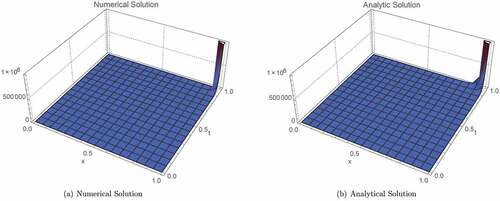
Figure 2. The results provided by the TDNM is in good agreement with the analytical solution. As $t\to 1$, both the analytical and the approximate solutions blow-up.

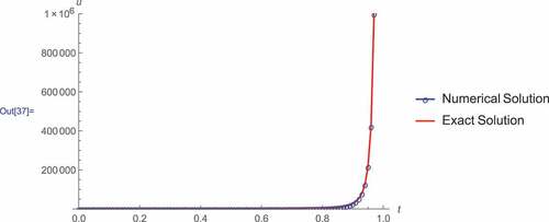
Figure 3. The results provided by the TDNM (M = 10, N = 40) in block unification mode is in good agreement with the analytical solution. We observe that at $x=1$, where a numerical method could perform poorly, the numerical solution is still in good agreement with the analytical solution.

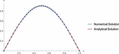
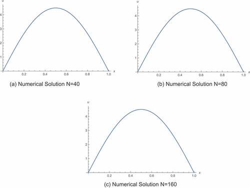
Figure 4. Graphical evidence for Example, 3.7, $M=10,N=40$. The results provided by the TDNM in block unification mode are in good agreement with the exact solution, and the errors are also small, validating the fact the TDNM performs well when applied to parabolic equations.

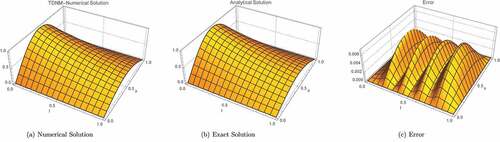
Figure 5. Graphical evidence for Example, 3.8. By considering the reference blow-up time of $T=8.24371\times {10}^{-2}$ for $M=10,N=40,N=80,N=160$, the blow-up time is located only at the point $x=0.5$.

Koch, O., Kofler, P., & Weinmüller, E. B. (2000). The implicit Euler method for the numerical solution of singular initial value problems. Applied Numerical Mathematics, 34(2–3), 231–252. https://doi.org/10.1016/S0168-9274(99)00130-0

 Web of Science ®Google Scholar

Weinmüller, E. B. (1986). On the numerical solution of singular boundary value problems of second order by a difference method. Mathematics of Computation, 46(173), 93–117. https://doi.org/10.1090/S0025-5718-1986-0815834-X

 Web of Science ®Google Scholar

Rashidinia, J., Mohammadi, R., & Jalilian, R. (2007). The numerical solution of non-linear singular boundary value problems arising in physiology. Applied Mathematics and Computation, 185(1), 360–367. https://doi.org/10.1016/j.amc.2006.06.104

 Web of Science ®Google Scholar

Xie, L., Zhou, C., & Xu, S. (2016). An effective numerical method to solve a class of nonlinear singular boundary value problems using improved differential transform method. SpringerPlus, 5(1), 1066. https://doi.org/10.1186/s40064-016-2753-9

 Google Scholar