
Figures & data
Table 1.
,
,
and
for Example, 5.1 using method (3.19) and scheme(3.19) with Richardson extrapolation (4.10) with
Table 2.
,
,
and
for Example, 5.2 using method (3.19) and scheme(3.19) with Richardson extrapolation (4.10) with
Table 3.
,
,
and
for Example, 5.3 using method (3.19) and method (3.19) with Richardson extrapolation (4.10) with
Table 4.
,
and
for Example, 5.1 using proposed method (3.19) with Richardson extrapolation (4.10) and results in (Mesfin M. Woldaregay & Duressa, Citation2019) and (Woldaregay & Duressa, Citation2020) with
Figure 1. The effect of on the solution profiles at
and
.
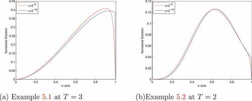
Figure 2. The effect of on the solution profiles at
.
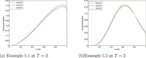
Figure 3. The effect of on the solution profiles with
.
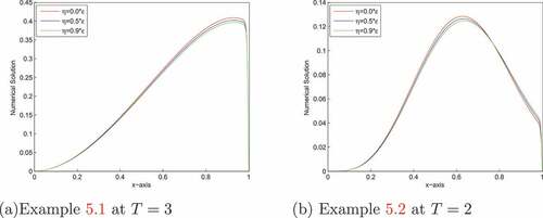
Figure 4. Numerical solution profiles for Example, 5.1 at .
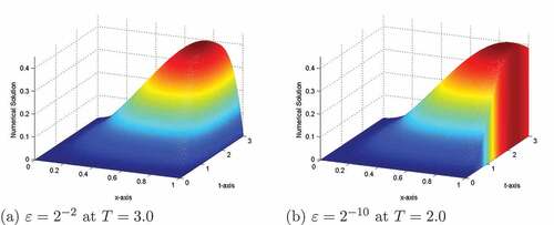
Figure 5. Numerical solution profiles for Example, (5.2) at and
.
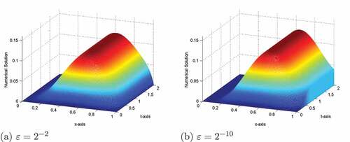
Figure 6. Numerical solution profiles for Example, 5.3 at and
.
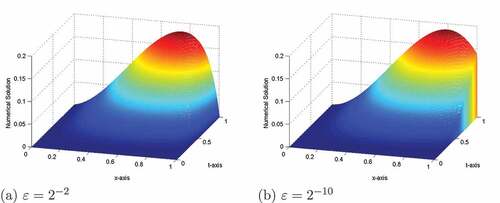
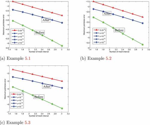
Figure 7. Log-log plot for the maximum absolute errors before and after the Richardson extrapolation technique.
Data availability statement
No data were used to support the study.