Uniform persistence and backward bifurcation of vertically transmitted vector-borne diseases

Figures & data

Table 1. Model parameter and their descriptions

Parameter	Description (rates are per day)
µ	natural mortality rate of hosts
ζ	vertical disease transmission rate from female mosquito to egg
δ0	average number of new adult female mosquitoes
δ1	a factor for density dependent maturation to adulthood
Λ	per capita birth rate of hosts
r	recovery rate of hosts
β	the probability of disease transmission from infectious vector to susceptible host
	from an infected vector to a susceptible host
ρ	immigration rate of susceptible hosts
ϕ	the number of bites a host sustains from a mosquito(host-vector contact rate)
α	disease-induced host death rate
ψ	fading rate of treatment to make hosts susceptible to the disease
γ	mortality rate of vectors
φ	incubation rate of the disease in a vector
d	incubation rate of the disease in a host
θ1	probability of disease transmission from infectious host to vector
θ2	probability of disease transmission from exposed host to vector

Figure 1. A time plot reflecting the effects of vertical transmission in the vector population on disease prevalence: ζ = 0.0046 (continuous/green curve), ζ = 0.3046 (dashed/blue curve) and ζ = 0.5046 (continuous/red curve). Other parameters are $\alpha =0.0065$, $\gamma =1/17$, $\beta =0.15,{\theta }_1=0.0083,{\theta }_2=0.0072$, $\mu =3.91\times {10}^{-5},\text{upLambda}=1.48\times {10}^{-5},\rho =205,{\delta }_0=1150,r=1/7,{\delta }_1=0.0397,d=1/6,\psi =0.00243,\varphi =2.$ For each case ${\mathcal{R}}_0<1$.

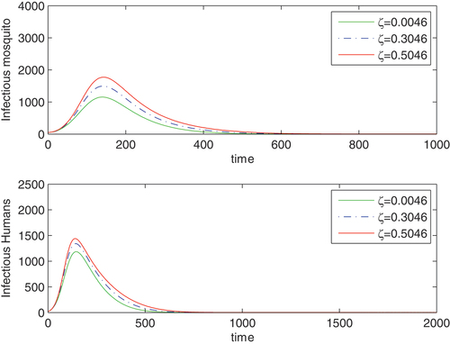
Figure 2. Bifurcation curves reflecting the results of theorem (4.3). Unstable branch (red), stable branch (blue), green (extinction); α = 0.0062 (continuous curve) and α = 0.0013 (dashed curve). Other parameters are $\gamma =1/17,$ β = 0.15, $\zeta =0.77,{\theta }_1=0.0083,{\theta }_2=0.0063$, $\mu =3.91\times {10}^{-5},\text{upLambda}=1.56\times {10}^{-5},\rho =200,{\delta }_0=1100,r=1/7,{\delta }_1=0.0399,d=1/6,\phi =1/8,\psi =0.00233,\varphi =2.$ based on the data we used in this figure, we have $\mathcal{F}=0.0015,$ for $\alpha =0.0062,$ $\frac{{\mathcal{H}}_1}{k_2}+2d\alpha =7.8937\times {10}^{-4}$ and $\frac{\rho k_3{k}_4}{y_1^{\ast }}\sqrt{\frac{({\theta }_{1}d+{\theta }_2{k}_3)k_1{y}_1^{\ast }}{\beta \phi k_3(\gamma k_4-{\delta }_1\zeta \phi )x_1^{\ast }}}=3.4734\times {10}^{-5}.$ for $\alpha =0.0013,$ $\frac{{\mathcal{H}}_1}{k_2}+2d\alpha =-2.7186\times {10}^{-5}$ and $\frac{\rho k_3{k}_4}{y_1^{\ast }}\sqrt{\frac{({\theta }_{1}d+{\theta }_2{k}_3)k_1{y}_1^{\ast }}{\beta \phi k_3(\gamma k_4-{\delta }_1\zeta \phi )x_1^{\ast }}}=3.3930\times {10}^{-5}.$ the bifurcation is backward for α = 0.0062 and forward when α = 0.0013.

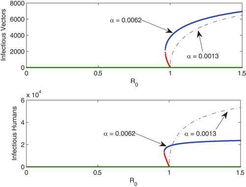
Figure 3. Endemic asymptotic level of infectious mosquitoes and humans for ${\mathcal{R}}_0<1.$ ζ = 0.77 $\alpha =0.038,$ $\gamma =1/18,$ $\beta =0.87,{\theta }_1=0.0079,{\theta }_2=0.0072,$ $\mu =3.91\times {10}^{-5},\text{upLambda}=1.48\times {10}^{-5},\rho =200,{\delta }_0=1120,r=1/7,{\delta }_1=0.0397,d=1/6,\psi =0.00233,\varphi =2,\phi =1/8.$ for these set of parameters, ${\mathcal{R}}_0=0.3944<1,$ but mosquito and human populations equilibrate to endemic levels (see time plots (a) and (c) with initial value $(20,40,1500,40,2000,40,10000)$). The bifurcation diagrams of mosquitoes and humans as ${\mathcal{R}}_0$ changes given in windows (b) and (d) show backward bifurcations where two endemic equilibria exists for ${\mathcal{R}}_0<1$.

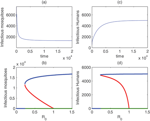
Table 2. Parameter estimation for dengue fever. Rate is per day

Par.	Range	Ref.	Par.	Range	Ref.
γ	$[1/17,1/10]$	(Centers for Disease Control and Prevention: Malaria)	δ0	$[700,10,000]$	estimate
µ	$[\frac{1}{70(356)},\frac{1}{45(356)}]$	(WHO)	θ1	$[0,1)$	estimate
ϕ	$\ge 1$	variable	α	$(0,0.1)$	Chitnis et al. (2013), (WHO)
φ	$[1/14,1/7]$	Chan et al. (2012)	ψ	$[0,1)$	estimate
r	$[0,1/7]$	Adams and Boots (2010)	β	$(0,1)$	estimate
ζ	$[0,1)$	estimate	δ1	$[0,\gamma )$	estimate
d	$[1/14,1/3]$	(Centers for Disease Control and Prevention)	ρ	$\ge 1$	variable
θ2	$[0,{\theta }_1)$	estimate
Λ	$(0,\mu )$	estimate

Centers for Disease Control and Prevention: Malaria. http://www.cdc.gov/Malaria/faq.htm2

 Google Scholar

WHO. https://who.int/news-room/fact-sheets/detail/dengue-and-sever-dengue.

 Google Scholar

Chitnis, N., Hyman, J. M., & Manore, C. A. (2013). Modelling vertical transmission in vector-borne diseases with application to Rift Valley fever. Journal of Biological Dynamics, 7(1), 11–40. https://doi.org/10.1080/17513758.2012.733427

 PubMed Web of Science ®Google Scholar

Chan, M., Johansson, M. A., & Vasilakis, N. (2012). The incubation periods of dengue viruses. PLoS ONE, 7(11), e50972. https://doi.org/10.1371/journal.pone.0050972

 PubMed Web of Science ®Google Scholar

Adams, B., & Boots, M. (2010). How important is vertical transmission in mosquitoes for the persistence of dengue? Insights from a mathematical model. Epidemics, 2(1), 1–10. https://doi.org/10.1016/j.epidem.2010.01.001

 PubMed Web of Science ®Google Scholar

Centers for Disease Control and Prevention. http://www.cdc.gov/dengue

 Google Scholar