Figures & data
FIGURE 1 Location of study sites (dots on left panel) in the Department Cajamarca (middle panel) in Peru, South America. The study area is centered at 6°54′S, 78°22′W.
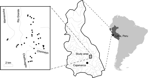
FIGURE 2 View of wetland Cocañes 3 looking southeast, illustrating its three major groundwater flow systems indicated by arrows. The water flowing from the near side of the wetland (two black arrows) has pH ranging from 6.4 to 6.7, while that from the far side (white arrow) is highly acid with pH ranging from 4.3 to 4.7. The two areas support different plant species and plant communities.
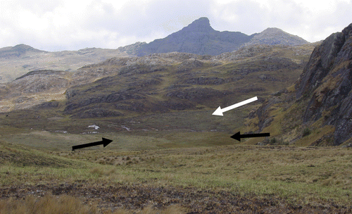
FIGURE 3 Number (N) of plots with groundwater pH in 0.5 unit categories.
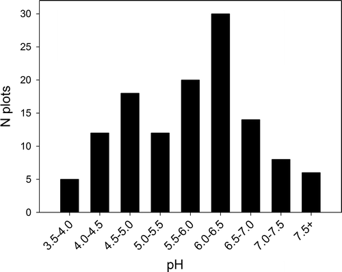
Table 1 Ion and metal concentrations, in mg L−1, for samples from the study wetlands listed by site. Ca = calcium, Mg = magnesium, Na = sodium, K = potassium, HCO3 = bicarbonate, Cl = chloride, Cu = copper, Fe = iron, SO4 = sulfate. Sum of cations, anions, and sum of ions are presented as well as the water type based upon the major cations and anions present. Cells that are left blank are below detection levels (0.5 mg L−1 for Cl, 0.005 mg L−1 for Cu, and 0.01 mg L−1 for Fe).
FIGURE 4 Piper plot showing proportion of Ca, Mg, and Na+K in bottom left ternary plot; SO4, HCO3, and Cl in the bottom right ternary plot; and the combined ion combinations in the top plot. Triangles are plots with pH < 5.0, x plots with pH 5.0–6.0, and circles plots with pH > 6.0.
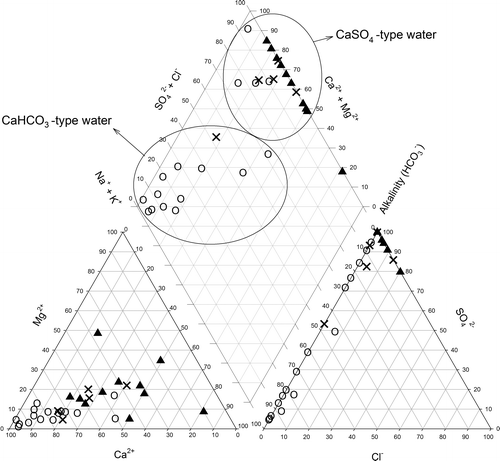
FIGURE 5 Number (N) of plots containing percent (%) soil organic carbon in seven categories.
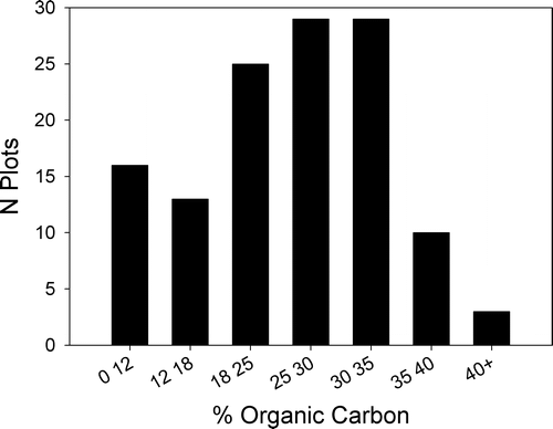
FIGURE 6 Number (N) of plots containing peat soil thickness in nine categories.
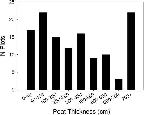
Table 2 Number of vascular plant taxa and proportion of flora by family.
FIGURE 7 Photographs of four of the major vegetation types. (A) Cushion plant community heavily damaged by livestock trampling showing the Plantago tubulosa–Oreobolus obtusangulus–Werneria pygmaea–Distichia acicularis community. (B) Sedge vegetation in plot showing the Carex pichinchensis–Scorpidium scorpioides–Cratoneuron filicinum community. (C) Bryophyte- and lichen-dominated vegetation showing the Sphagnum magellanicum–Cladina confusa–Loricaria lycopodinea community. The dark plant is Loricaria lycopodinea. (D) Tussock grass community showing the Cortaderia hapalotricha–Cortaderia sericantha community.
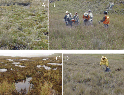
FIGURE 8 CCA analysis of all plots along axes 1 and 2, showing the vectors for statistically significant environmental variables. Eigenvalue of the first canonical axis is 0.507 and is statistically significant at P < 0.01 using a Monte Carlo permutation test. The sum of all canonical eigenvalues was also significant at P < 0.01, demonstrating that the relation between the species and the environmental variables is highly significant (P < 0.01). Numbers are plots assigned to each community type.
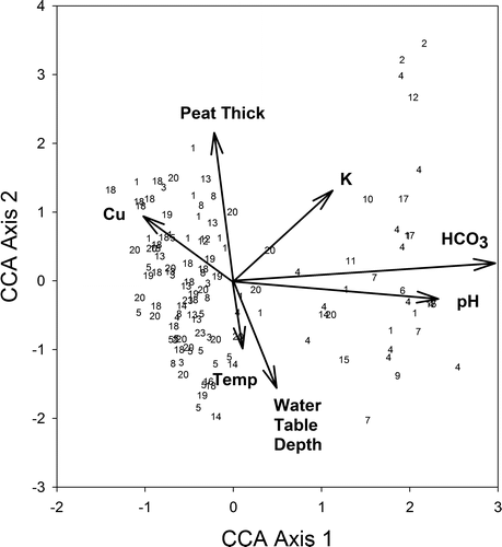
Table 3 Results of the canonical correspondence analysis showing eigenvalues for the first four axes, as well as the species environment correlations, and cumulative variance in species and species environment relation data and the total inertia in the data set. The lower portion of the table includes the canonical coefficients, and intraset correlation coefficients of environmental variables with the first two ordination axes are also shown. Axis variables are pH, WT (water table depth), peat thickness (Peat), % organic carbon (%OC), soil temperature at 13 and 28 cm depth (13 cm and 28 cm), wetland slope, aspect, and dissolved HCO3, total N, total P, Cl, SO4, Cu, Fe, Mg, K, and Na. Variables in bold explained a statistically significant proportion of the variance as determined using a Monte Carlo permutation test (499 runs) (P < 0.05).
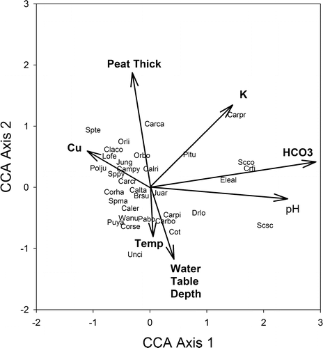
FIGURE 9 CCA analysis showing the centroids of diagnostic plant species along axes 1 and 2, showing the vectors for statistically significant environmental variables. Species shown in the ordination space are: Brsu = Breutelia subarcuata, Calta = Calamagrostis tarmensis, Capy = Campylopus spp., Carca = Carex camptoglochin, Carbo = Carex bonplandii, Carcr = Carex crinalis, Carpi = Carex pichinchensis, Claco = Cladina confusa, Corha = Cortaderia hapalotricha, Corse = Cortaderia sericantha, Cot = Cotula australis, Crfi = Cratoneuron filicinum, Drlo = Drepanocladus longifolius, Eleal = Eleocharis albibracteata, Juar = Juncus arcticus, Jung = Jungermannia sp., Lofe = Loricaria lycopodinea, Orbo = Oreobolus obtusangulus, Orli = Orithrophium limnophilum, Pabo = Paspalum bonplandianum, Pltu = Plantago tubulosa, Polju = Polytrichum juniperinum, Puya = Puya fastuosa, Scco = Scorpidium cossonii, Scsc = Scorpidium scorpioides, Spma = Sphagnum magellanicum, Spte = Sphagnum tenellum, Sppy = Sphagnum pylaesii, Sp1 = Sphagnum unknown species 1, Wanu = Werneria nubigena, Unci = Uncinia hamata.
Appendix A Vascular plant taxa found in study plots. N is the number of stands in which the taxon was recorded. Mean is the mean canopy cover in all plots, and SD is the standard deviation of mean canopy cover. Distribution is the known geographic distribution of the taxon.
Appendix B Bryophyte taxa identified in the study plots. N is the number of stands in which the taxon was recorded, mean is the mean percent canopy cover for study stands, and SD is the standard deviation of the mean of percent canopy cover.
Appendix C Lichen taxa in study plots. N is the number of stands in which the taxon was recorded, mean is the mean percent canopy cover for study stands, and SD is the standard deviation of the mean of percent canopy cover.