
Figures & data
Figure 1 Synthesis of flurbiprofen–antioxidant mutual prodrugs.
Abbreviation: DMF, dimethylformamide.
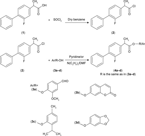
Figure 2 In vitro hydrolytic pattern of the ester prodrugs (4a–d) in SIF (pH 7.4).
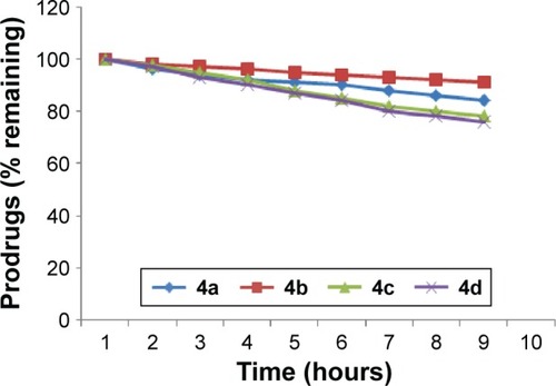
Figure 3 In vitro hydrolytic pattern of the ester prodrugs (4a–d) in 80% human plasma (pH 7.4).
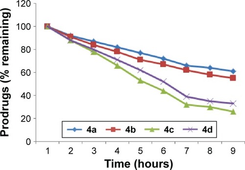
Table 1 Determination of anti-inflammatory activity of different derivatives of flurbiprofen by the carrageenan hind paw edema method
Table 2 Determination of anti-inflammatory activity of different derivatives of flurbiprofen by egg albumin-induced paw edema in mice
Table 3 Determination of the analgesic activity of derivatives of flurbiprofen by the acetic acid-induced writhing method in mice
Table 4 Determination of analgesic activity of selective flurbiprofen derivatives by the formalin-induced paw licking method in mice
Table 5 Effect of test compounds against brewer’s yeast-induced pyrexia in mice
Table 6 Ulcerogenic activity of synthesized prodrugs (4a–d) and flurbiprofen
Table 7 Chemoinformatics and molecular properties of ligand molecules
Table 8 COX-1 and COX-2 docking energy values
Figure 4 Binding interaction of COX-1 against five different inhibitors.
Abbreviation: COX-1, cyclooxygenase 1.
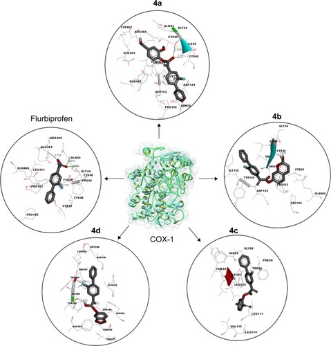
Figure 5 Binding interaction of COX-2 against five different inhibitors.
Abbreviation: COX-2, cyclooxygenase 2.
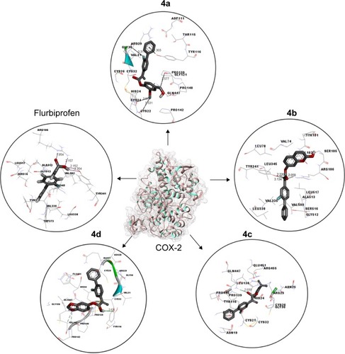
Figure 6 RMSD graph of COX-1 and COX-2 proteins at different time scales from 0 ps to 10,000 ps.
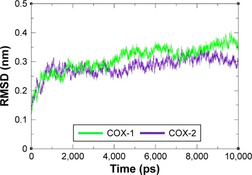
Figure 7 RMSF graph of COX-1 and COX-2 at different time scales from 0 ps to 10,000 ps.
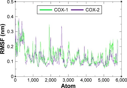
Figure 8 Rg graph of COX-1 and COX-2 at different time scales from 0 ps to 10,000 ps.
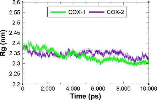
Figure 9 Solvent accessible surface area graph of COX-1 and COX-2 at different time scales from 0 ps to 10,000 ps.
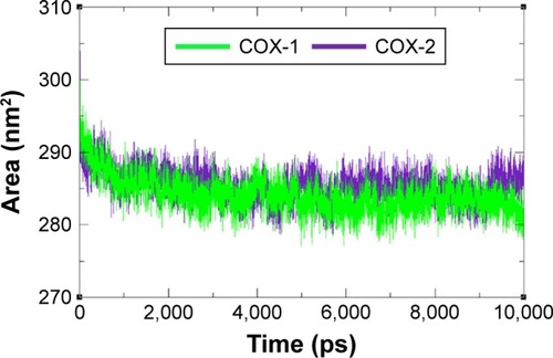
Figure S1 Superimposed structures of COX-1 and COX-2 with binding pocket.
Figure S2 The hydrophobic graphs for predicted model of COX-1, having row index (number of residues) at x-axis and hydrophobic value at y-axis.
Abbreviation: COX, cyclooxygenase.
Figure S3 The hydrophobic graphs for predicted model of COX-2, having row index (number of residues) at x-axis and hydrophobic value at y-axis.
Abbreviation: COX, cyclooxygenase.
Figure S4 Ramachandran plot of COX-1.
Abbreviation: COX, cyclooxygenase.
Figure S5 Ramachandran plot of COX-2.
Abbreviation: COX, cyclooxygenase.
Table S1 The clinical effects on animals during the experiments