Figures & data
Figure 1 Numerical simulation results of cylindrical magnetic susceptibility reconstructions. The 3D cylindrical volumes are displayed with three orthogonal central slices (x-slice, y-slice, and z-slice). (A) A predefined cylindrical susceptibility map (ground truth). (B) T2* phase image (calculated by T2*MRI simulation). Note that the main field B0 (marked in red arrow) is perpendicular to the cylinder axis; (C) χ reconstruction by filter truncation solver (‘trunc recon’) (Equation 5 with threshold ε0=0.12); (D) χ reconstruction by TV-regularized 3-subproblem Bregman iteration solver (‘TV3 recon’);Citation13 (E) χ reconstruction by TV-regularized 2-subproblem Bregman iteration solver (‘TV2 recon’) (Equation 12). Both TV3 recon and TV2 recon were performed with the same settings: λ=50 and 15 iterations.
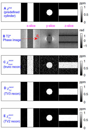
Figure 2 Scan line profiles of the numerical simulations of the cylindrical susceptibility reconstructions in . The scan line assumes a diameter of the cylinder. The ground truth is a uniform susceptibility distribution inside a cylinder, as represented by a rectangular profile.
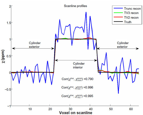
Figure 3 Numerical simulation results of BOLD fMRI with a single T2* complex image acquisition by T2*MRI (a capture of dynamic BOLD processes at one time point). The 3D data matrices (at a size of 64 × 64 × 64) are displayed with a selection of z-slices (z=10:2:32 with the central z-slice at z=32) in a montage layout: (A) the predefined susceptibility source χ (see text for vascular geometry configurations); (B) the calculated fieldmap; (C) the calculated T2* magnitude image; and (D) the calculated T2* phase image.
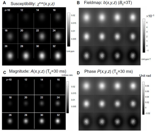
Figure 4 Numerical simulation results of magnetic susceptibility reconstructions from the T2* phase images in by two methods: filter truncation and TV iteration. Only the central z-slices (z0=32) of the 3D 64 × 64 × 64 data matrices are shown in (A). The scan line profiles extracted from the corresponding images in (A) are shown in (B). It is noted that roughness in the predefined χ map indicates the randomness of the vascular structure in the FOV (simulated with 2% filling with random beads). The ‘trunc recon’ solver produces a noisy reconstruction with an image energy shift. The ‘TV recon’ solver produces a smooth reconstruction. The correlation values between the reconstructions and the truth (0.99 for ‘TV recon’ and 0.91 for ‘trunc recon’) were calculated using Equation 18.
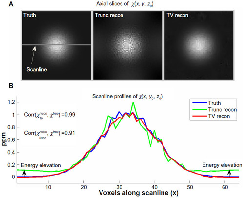
Figure 5 A typical iteration behavior of the split Bregman TV iteration algorithm (with the initial setting χ1(x, y, z) = 0).
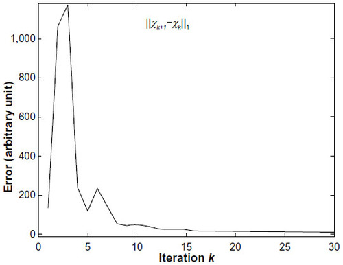
Figure 6 Magnetic susceptibility reconstructions of a phantom experiment. Experiment setting: B0=3T, FOV matrix: 32 × 32 × 32 voxels, voxel size: 3 × 3 × 3mm3, phantom: a round water tank containing a Gd-filled tube (diameter =15 mm, length =100 mm), scanning direction: B0 is perpendicular to the tube axis. The data matrices (at a size of 32 × 32 × 32) are displayed with the central z-slices (z=16) in (A) for the T2* magnitude image in dimensionless arbitrary units (au); (B) the T2* phase image in units of radian; (C) the reconstructed χ map by ‘trunc recon’; and (D) the reconstructed χ map by ‘TV recon’, where the reconstructed susceptibility values in units of ppm are different from the absolute values by an undefined constant scale. The scan line profiles from the corresponding z-slices in (A) through (D) are plotted in (E). The scan line assumes a diameter of the water container (through a plastic tube diameter as marked in B). The uniform diluted Gd solution inside the tube defines a ground truth of rectangular susceptibility distribution (normalized to [0,1] by scaling) along the scan line. The reconstructed χ values are represented in dimensionless units due to normalization. The corr values (calculated in Equation 18) represent the goodness of χ reconstructions.
![Figure 6 Magnetic susceptibility reconstructions of a phantom experiment. Experiment setting: B0=3T, FOV matrix: 32 × 32 × 32 voxels, voxel size: 3 × 3 × 3mm3, phantom: a round water tank containing a Gd-filled tube (diameter =15 mm, length =100 mm), scanning direction: B0 is perpendicular to the tube axis. The data matrices (at a size of 32 × 32 × 32) are displayed with the central z-slices (z=16) in (A) for the T2* magnitude image in dimensionless arbitrary units (au); (B) the T2* phase image in units of radian; (C) the reconstructed χ map by ‘trunc recon’; and (D) the reconstructed χ map by ‘TV recon’, where the reconstructed susceptibility values in units of ppm are different from the absolute values by an undefined constant scale. The scan line profiles from the corresponding z-slices in (A) through (D) are plotted in (E). The scan line assumes a diameter of the water container (through a plastic tube diameter as marked in B). The uniform diluted Gd solution inside the tube defines a ground truth of rectangular susceptibility distribution (normalized to [0,1] by scaling) along the scan line. The reconstructed χ values are represented in dimensionless units due to normalization. The corr values (calculated in Equation 18) represent the goodness of χ reconstructions.](/cms/asset/5abd7aa9-1979-4961-a343-af67fdb0e4d2/drmi_a_12191770_f0006_c.jpg)
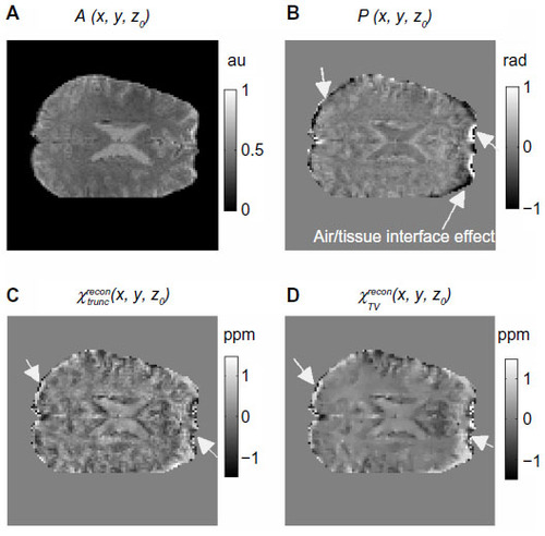
Figure 7 An in vivo brain χ tomography experiment. The MRI scanning on a healthy subject performing finger tapping in a Siemens 3T TrioTim System produced both magnitude and phase time series images (EPI sequence, TR/TE =2000/29 milliseconds, voxel =2 × 2 × 2 mm3, FOV =256 × 256 × 60 mm3), image matrix: 128 × 128 × 30. (A) Magnitude image volume at a snapshot captured at an onset =20TR in the time series dataset; (B) phase image volume (processed); (C) brain χ volume reconstructed by filter truncation solver (Equation 5, with ε0 =0.12); and (D) brain χ reconstructed by TV iteration solver (Equation 12, with λ =60 and γ1 =5).
Abbreviations: FOV, field of view; TV, total variation.
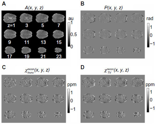
Figure 8 Display of image slices at z0=3 from volumes in : (A) magnitude image; (B) phase image (processed); (C) reconstructed χ map by filter truncation solver; and (D) reconstructed χ map by TV iteration solver. The arrows indicate air/tissue interface effects, which occur in T2* phase images and propagate to the reconstructed χ maps.