Impact of Laptev Sea flaw polynyas on the atmospheric boundary layer and ice production using idealized mesoscale simulations

Figures & data

Fig 1. (a) Consortium for Small-scale Modelling (COSMO) model domain with 15-km resolution (3000 km×3000 km, COSMO-15) and (b) the nesting domain with 5-km mesh size (1000 km×1000 km, COSMO-05). The dashed contour lines represent the topography of the model domain in metres. The polynyas from 29 April 2008 are shown as shaded areas in the 5-km model domain. The rectangle (600 km×600 km) in (b) sketches the area of main interest and indicates the locations of the polynyas we refer to in our studies as P1 (the Anabar–Lena polynya) and P2 (the western New Siberian polynya) as well as the locations of the Taimyr Peninsula (TP) and the Lena Delta (LD).

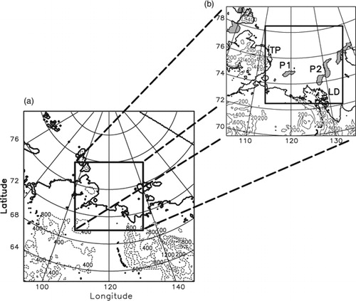
Fig 2. The schematic shows the design used in our study. The Consortium for Small-scale Modelling (COSMO) module ‘src_artifdata.f90’ provides the idealized atmospheric conditions. Regimes are shown in Fig. 3 and Table 2.

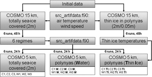
Fig 3. Initial conditions for COSMO-05 obtained from six different COSMO-15 simulations: (a) C1, (b) W1, (c) C2, (d) W2, (e) C3 and (f) W3. Cold regimes are illustrated in (a), (c) and (e) and warm regimes in (b), (d) and (f). The surface temperature is represented by the dashed contour lines with 1-K intervals. Contour minimum for the cold cases is −39°C and for the warm cases −32°C. Vectors indicate 10-m wind velocity (ms⁻¹; every eighth component in meridional [v] and zonal [u] directions). Grey shading indicate the polynya locations (see Fig. 1). The small rectangle in (f) is used to obtain the characteristic properties (10-m wind speed and sea-ice surface temperature) for each simulation (see Table 2). The dot in the centre of the small rectangle marks the position of the profiles shown in Fig. 4.

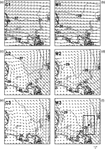
Table 1. Initial, constant and boundary fields for the idealized Consortium for Small-scale Modelling (COSMO) studies.

Parameter	Derived from
Elevation	Global Land One-Kilometre Base Elevation (GLOBE) digital elevation model (1 km; Hastings et al. 1999)
Land cover	GLOBE data set
Soil type	National Aeronautical and Space Administration (5 km; Zobler 1986)
Sea-ice coverage	Advanced Microwave Scanning Radiometer–Earth Observing System (6.25 km; Spreen et al. 2007)
Plant cover	Satellite data with 10′ resolution (Kineman & Hastings 1992)
Leaf area index	Plant cover larger than 0 has a leaf area index=1
Root depth	Global Model Extended (GME; 40 km)
Roughness length	Land: GME (40 km); sea ice: z 0=10^−3 m; water: Charnock (1955)
Soil properties	GME (40 km)
Sea-ice properties	Sea-ice surface temperature: −20.2°C/−30.2°C, water: constant at −1.7°C
Atmosphere	Prescribed in artifdata module of COSMO

Table 2. Start conditions of COSMO-15 and COSMO-05 simulations for cold (C1–C3) and warm regimes (W1–W3). Initial wind speed (v) for COSMO-15 runs applied for all models layers and ice surface temperatures (IST) for the whole sea-ice cover. IST and 10-m wind speed (v_10) as area mean averages of COSMO-05 are from the rectangle in Fig. 3f.

Cold regimes					Warm regimes
	COSMO-15		COSMO-05		COSMO-05		COSMO-15
Regime	IST (°C)	v (ms^−1)	IST (°C)	v_10 (ms^−1)	IST (°C)	v_10 (ms^−1)	IST (°C)	v (ms^−1)	Regime
C1	−30.2	15	−37.3	7.6	−29.7	7.6	−20.2	15	W1
C2	−30.2	4	−37.3	6.8	−29.4	6.3	−20.2	4	W2
C3	−30.2	3	−37.1	4.2	−29.2	4.6	−20.2	3	W3

Fig 4. (a) Potential temperature (θ) in °C (solid lines) and specific humidity (q) in g kg⁻¹ (dashed line, upper axis). (b) Wind speed (ff) in ms⁻¹ (solid line) and wind direction (dd) in degrees (dashed line, upper axis). Open circles represent regime C1; closed circles represent regime W3 (Fig. 3, Table 2). Profiles were obtained at the position masked by the dot in Fig. 3f.

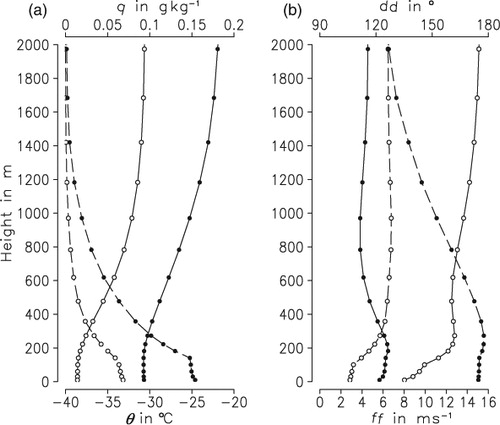
Fig 5. Atmospheric conditions after 24-h simulation with COSMO-05 for the cold regimes and ice-free polynyas (see initial conditions in Fig. 3). (a), (c), (e) Ten-m wind vectors (every eighth grid point) in ms⁻¹ and 2-m air temperature (2-K intervals between dashed contour lines; minimum contour values −44°C). (b), (d), (f) Anomalies between simulations with polynyas and 100% sea-ice cover after a simulation time of 24 h, with 10-m wind vectors (every fourth grid point) in ms⁻¹. Wind speed anomalies of less than 1 ms⁻¹ are masked out.

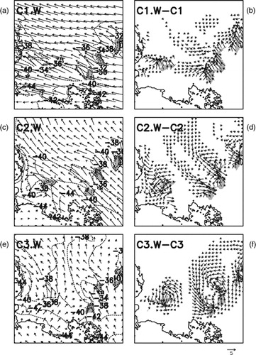
Fig 6. Atmospheric conditions after 24-h simulation with COSMO-05 for the warm regimes and ice-free polynyas (see initial conditions in Fig. 3). (a), (c), (e) Ten-m wind vectors (every eighth grid point) in ms⁻¹ and 2-m air temperature (2-K intervals between dashed contour lines; minimum contour values −40°C). (b), (d), (f) Anomalies between simulations with polynyas and 100% sea-ice cover after a simulation time of 24 h, with 10-m wind vectors (every fourth grid point) in ms⁻¹. Wind speed anomalies of less than 1 ms⁻¹ are masked out.

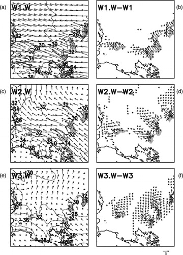
Fig 7. Differences of temperature (shaded) in K between simulations with polynyas and a wholly sea-ice covered Laptev Sea. For location see Fig. 1b. (a), (d), (g) Two-m temperature anomalies in K (shaded) overlaid with horizontal 10-m wind vectors in ms⁻¹ and maximum cloud coverage of the lower 2000 m (light/dark blue contour lines indicate cloud coverage of 10% and 90%). The thick black line sketches the position of the vertical cross-section shown in (b), (e), (h) for cold regimes and in (c), (f), (i) for warm regimes: Temperature anomalies in K (shaded) plotted with potential temperatures (θ) indicated by thin black contour lines with 1-K intervals. The thick black curve marks the 0.01 g kg⁻¹ isoline for specific humidity and the light/dark blue curves mark the cloud coverage isoline of 10%/90%, respectively. The grey line on the x-axis marks the sea-ice cover.

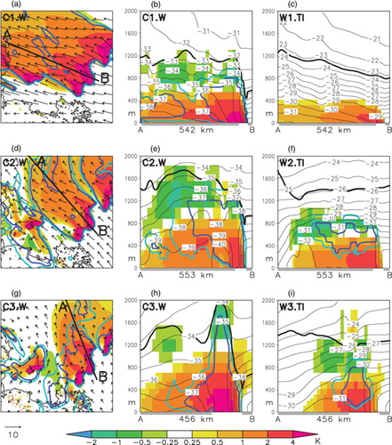
Fig 8. Differences of temperature (shaded) in K between simulations with open-water polynyas and a wholly sea-ice covered Laptev Sea. For location see Fig. 1b. (a) Two-m temperature anomalies in K (shaded) overlaid with horizontal 10-m wind vectors in ms⁻¹ and maximum cloud coverage of the lower 2000 m (light/dark blue contour lines indicate cloud coverage of 10% and 90%). The thick black line sketches the position of the vertical cross-section shown in (b) for the cold regime and in (c) for the warm regime: temperature anomalies in K (shaded) plotted with potential temperatures (θ) indicated by thin black contour lines with 1-K intervals (as in Fig. 7). The thick black curve marks the 0.01 g kg⁻¹ isoline for specific humidity and the light/dark blue curves mark the cloud coverage isoline of 10%/90%, respectively. The grey line on the x-axis marks the sea-ice cover.

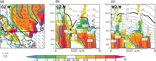
Table 3. Total surface turbulent heat flux (latent [E₀] plus sensible [H₀] heat) and Bowen ratio (β) for polynya P2 (Fig. 1b). Mean area and time averaged values over a simulation time of 24 h.

Regime	Water W m^−2	β=H0/E0	Thin ice W m^−2	β=H0/E0	Δ W m^−2
C1	−619	4.3	−345	8.6	−274
C2	−479	4.6	−308	8.8	−171
C3	−340	4.4	−219	7.3	−121
W1	−470	3.5	−265	5.8	−205
W2	−357	3.8	−223	6.1	−134
W3	−240	3.7	−156	5.5	−84

Table 4. Surface net radiation flux (Q₀) for polynya P2 (Fig. 1b). Mean area and time averaged values over a simulation time of 24 h.

Regime	Water W m^−2	Thin ice W m^−2	Δ W m^−2
C1	−170	−173	+3
C2	−154	−157	+3
C3	−152	−141	−9
W1	−192	−173	−19
W2	−170	−167	−3
W3	−160	−158	−2

Fig 9. Two-m air temperature in °C and 10-m wind speed (contours have 1 ms⁻¹ intervals) as obtained after a simulation time of 24 h for (a) and (b) polynya P2 and (c) and (d) polynya P1. Regime C1.W, with an ice-free polynya, is represented in (a), while regime W3.TI, with 5-cm thin ice is shown in (b). For location see Fig. 1b. The areal extent of (a) and (b) is 150 km×250 km and of (c) and (d) is 150 km×100 km.

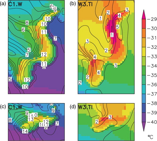
Fig 10. Potential sea-ice production rates in cm d⁻¹ (shaded) of the polynya areas P1 and P2 (see Fig. 1b) after a simulation time of 24 h and 10-m wind vectors (ms⁻¹). (a), (b), (c) Potential ice production with open-water polynyas and cold regimes (C1.W, C2.W, C3.W). (d), (e), (f) Potential ice production with open-water polynyas and warm regimes (W1.W, W2.W, W3.W). Potential sea-ice production rates (h) in cm d⁻¹ and sea-ice volume production (V) in km³ d⁻¹ are calculated as an area and time average over 24 h for the polynyas (left value=P1, right value=P2).

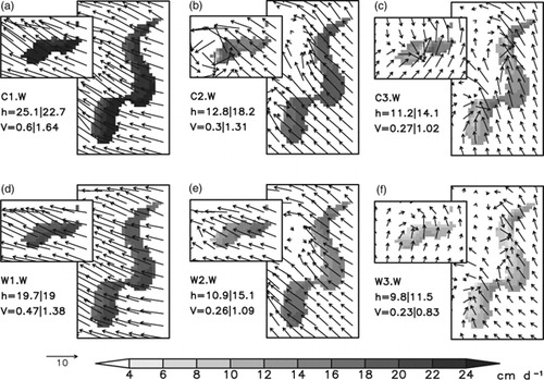
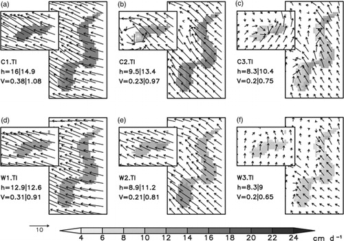
Fig 11. Potential sea-ice production rates in cm d⁻¹ (shaded) of the polynya areas P1 and P2 (see Fig. 1b) after a simulation time of 24 h and 10-m wind vectors (ms⁻¹). (a), (b), (c) Potential ice production with thin ice covered polynyas and cold regimes (C1.TI, C2.TI, C3.TI). (d), (e), (f) Potential ice production with thin ice covered polynyas and warm regimes (W1.TI, W2.TI, W3.TI). Potential sea-ice production rates (h) in cm d⁻¹ and sea-ice volume production (V) in km³ d⁻¹ are calculated as an area and time average over 24 h for the polynyas (left value=P1, right value=P2).

Hastings D. A., Dunbar P.K., Elphingstone G.M., Bootzan M., Murakami H., Maruyama H., Masaharu H., Holland P., Payne J., Bryant N.A., Logan T.L., Muller J.-P., Schreier G. & MacDonald J.S. (eds.) 1999. The Global Land One-Kilometre Base Elevation (GLOBE) digital elevation model. Version 1.0. Boulder, CO: National Geophysical Data Centre, National Oceanic and Atmospheric Administration.

 Google Scholar

Zobler L. 1986. A world soil file for global climate modelling. NASA Technical Memorandum 87802. Washington, DC: National Aeronautical and Space Administration.

 Google Scholar

Spreen G., Kaleschke L. & Heygster G. 2007. Sea ice remote sensing using AMSR—E 89 GHz channels. Journal of Geo-physical Research—Oceans 113, CO2503, doi: 10.1029/2005JC003384.

 Google Scholar

Kineman J. & Hastings D. 1992. Monthly generalized global vegetation index from NESDIS NOAA-9 weekly GVI data (Apr 1985-Dec 1988). Boulder, CO: National Geophysical Data Centre, National Oceanic and Atmospheric Administration.

 Google Scholar

Charnock H. 1955. Wind stress over a water surface. The Quarterly Journal of the Royal Meteorological Society 81, 639–640.

 Web of Science ®Google Scholar