Figures & data
Fig. 1 Mean vertical profiles of CO of MOZAIC and TES observations are plotted along with standard deviation for different seasons (DJF, MAM, JJA and SON) during a 5-yr period (2006–2010). N represents the total number of profiles.
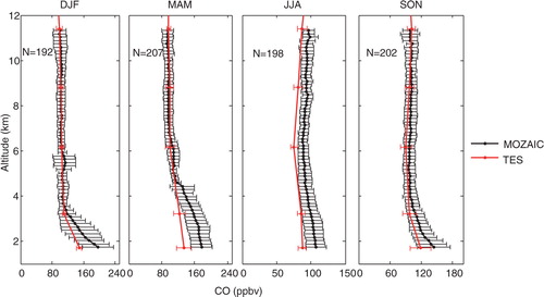
Fig. 2 Mean vertical profiles of O3 of MOZAIC and TES observations are plotted along with standard deviation for different seasons (DJF, MAM, JJA and SON) during a 5-yr period (2006–2010). N represents the total number of profiles.
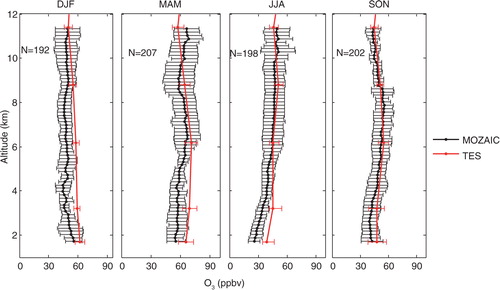
Table 1. Mean bias between TES and MOZAIC observations for four seasons DJF, MAM, JJA and SON is calculated at different tropospheric altitude regions
Fig. 3 Monthly mean anomalies of CO are shown over Hyderabad in the three tropospheric layers with MOZAIC (0–2, 2–8 and 8–10 km) and TES (2–8 km) observations. N and p represent the total number of MOZAIC profiles and p value, respectively.
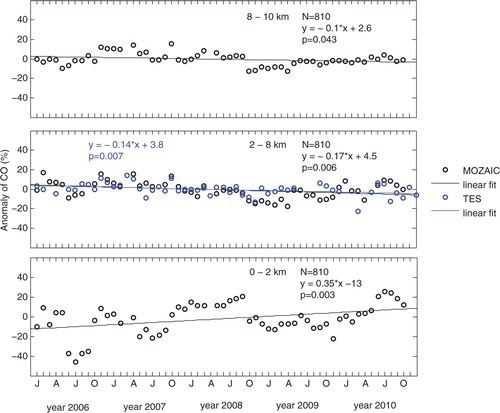
Fig. 4 Monthly mean anomalies of O3 are shown over Hyderabad in the three tropospheric layers with MOZAIC (0–2, 2–8 and 8–10 km) and TES (2–8 km) observations. N and p represents the total number of MOZAIC profiles and p value, respectively.
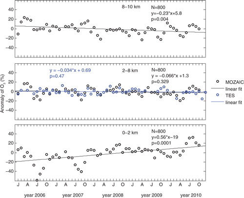
Table 2. Changes in CO and O3 obtained from MOZAIC observations with respect to the year 2006 in Hyderabad
Fig. 5 Monthly mean profiles of CO along with standard deviation are plotted for different months of the year 2009 for MOZAIC observations and WRF-Chem and MOZART-4 simulations. N represents the total number of profiles of that particular month.
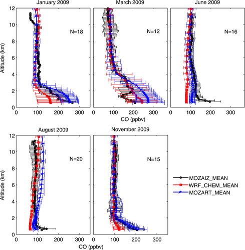
Fig. 6 Monthly mean profiles of O3 along with standard deviation are plotted for different months of the year 2009 for MOZAIC observations and WRF-Chem and MOZART-4 simulations. N represents the total number of profiles of that particular month.
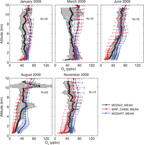
Table 3. Mean bias is calculated for monthly average WRF-Chem and MOZART-4 simulated CO and O3 with respect to MOZAIC observations for different months of the year 2009.
Fig. 7 The monthly mean MOZAIC CO profiles (MOZAIC_MEAN) for 5 months of the year 2009 are shown along with the standard deviation. The anomalous profile observed by MOZAIC for a particular month is shown along with the spatially and temporarily collocated profile simulated by WRF-Chem using BMJ, KF and GD convection schemes and MOZART-4 model.
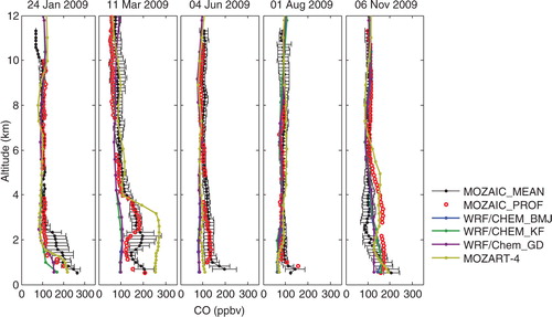
Table 4. Mean bias in O (CO) for the anomalous profiles of the year 2009 is calculated at different layers of the troposphere
Fig. 9 MOZAIC observed temperature (bottom x-axis labels) and water vapour mixing ratio (top x-axis labels) profiles are plotted along with WRF-Chem simulation corresponding to CO and O3 anomalous profiles.
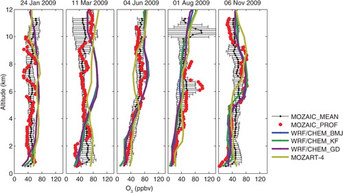
Fig. 10 MOZAIC observed and WRF-Chem simulated wind speed profiles are plotted corresponding to anomalous CO and O3 profiles.
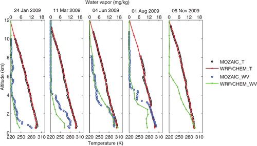
Fig. 11 Wind direction corresponding to anomalous CO and O3 profiles obtained from MOZAIC observation and WRF-Chem simulations are plotted against altitude.
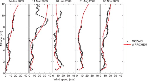
Fig. 12 WRF-Chem winds are plotted overlaid on O3 (ppbv) at 2, 6 and 8 km altitude region at 6, 12 and 18 GMT. The O3 over Hyderabad lies inside the box in the figure.
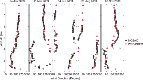
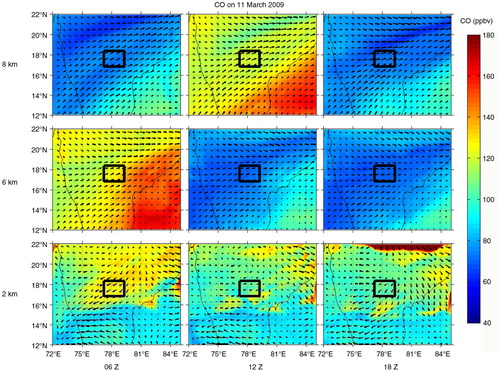
Fig. 13 WRF-Chem winds are plotted overlaid on CO (ppbv) at 2, 6 and 8 km altitude regions at 6, 12 and 18 GMT. The CO over Hyderabad lies inside the box in the figure.
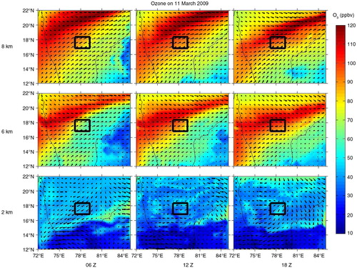
Table 5. Mean bias is calculated for WRF-Chem with respect to MOZAIC observations for temperature, water vapour mixing ratio and wind speed at different altitude region
Fig. 8 The monthly mean MOZAIC O3 profiles (MOZAIC_MEAN) for 5 months of the year 2009 are shown along with the standard deviation. The anomalous profile observed by MOZAIC for a particular month is shown along with the spatially and temporarily collocated profile simulated by WRF-Chem using BMJ, KF and GD convection schemes and MOZART-4 model.