p-Values, Bayes Factors, and Sufficiency

ABSTRACT

Various approaches can be used to construct a model from a null distribution and a test statistic. I prove that one such approach, originating with D. R. Cox, has the property that the p-value is never greater than the Generalized Likelihood Ratio (GLR). When combined with the general result that the GLR is never greater than any Bayes factor, we conclude that, under Cox’s model, the p-value is never greater than any Bayes factor. I also provide a generalization, illustrations for the canonical Normal model, and an alternative approach based on sufficiency. This result is relevant for the ongoing discussion about the evidential value of small p-values, and the movement among statisticians to “redefine statistical significance.”

KEYWORDS:

• Embedding model
• Exponential tilting
• Generalized Likelihood Ratio (GLR)

1. Outline

This is a brief contribution to the ongoing discussion about the evidential import of a small p-value (see, e.g., Wasserstein and Lazar 2016). Let $X\in \mathcal{X}$ be a set of observables, and H₀: X ∼ f₀ be a null distribution. A “significance procedure” for H₀ is any statistic $p_0:\mathcal{X}\to \mathbb{R}$ such that p₀(X) under H₀ stochastically dominates a uniform distribution. If p₀ is a significance procedure for H₀, then $p_0\left(x^{\text{obs}}\right)$ is a “p-value” for H₀, where $x^{\text{obs}}$ are the observations of X. The usual way to construct a significance procedure is to propose a test statistic $t:\mathcal{X}\to \mathbb{R}$. Then (1) $$p_0\left(x\right):=P{r}_0\{t\left(X\right)\ge t\left(x\right)\}$$(1) is a significance procedure according to the Probability Integral Transform, where Pr₀ is the probability under H₀. For more on these definitions see, for example, Casella and Berger (2002, sec. 8.3) and Lehmann and Romano (2005, chap. 9). The distinction between a “procedure” and a “value,” which I have taken from Morey et al. (2016), is very useful in practice.

The critical issue is whether it is advisable to dismiss the null distribution on the basis of a small p-value, without explicitly considering any alternatives. The article addresses this issue by producing and justifying an “embedding model” based on the null distribution and the test statistic, in which the null distribution is at one end of the parameter space of the embedding model (Section 2). Within this embedding model (2) $$p_0\left(x\right)\le G_{01}\left(x\right)\le B_{01}\left(x\right),$$(2) where G₀₁ is the Generalized Likelihood Ratio (GLR) and B₀₁ is the Bayes factor. It follows from these inequalities that evidential thresholds for Bayes factors or GLRs translate into evidential thresholds for p-values. For example, if we accepted Harold Jeffreys’s threshold that B₀₁(x) = 10^{− 3/2} ≈ 0.032 separates “strong” from “very strong” evidence against the null distribution, then p₀(x) ⩽ 0.032 would be the most lenient possible threshold for p-values designed to detect “very strong” evidence against the null distribution. This is less than the conventional threshold of p₀(x) ⩽ 0.05, but not by much; although even a small difference would have a substantial impact in some fields (Masicampo and Lalande 2012).

On the other hand, for a specific null distribution and test statistic, we can construct the embedding model and evaluate the exact relationship between the p-value and the GLR. In the canonical case where the embedding model is Normal (Section 3), a p-value of 0.05 corresponds to a GLR of 0.259, and a GLR of 0.032 corresponds to a p-value of 0.004. So in this case, accepting Jeffreys’s threshold would lead to p₀(x) ⩽ 0.004 as the most lenient possible threshold for p-values. This is close to the suggestion of p₀(x) ⩽ 0.005, made by Johnson (2013). This threshold of p₀(x) ⩽ 0.005 has recently been advocated by a large group of statisticians (Benjamin et al. 2018), and questioned by another large group of statisticians (Lakens et al. 2018).

Section 4 provides a different justification for (2(2) $$p_0\left(x\right)\le G_{01}\left(x\right)\le B_{01}\left(x\right),$$(2) ) via the sufficiency of the test statistic in the embedding model, which holds when the components of X are independent and identically distributed (IID).

2. D. R. Cox’s Embedding Model

The attraction of a significance procedure is that it does not require a model for X within which the null distribution is a single element. Any attempt to link p-values with GLRs and Bayes factors must produce such a model based, as far as possible, only on the ingredients to hand: the null distribution and the test statistic. Clearly these two components are insufficient, and some additional principle must be used to justify any particular choice.

One principle is to assume that the test statistic t was carefully chosen to reflect the question of interest. This suggests an embedding model for X in which t is an unambiguously good choice for testing H₀ versus “not H₀,” as was originally proposed by D. R. Cox, in Savage et al. (1962, p. 84) and Cox (1977). Cox proposed the exponentially tilted embedding model (3) $$f(x;\theta )=\frac{f_0\left(x\right)·e^{\theta ·t\left(x\right)}}{M_T\left(\theta \right)},\theta \ge 0,$$(3) where M_T is the moment generating function of t(X) under H₀. This model has a monotone likelihood ratio in t(x), and hence the test statistic t is uniformly most powerful (UMP) in testing H₀: θ = 0 versus H₁: θ > 0 (see, e.g., Casella and Berger 2002, sec. 8.3).

This is a “sufficient” argument for (3(3) $$f(x;\theta )=\frac{f_0\left(x\right)·e^{\theta ·t\left(x\right)}}{M_T\left(\theta \right)},\theta \ge 0,$$(3) ) as the embedding model; that is, were (3(3) $$f(x;\theta )=\frac{f_0\left(x\right)·e^{\theta ·t\left(x\right)}}{M_T\left(\theta \right)},\theta \ge 0,$$(3) ) the model, then t would be the analyst’s unambiguous choice of test statistic for H₀ versus “not H₀.” But it is also hard to imagine a simpler way to create an embedding model out of just f₀ and t, and this might be a more practical justification for (3(3) $$f(x;\theta )=\frac{f_0\left(x\right)·e^{\theta ·t\left(x\right)}}{M_T\left(\theta \right)},\theta \ge 0,$$(3) ). However, Section 4 presents another justification with strong intuitive appeal. I will refer to (3(3) $$f(x;\theta )=\frac{f_0\left(x\right)·e^{\theta ·t\left(x\right)}}{M_T\left(\theta \right)},\theta \ge 0,$$(3) ) as the “ET” (exponentially tilted) embedding model.

Initially, consider the Bayes factor for H₀ versus H₁, (4) $$B_{01}\left(x\right):=\frac{f_0\left(x\right)}{{\int }_0^{\infty }f(x;\theta )\pi \left(\theta \right)d\theta },$$(4) where π is some prior distribution on θ ∈ (0, ∞). Adopting the approach originally proposed by Edwards, Lindman, and Savage (1963, p. 228), the Bayes factor can be bounded below over the set of all possible priors, (5) $$\begin{array}{ccc}\hfill B_{01}\left(x\right)& \ge & \underset{\pi }{inf}\frac{f_0\left(x\right)}{{\int }_0^{\infty }f(x;\theta )\pi \left(\theta \right)d\theta }\hfill \\ & =& \frac{f_0\left(x\right)}{{sup}_{\theta >0}f(x;\theta )}=:G_{01}\left(x\right),\hfill \end{array}$$(5) where G₀₁ is the GLR. This simple result is true for every embedding model. But then, using the ET embedding model in (3(3) $$f(x;\theta )=\frac{f_0\left(x\right)·e^{\theta ·t\left(x\right)}}{M_T\left(\theta \right)},\theta \ge 0,$$(3) ), (6) $$\begin{array}{ccc}\hfill G_{01}\left(x\right)& =& \underset{\theta >0}{inf}\frac{f_0\left(x\right)}{f(x;\theta )}\hfill \\ & =& \underset{\theta >0}{inf}{e}^{-\theta ·t\left(x\right)}{M}_T\left(\theta \right)\hfill \\ & \ge & P{r}_0\{t\left(X\right)\ge t\left(x\right)\}\hfill \\ & =& p_0\left(x\right)\hfill \end{array}$$(6) according to Chernoff’s inequality (e.g., Whittle 2000, chap. 15). Chernoff’s inequality is an application of Markov’s inequality, and therefore in principle it is tight, but in practice an equality would be very unusual for a statistical model. One exception is when the components of X are IID and t(x) = x₁ + … + x_n, in which case (6(6) $$\begin{array}{ccc}\hfill G_{01}\left(x\right)& =& \underset{\theta >0}{inf}\frac{f_0\left(x\right)}{f(x;\theta )}\hfill \\ & =& \underset{\theta >0}{inf}{e}^{-\theta ·t\left(x\right)}{M}_T\left(\theta \right)\hfill \\ & \ge & P{r}_0\{t\left(X\right)\ge t\left(x\right)\}\hfill \\ & =& p_0\left(x\right)\hfill \end{array}$$(6) ) is asymptotically exact; this is a result from Large Deviation Theory (see, e.g., Whittle 2000, chap. 18).

Putting the inequalities (5(5) $$\begin{array}{ccc}\hfill B_{01}\left(x\right)& \ge & \underset{\pi }{inf}\frac{f_0\left(x\right)}{{\int }_0^{\infty }f(x;\theta )\pi \left(\theta \right)d\theta }\hfill \\ & =& \frac{f_0\left(x\right)}{{sup}_{\theta >0}f(x;\theta )}=:G_{01}\left(x\right),\hfill \end{array}$$(5) ) and (6(6) $$\begin{array}{ccc}\hfill G_{01}\left(x\right)& =& \underset{\theta >0}{inf}\frac{f_0\left(x\right)}{f(x;\theta )}\hfill \\ & =& \underset{\theta >0}{inf}{e}^{-\theta ·t\left(x\right)}{M}_T\left(\theta \right)\hfill \\ & \ge & P{r}_0\{t\left(X\right)\ge t\left(x\right)\}\hfill \\ & =& p_0\left(x\right)\hfill \end{array}$$(6) ) together, (3(3) $$f(x;\theta )=\frac{f_0\left(x\right)·e^{\theta ·t\left(x\right)}}{M_T\left(\theta \right)},\theta \ge 0,$$(3) ) implies (2(2) $$p_0\left(x\right)\le G_{01}\left(x\right)\le B_{01}\left(x\right),$$(2) ). Thus, if the embedding model is the ET embedding model, then the p-value for H₀ is never greater than the GLR for H₀ versus H₁, which is never greater than the Bayes factor for H₀ versus any alternative in the embedding model. It is superficially puzzling that two constructions which seem fundamentally different can be ordered by their values. But, on the one hand, the modern definition of a significance procedure p₀ implies that p₀(y) ∈ (0, ∞), just like a Bayes factor. On the other hand, the ET embedding model ensures that B₀₁(y) ∈ [0, 1], just like a probability.

Curious readers will be wondering how close Wilks’s p-value is to its upper bound of G₀₁(x), under the ET embedding model. Wilks’s theorem states that (7) $$-2log{G}_{01}\left(X\right)\underset{\phantom{1.25cm}}{\overset{\mathrm{D}}{\to }}{\chi }_1^2\text{under}{H}_0\text{and}\text{(3),}$$(7) if the components of X are IID (plus other technical conditions: see, e.g., Casella and Berger 2002, sec. 10.3). 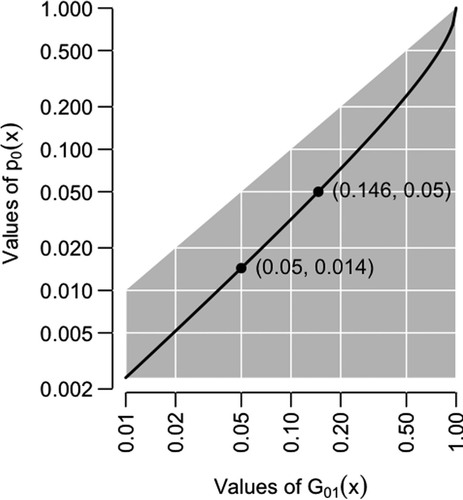Thus, each value of G₀₁(x) can be mapped to a p-value for H₀: (8) $$p_0\left(x\right)=Pr\{{\chi }_1^2\ge -2log{G}_{01}\left(x\right)\},$$(8) where p₀ is an approximate significance procedure for finite n. Figure 1 shows the result: a Wilks’s p-value of 0.05 corresponds to a GLR of 0.146. In other words, the IID and n → ∞ conditions on X have reduced the p-value by as much as 10 percentage points. As this example illustrates, it is always pertinent to ask whether it is the observations or the conditions which produce a small p-value.

Figure 1. The GLR and Wilks’s p-value. The gray region shows the possible values of p₀ under the ET embedding model given in (3(3) $$f(x;\theta )=\frac{f_0\left(x\right)·e^{\theta ·t\left(x\right)}}{M_T\left(\theta \right)},\theta \ge 0,$$(3) ), and the solid line the values of Wilks’s p-value, based on the asymptotic distribution of − 2log G₀₁(X) under the null distribution.

Finally, note that the ET embedding model can be generalized to (9) $$f(x;\varphi )\propto f_0\left(x\right)·e^{\varphi ·h\left(t\right(x\left)\right)},\varphi \ge 0,$$(9) for any increasing h without t losing its UMP property, for which (6(6) $$\begin{array}{ccc}\hfill G_{01}\left(x\right)& =& \underset{\theta >0}{inf}\frac{f_0\left(x\right)}{f(x;\theta )}\hfill \\ & =& \underset{\theta >0}{inf}{e}^{-\theta ·t\left(x\right)}{M}_T\left(\theta \right)\hfill \\ & \ge & P{r}_0\{t\left(X\right)\ge t\left(x\right)\}\hfill \\ & =& p_0\left(x\right)\hfill \end{array}$$(6) ) still holds, and (2(2) $$p_0\left(x\right)\le G_{01}\left(x\right)\le B_{01}\left(x\right),$$(2) ) likewise. H replaces T, and the final step is (10) $$P{r}_0\{h\left(t\left(X\right)\right)\ge h\left(t\left(x\right)\right)\}=P{r}_0\{t\left(X\right)\ge t\left(x\right)\}=p_0\left(x\right)$$(10) because h is increasing. Therefore, the ET embedding model is more properly thought of as a class of embedding models, and the inequalities in (2(2) $$p_0\left(x\right)\le G_{01}\left(x\right)\le B_{01}\left(x\right),$$(2) ) hold for every embedding model in the class.

3. Illustration: The Normal Model

To illustrate both inequalities in (2(2) $$p_0\left(x\right)\le G_{01}\left(x\right)\le B_{01}\left(x\right),$$(2) ), consider the canonical statistical model, first analyzed in this context by Edwards, Lindman, and Savage (1963, p. 228). Let the null distribution be X ∼ N(0, σ²) for known σ, where I take σ = 1 for simplicity and without loss of generality. Let the test statistic be t(x) = x. Then the ET embedding model is X ∼ N(θ, 1), for which H₀: θ = 0 versus H₁: θ > 0 is a conventional one-tailed test for location. The GLR is (11) $$G_{01}\left(x\right)=\left\{\begin{array}{cc}\hfill 1& \hfill x\le 0\\ \hfill e^{-\frac{1}{2}{x}^2}& \hfill x>0.\end{array}\right.$$(11) The p-value is a deterministic function of x, from which it is possible to plot G₀₁, the lower bound for B₀₁, as a deterministic function of p₀, as shown in Figure 2.

Figure 2. The Generalized Likelihood Ratio G₀₁ and possible Bayes factors B₀₁ (gray region), as functions of the p-value p₀, for the null distribution X ∼ N(0, 1) and the test statistic t(x) = x, which is a UMP one-tailed test for location.

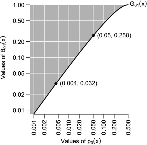
Figure 2 also shows some specific values: the lower bound on B₀₁(x) when p₀(x) = 0.05, and the value of p₀(x) corresponding to a lower bound of B₀₁(x) = 10^{− 3/2} ≈ 0.032, which is the boundary between “strong” and “very strong” evidence against H₀ in the scheme of Jeffreys (1961, see Appendix B). In this example, a p-value at the conventional threshold of 0.05 corresponds to a lower bound on the Bayes factor of 0.259: “Even the utmost generosity to the alternative hypothesis cannot make the evidence in favor of it as strong as classical significance levels might suggest” (Edwards, Lindman, and Savage 1963, p. 228). From the other direction, the necessary condition for satisfying Jeffreys’s boundary is p₀(x) ⩽ 0.004. Jeffreys’s boundary is only a convention, but the sizable absolute discrepancy between the two points in Figure 2, on either scale, casts doubt on the advisability of dismissing the null distribution for a p-value of about 0.05.

In this illustration, the null distribution, test statistic, and ET embedding model combined can give a UMP one-tailed test for location. It is natural to ask whether a different choice of test statistic can give a two-tailed test for location, but the answer must be negative because there is no UMP two-tailed test for location (see, e.g., Casella and Berger 2002, sec. 8.3). It follows that “two-tailed” test statistics might have unexpected ET embedding models.

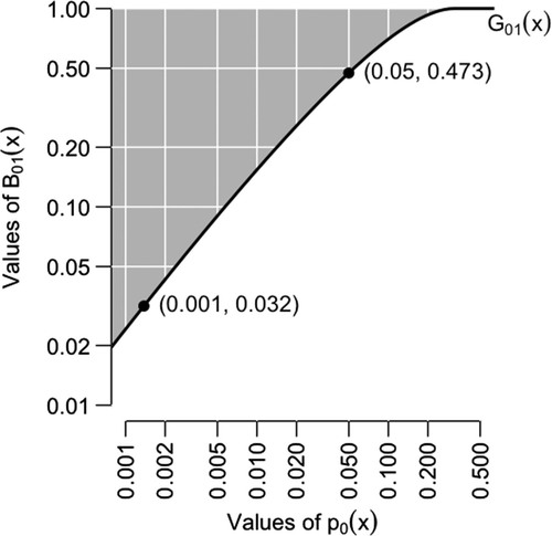
To illustrate, if t(x) = x², which is large in both tails of the null distribution, then the ET embedding model is equivalent to (12) $$X\sim N(0,1+\theta ),$$(12) showing that x² is a UMP one-tailed test for dispersion. The GLR for this model is (13) $$G_{01}\left(x\right)=\left\{\begin{array}{cc}\hfill 1& \hfill \left|x\right|\le 1\\ \hfill \left|x\right|·e^{-\frac{1}{2}(x^2-1)}& \hfill \left|x\right|>1.\end{array}\right.$$(13) The relationship between the p-value and the GLR is shown in Figure 3. This figure carries a similar message to Figure 2, which is that there is a large difference between the p-value and the Bayes factor. A p-value at the conventional threshold of 0.05 corresponds to a lower bound on the Bayes factor of 0.473, which is very weak evidence against the null distribution. The necessary condition for satisfying Jeffreys’s condition of B₀₁(x) ⩽ 0.032 is p₀(x) ⩽ 0.001, to three decimal places.

Figure 3. Similar to Figure 2, except based on the “two-tailed” test statistic t(x) = x², which is a UMP one-tailed test for dispersion.

In both of these illustrations, we could have chosen nonlinear increasing functions of the test statistic to use in the ET embedding model. For example, x³ in the first illustration, and x⁴ in the second. This changes the ET embedding model, and therefore the implicit hypothesis test for which t(x) is UMP. It also changes the GLR. But it does not change the p-value, and it does not change the result that the p-value is never greater than the GLR (see the end of Section 2). The absolute size of the gap between the p-value and the GLR can only be assessed with respect to a specific choice of test statistic.

4. Justification via Sufficiency

The weakness of the argument in Section 2 is that it relies on exponential tilting to construct the embedding model given in (3(3) $$f(x;\theta )=\frac{f_0\left(x\right)·e^{\theta ·t\left(x\right)}}{M_T\left(\theta \right)},\theta \ge 0,$$(3) ), or its generalization in (9(9) $$f(x;\varphi )\propto f_0\left(x\right)·e^{\varphi ·h\left(t\right(x\left)\right)},\varphi \ge 0,$$(9) ), and it loses its force when the analyst does not think that exponential tilting is appropriate. There is an another argument which can be applied in the case where the components of X are IID. The crux of this argument is to arrive at (9(9) $$f(x;\varphi )\propto f_0\left(x\right)·e^{\varphi ·h\left(t\right(x\left)\right)},\varphi \ge 0,$$(9) ) using a sufficiency principle.

We require a one-dimensional version of the Pitman–Koopmans–Darmois (PKD) theorem, which was originally sketched in Fisher (1934), with a modern proof in Schervish (1995, sec. 2.2.3). This theorem validates the following result (plus some technical conditions not given here). If

1.	the components of X are IID,
2.	the support of the embedding model is constant, and
3.	the test statistic is sufficient in the embedding model,

then (14) $$f(x;\varphi )\propto f_0\left(x\right)·e^{\varphi ·h\left(t\right(x\left)\right)},$$(14) where h is invertible, and the boundary condition f(x; 0) = f₀(x) has been imposed. To orient this model so that large values of the test statistic challenge the null distribution, we take φ ⩾ 0 and h increasing, similar to (9(9) $$f(x;\varphi )\propto f_0\left(x\right)·e^{\varphi ·h\left(t\right(x\left)\right)},\varphi \ge 0,$$(9) ). Then the argument in Section 2 goes through exactly as before.

Acknowledgments

The author thanks Patrick Rubin-Delanchy and Christian Robert for their helpful comments on previous versions of this article; and a TAS reviewer, whose detailed comments on two versions of this article resulted in many improvements.

Funding

This research was supported by the EPSRC SuSTaIn Grant, reference EP/D063485/1.

References

- Benjamin, D. et al., (2018), “Redefine Statistical Significance,” Nature Human Behaviour, 2, 6–10.
- Casella, G., and Berger, R. (2002), Statistical Inference (2nd ed.), Pacific Grove, CA: Duxbury.
- Cox, D. (1977), “The Role of Significance Tests” (with discussion and rejoinder), Scandinavian Journal of Statistics, 4, 49–70.
- Edwards, W., Lindman, H., and Savage, L. (1963), “Bayesian Statistical Inference for Psychological Research,” Psychological Review, 70, 193–242.
- Fisher, R. (1934), “Two New Properties of Mathematical Likelihood,” Proceedings of the Royal Society, Series A, 144, 285–307.
- Jeffreys, H. (1961), Theory of Probability (3rd ed.), Oxford, UK: Oxford University Press.
- Johnson, V. (2013), “Revised Standards for Statistical Evidence,” Proceedings of the National Academy of Sciences, 110, 19313–19317.
- Lakens, D., et al. (2018), “Justify Your Alpha,” Nature Human Behaviour, 2, 168–171.
- Lehmann, E., and Romano, J. (2005), Testing Statistical Hypotheses (3rd ed.), New York: Springer.
- Masicampo, E., and Lalande, D. (2012), “A Peculiar Prevalence of p Values just Below .05,” The Quarterly Journal of Experimental Psychology, 65, 2271–2279.
- Morey, R., Hoekstra, R., Rouder, J., Lee, M., and Wagenmakers, E.-J. (2016), “The Fallacy of Placing Confidence in Confidence Intervals,” Psychonomic Bulletin & Review, 23, 103–123.
- Savage, L., et al. (1962), The Foundations of Statistical Inference, London, UK: Methuen.
- Schervish, M. (1995), Theory of Statistics, New York: Springer (corrected 2nd printing, 1997).
- Wasserstein, R., and Lazar, N. (2016), “The ASA’s Statement on p-Values: Context, Process, and Purpose,” The American Statistician, 70, 129–133.
- Whittle, P. (2000), Probability via Expectation (4th ed.), New York: Springer.