Predictive Inference and Scientific Reproducibility

ABSTRACT

Most statistical analyses use hypothesis tests or estimation about parameters to form inferential conclusions. I think this is noble, but misguided. The point of view expressed here is that observables are fundamental, and that the goal of statistical modeling should be to predict future observations, given the current data and other relevant information. Further, the prediction of future observables provides multiple advantages to practicing scientists, and to science in general. These include an interpretable numerical summary of a quantity of direct interest to current and future researchers, a calibrated prediction of what’s likely to happen in future experiments, a prediction that can be either “corroborated” or “refuted” through experimentation, and avoidance of inference about parameters; quantities that exists only as convenient indices of hypothetical distributions. Finally, the predictive probability of a future observable can be used as a standard for communicating the reliability of the current work, regardless of whether confirmatory experiments are conducted. Adoption of this paradigm would improve our rigor for scientific accuracy and reproducibility by shifting our focus from “finding differences” among hypothetical parameters to predicting observable events based on our current scientific understanding.

KEYWORDS:

• Observables
• Prediction
• Predictive distribution
• Scientific inference

“The only useful function for a statistician is to make predictions, and thus provide a basis for action.”

W. Edwards Deming

1 Introduction

Our current disciplinary dilemma over p-values is attributable, at least in part, to a wide-spread concern in science about the reproducibility of research results. Efforts such as the article “Redefine Statistical Significance” (Benjamin et al. 2018) address long-recognized problems with conventional hypothesis tests, and make progress toward greater scientific reproducibility. However, I believe the continued focus on ‘’fixing’’ hypothesis testing ignores much larger and deeper inferential problems. Among these are the dichotomization of results as either “significant” or “nonsignificant the failure to incorporate the consequences of different types of testing errors, and an unclear definition of what it means to “reproduce” a result. Rather than infer the value of a parameter that can never be observed, our inferential focus should be the prediction of future observable quantities. Surely, a scientist is interested in the probability that a future experiment will reproduce the current result, (Aitchison and Dunsmore 1975). Indeed I suspect that many nonstatistical scientists believe, incorrectly, that this future experimental result is somehow indicated in our traditional inference methods of hypothesis testing and confidence intervals. As a consequence, they, and others attempting to replicate their work, are confused and frustrated when a follow-on experiment fails to provide a “significant” result. They see it as a failing of statistics. And they are right.

The title of this special issue of The American Statistician is “Statistical Inference in the $21\text{st}$ Century: A World Beyond P < 0.05”. I propose that the statistical currency of this brave new world should be the prediction of observable events or quantities. Instead of inference about parameters, the real importance of any treatment or explanatory group effect is only realized through the distribution of observables. Further, the primary purpose of statistical inference should be to predict realizable values not yet observed, based on values that were observed. Adoption of this paradigm would improve our rigor for scientific accuracy and reproducibility by shifting our focus from “finding differences” among hypothetical parameters to predicting observable events based on our current scientific understanding. A focus on prediction allows the comparison of competing theories according to the quality of predictions they make, thus leading to better scientific inference. The perspective proposed here is also related to the concepts of reliability and validity in educational and psychometric testing theory. Reliability refers to the stability of measurement, and validity to the meaningfulness of the measurement. Probabilistic prediction of observables can be used to quantify the future confirmation of current results, and constitutes a type of “measurement reliability” for inferences. In addition, the focus on observable events, rather than unobservable parameters, ensures the “meaningfulness” of results for future investigators.

The prediction of observables confers multiple additional advantages to scientists, including

• focus on quantities that are important for the specific problem under study, and thus avoiding standard, but less informative, inferential summaries that arise historically because of their convenient sampling properties,

• interpretation of “causes,” for example, regression parameter estimates, based on the entire distribution of observables, thus encouraging the identification of relevant changes,

• the practical significance conferred to individuals, perhaps summarized across groups, avoiding paradoxes of practical vs. statistical significance,

• the interpretation of experimental results as one in a sequence, and acknowledgment that experiments late in the sequence are related to those that occurred earlier. This feature both aids scientific reproducibility and avoids the “cult of the single experiment” (Nelder 1999).

• full accounting of the variability contributing to, or inherent in, the observed data, avoiding uncertainty laundering (Gelman 2016).

Finally, a more fundamental advantage is that prediction of observable events is understandable to humans. We are faced with uncertainty everyday. Probability judgments about things that may or may not occur are common to all of us in our daily lives.

The next section provides a selective history of previous work advocating the use of predictive inference in science, and further justification for this position. Section 3 provides an abbreviated summary of Bayesian methods for constructing predictive distributions, while Section 4 illustrates these approaches for the Gaussian two-sample case, common in laboratory and translational research. Finally, we conclude with an exhortation for a greater scientific emphasis on the prediction of events that can actually be observed.

2 Why Predictive Inference?

Prediction of future observables has long been included as an aspect of statistics, but has largely been a weak sister to parametric statistical inference. A “predictivist” approach to inference was advocated by de Finetti (1937, 2017), Aitchison and Dunsmore (1975), and Geisser (1993), among others. All of these authors stress that observables are fundamental to the statistical reasoning process, and that the purpose of statistics is to infer about realizable values not observed, based on values that were observed. Thus, the proper use of statistical models is the prediction of future observations. More recently, Briggs (2016) argues that parametric statistical modeling is misguided and misleading for reasoning about processes that generate data, and that proper expressions of uncertainty involve only the predictive distribution of future observables, given previous data and specified values of covariates.

Our current parametric statistical modeling paradigm is a descendant of measurement error models,$$X=\theta +ϵ$$in which the goal is to estimate a physical constant (θ) for example, Planck’s constant or the mass of a specific object, in the presence of measurement uncertainty ($ϵ$). In most modern applications, however, the physical, biological, and/or psychological systems generating the data are inherently complex. The processes contributing to variation are often more complicated than the measurement error variety (Geisser 1988). Thus, model parameters are quantities associated with hypothetical distributions, and their use is mostly motivated by modeling convenience. There is little reason to think they exist outside of our imagination. In some instances, a parameter may be conceived as the limit of a function of an infinite sequence of observations (Geisser 1993), and can be a useful concept when our object of interest is approximated as a large sample limit.

In many applications, however, parametric inference is problematic for at least two reasons. First, future results based on a finite sample are more uncertain than those based on an hypothetical infinite sample. Thus parametric inference amounts to a type of “uncertainty laundering” (Gelman 2016) and serves to mask the actual uncertainty inherent in inference. A second concern is that most studies in laboratory and translational science are not “stand-alone” but instead are one in a sequence, each building on the results of those done previously. Thus, the natural quantity to consider in the next experiment is conditional on the finite sample inference from the previous experiment. Inherent in this reasoning is the idea of repeatability of the previous study. “If the results of my current study are reliable, what is the probability that I observe $\mathcal{X}$ in the follow on study? where $\mathcal{X}$ is an important feature of the study. It is important to note that the most relevant experimental quantity of interest may not be the usual reported summary statistics. For example, many rodent studies rely on and expect large treatment effects from experimental manipulations. A treatment that produces less than a 50% increase in response may be irrelevant to the investigator. Thus, a reasonable predictive quantity is, “the probability that a repeated future experiment produces at least a 50% increase in mean response, given the current data.” I believe that most scientists think in terms of observables; indeed, they observe them every day. As such, it makes sense to focus inference on things that can be observed. Observation is the currency of science.

From a statistical perspective, the prediction of a future single observation may seem most natural. For many problems, especially those related to personal decision-making, it will be the appropriate event to consider. For a scientist considering reproducibility, however, other future sample sizes may be more relevant. Which sample sizes to consider? At least four situations come to mind (for future sample size M, and current sample size N)

• Prediction of the next observation ($M=1$).

• Replication of results of the previous experiment (M = N).

• Prediction of results in a future targeted experiment—this depends on the anticipated next step (e.g., probability of success in a targeted phase III drug trial, based on phase II trial results.).

• Prediction of results in a large (infinite) sample ($M=\infty$).

For many laboratory, translational, and clinical scientists, a predictive statement about a replicating study is a useful summary of evidence. A high probability that a scientifically meaningful event will occur (say > 0.95) can be a convincing argument. Scientifically meaningful, of course, depends on the context of the problem. The key idea is that the quantity to be predicted should be relevant to the experimental setting, and should be potentially observable. Note that a confirmatory experiment need not actually be conducted to provide a useful inferential statement. However, if a confirmatory experiment is conducted, the new result can be judged as “corroborating’’ or “refuting’’ the original result. Inferential statements about future events must have meaning to consumers of the analysis results; statements about hypothetical parameters often do not.

3 Predictive Methods for Introductory Problems

We begin with the standard statistical approach that ${\mathbf{x}}_n^{\prime }=(x_1,x_2,\dots ,x_n)$ are modeled as originating independently (exchangeably) from some distribution (probability density) $f({\mathbf{x}}_n|\mathit{\theta })$, where $\mathit{\theta }$ denotes a vector of unknown parameters. The “usual approach” (whether frequentist, likelihoodist, or Bayesian) then proceeds to estimate the unknown value of $\mathit{\theta }$ and the associated uncertainty of the estimate, often testing that some component is consistent with an hypothesized value. I find it somewhat puzzling that once the data are observed and the likelihood is specified, that ${\mathbf{x}}_n$ is mostly ignored, except perhaps for diagnostic checks for f.

Instead, I propose we focus on modeling the predictive distribution for the next observation, $x_{n+1}$, given the data observed thus far, ${\mathbf{x}}_n$, and use this as the basis of our inference. While predictive distributions are possible via frequentist, likelihood, and Bayesian methods, my approach is “convenient Bayesian” which relies on the de Finetti representation theorem (de Finetti 1937) and implies a lurking parametric model to assist in the construction. The rules of probability stipulate that the predictive distribution can be written as(1) $$g\left(x_{n+1}\right|{\mathbf{x}}_n)=\frac{{\int }_{\Theta }f\left({\mathbf{x}}_{n+1}\right|\mathit{\theta })\pi (\mathit{\theta })d\mathit{\theta }}{{\int }_{\Theta }f\left({\mathbf{x}}_n\right|\mathit{\theta })\pi (\mathit{\theta })d\mathit{\theta }}=\frac{h\left({\mathbf{x}}_{n+1}\right)}{h\left({\mathbf{x}}_n\right)}$$(1) where $h({\mathbf{x}}_k)$ is the marginal density of ${\mathbf{x}}_k,\mathit{\theta }$ has prior distribution, $\pi (\mathit{\theta })$, and Θ is the parameter space for $\mathit{\theta }$. Then, the predictive density $g(·)$ may be written as follows:(2) $$g\left(x_{n+1}\right|{\mathbf{x}}_n)={\int }_{\Theta }f(x_{n+1}\left|\mathit{\theta }\right)\pi \left(\mathit{\theta }\right|{\mathbf{x}}_n)d\mathit{\theta },$$(2) where $x_{n+1}$ is conditionally independent of ${\mathbf{x}}_n$ given $\mathit{\theta }$, and $\pi (\mathit{\theta }|{\mathbf{x}}_n)$ is the posterior distribution of $\mathit{\theta }$ given ${\mathbf{x}}_n$. In passing, note that the expected utility decision structure can easily be adapted to utilize predictive distributions of observables, rather than posterior distributions for parameters. Thus, a coherent decision-making framework is available for predictions (Aitchison and Dunsmore 1975; Geisser 1993).

To make ideas more concrete, in the examples that follow, we suppose $X_i\sim N({\mu }_x,{\sigma }^2)$, and independently, $Y_i\sim N({\mu }_y,{\sigma }^2)$, with N₁ observations from population X and N₂ observations from population Y. We further specify reference prior distributions for ${\mu }_x,{\mu }_y$, and ${\sigma }^2$ as(3) $$p({\mu }_x,{\mu }_y,{\sigma }^2)=p({\mu }_x,{\mu }_y|{\sigma }^2)\times p({\sigma }^2)\propto \text{const}.\times \frac{1}{{\sigma }^2}$$(3)

Now, for a future sample of size M from each of the two populations, it is easy to show (see, e.g., Geisser 1993, p. 120) that(4) $$\frac{({\overline{X}}_M-{\overline{Y}}_M)-({\overline{x}}_{N_1}-{\overline{y}}_{N_2})}{{\left[\right(1/N_1)+(1/N_2)+(2/M\left)\right]}^{1/2}s}$$(4) has a Student’s t distribution with $N_1+N_2-2$ degrees of freedom, where$$s^2=\frac{\sum _{i=1}^{N_1}{(x_i-\overline{x})}^2+\sum _{i=1}^{N_2}{(y_i-\overline{y})}^2}{N_1+N_2-2}.$$

Thus, the predictive distribution for the difference of sample means is a familiar t distribution, but with a factor $2s^2/M$ added to the squared scale parameter. Note that this has similar form to the usual posterior distribution for the difference in mean parameters, except that ${\mu }_x-{\mu }_y$ has been replaced with ${\overline{X}}_M-{\overline{Y}}_M$. Clearly, for $M=1,$ we obtain addition of twice the pooled sample variance estimate. Conversely, as M gets large, the expression reverts to the usual two-sample t distribution for population mean differences.

Regression problems can use a similar predictive summary of the associative relationship between differing values of an explanatory variable (X) and the resulting predictive distributions of the dependent variable, Y. For example, for the simple linear model(5) $$\begin{array}{c}{Y}_i={\beta }_0+{\beta }_1{x}_i+{ϵ}_i ;{ϵ}_i\sim N(0,{\sigma }^2);\\ i=1,2,\dots ,N, \text{independently}\end{array}$$(5) with reference prior distribution(6) $$p({\beta }_0,{\beta }_1,{\sigma }^2)\propto \frac{1}{{\sigma }^2}$$(6) the predictive distribution for a new observation $Y^{*}$ at $X=x^{*}$ is(7) $$Y^{*}-\widehat{y^{*}}\sim t_{N-2}s\sqrt{1+\frac{1}{N}+\frac{{(x^{*}-\overline{x})}^2}{\sum _{i=1}^N{(x_i-\overline{x})}^2}},$$(7) where $\widehat{y^{*}}$ is the usual least squares point estimate for Y at $X=x^{*}$, s is computed as $\sqrt{{\sum }_{i=1}^N{(y_i-\widehat{y_i})}^2/(N-2)}$, and $t_{N-2}$ is Student’s t distribution with N – 2 degrees of freedom (see e.g., Clarke and Clarke 2012, p. 18).

If X is an important explanatory variable, our object of inference is the effect on the predictive distributions for $Y|X=x_1$ and $Y|X=x_2$, where x₁ and x₂ are meaningful to the experimenter. The importance of the explanatory variable can be summarized by graphing the predictive distributions for key values of X, while holding other covariates constant at meaningful values. As before, the “significance” of differences in predictions must be interpreted in the context of the scientific problem.

Predictive distribution results for standard (simple) models are summarized in Aitchison and Dunsmore (1975) and Geisser (1993). A modern and expanded compendium of results is included in Clarke and Clarke (2012). Finally, I do not (in general) advocate the use of reference prior distributions for scientific inference, and instead propose to capture relevant scientific information in prior distributions of either parameters or of potential observations (see, e.g., Geisser 1993; Bedrick, Christensen, and Johnson 1996). In either case, analytical solutions may not exist for many (most) problems of interest. However, for the Bayesian approach outlined above, Monte Carlo sampling methods or other approximations are simple to implement using well-established algorithms.

4 Illustrations

To illustrate the predictive inference procedure, we consider a “made-up’’ problem comparing two treatment groups from the section above, with N = 10 mice (observations) per group. As described, we model these observations as normal with unknown means, and common unknown variance. Suppose we observe means $\overline{x}=14$ from the control group, $\overline{y}=18.3$ from the treated group, and pooled standard deviation s = 4.5. This results in an effect size of 0.94 and a p-value of 0.05 from a two-sample t-test (using a two-sided alternative, so about 0.025 area in each tail of the distribution).

Now, using the predictive result from equation (4)(4) $$\frac{({\overline{X}}_M-{\overline{Y}}_M)-({\overline{x}}_{N_1}-{\overline{y}}_{N_2})}{{\left[\right(1/N_1)+(1/N_2)+(2/M\left)\right]}^{1/2}s}$$(4) , we observe the posterior distribution and predictive distributions for a repeated experiment of M = 10 mice per group, and single observations, M = 1, shown in Figure 1. 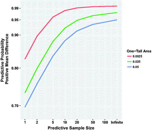As expected, the posterior distribution for difference in means ($M=\infty$) produces a result similar to the hypothesis test (albeit with a very different interpretation) with about 0.025 probability of a negative mean difference. Conversely a repeated experiment with M = 10 per group is predicted to exhibit a negative sample mean difference with probability 0.08 (three times greater). If instead, we consider a single pair of observations, the probability of a negative difference of Y – X is about 0.27; that is, the probability that a control-treated animal (X) is greater than a treated animal (Y). Switching our focus now to positive mean differences, Figure 2 shows the probability of a positive difference for selected tail areas in the original experiment and future sample sizes M. We observe that for small future sample sizes, there remains considerable uncertainty regarding even the sign of the difference in sample means.

Fig. 1 Posterior and conditional predictive distributions for Y - X.

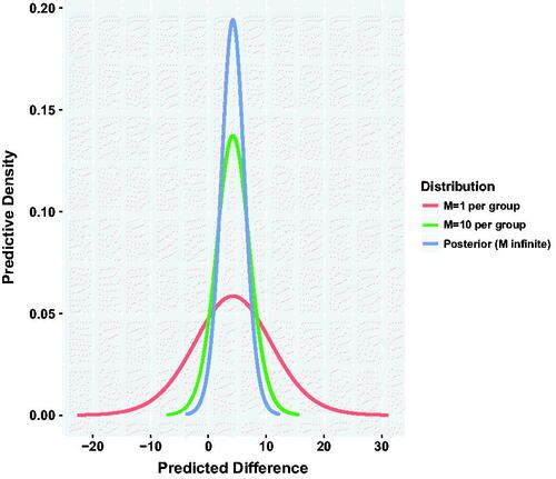
Fig. 2 Predictive probability of a positive mean difference given initial one-sided p-value and sample size N = 10 per group. Curves show the predictive probability of a positive mean difference for different values of predictive sample size and one-tail area (single sided p-value) in the original sample. Thus, an original experiment resulting in p = 0.025 (one tail, green curve), has about 0.92 probability of yielding a positive mean difference in a repeated experiment of M = 10 observations per group.

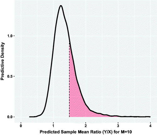
Finally, returning to the wishes of my laboratory collaborators, we would like to predict the probability of a big effect in a future experiment. For the current experiment, the observed treatment fold-change is 1.3 (ratio of treatment means). If we repeat the experiment, what is the probability of at least a 50% treatment-associated increase in sample mean?

Although an analytical solution to this question is not available, a Monte Carlo approximation is easy to program by sampling from scaled-shifted t distributions for each of the two treatment groups. Figure 3 shows the estimated predictive density for a ratio of sample means in a repeated experiment with M = 10 animals per group. We see that the estimated probability of a ratio greater than 1.5 is 0.28. While this value does provide some evidence of a robust treatment effect, it does not suggest that a replication of the experiment will reliably produce the desired result. Note that the predictive approach encourages the use of summaries that are dictated by scientific considerations. We simply summarize the Monte Carlo realizations based on the selected measure.

Fig. 3 Predicted ratio of sample means for a repeated experiment with M = 10 mice per group. The high probability region for the ratio of means ranges from about 0.8 to 2. The red shaded region shows the event that the predicted ratio is greater than 1.5, the minimum important fold change.

5 Conclusion

Most statistical analyses use hypothesis tests about parameters (or occasionally confidence intervals) to form conclusions. They implicitly assume that if the “true parameters” were known, then the problem would be finished (Geisser 1993). Recent proposals, such as simply changing the accepted p-value threshold (Benjamin et al. 2018) to require stronger evidence, do not directly address reproducibility concerns. While a p-value (or Bayes factor) may be useful as a simple numerical summary, it should not be enshrined as the “mother of all statistics” for scientific decision-making.

The point of view expressed here is that parametric modeling can be a useful approximation, and that the values of parameters are important only through their effects on the distribution of future observables. Further, any conclusions or decisions based on these predictions must be judged in the context of the specific problem under study. The predictive inference paradigm encourages scientists (and statisticians) to characterize important results in terms of quantities that can be observed, and to predict the probability of these quantities in future studies.

Moreover, our discipline should move away from context-free decision-making—without a clear sense of losses associated with incorrect decisions. Predictive inference of future observables, given the current data and other related information, can be used as a basis for making coherent decision. This approach brings multiple advantages including

• observed values are easier to interpret than (hypothetical) parameters

• consideration of future observations, whether M = 1 or M = N or $M=\infty$, encourages practitioners to consider how results will be used in future studies and/or in decision-making.

• for settings with finite populations, such as the treatment of rare diseases—inference based on finite sample prediction may be the only appropriate and ethical approach.

Finally, the predictive probability of a scientifically relevant, observable event can be used as a standard for communicating the reliability of the current work, regardless of whether the confirmatory experiment is conducted. If it is conducted, then the future observation can serve to support or detract from the original scientific model. Moreover, predictive inference allows the comparison of competing scientific theories according to the quality of predictions they make, thus leading to better science.

References

- Aitchison, J., and Dunsmore, I. R. (1975), Statistical Prediction Analysis, Cambridge, UK: Cambridge University Press.
- Bedrick, E. J., Christensen, R., and Johnson, W. (1996), “A New Perspective on Priors for Generalized Linear Models,” Journal of the American Statistical Association, 91, 1450–60. DOI: 10.1080/01621459.1996.10476713.
- Benjamin, D. J., Berger, J. O., Johannesson, M., Nosek, B.,…, and Johnson, V. E. (2018), “Redefine Statistical Significance,” Nature Human Behavior, 2, 6–10. DOI: 10.1038/s41562-017-0189-z.
- Briggs, W. (2016), Uncertainty. The Soul of Modeling, Probability and Statistics, Berlin, Germany: Springer International.
- Clarke, B., and Clarke, J. (2012), “Prediction in Several Conventional Contexts,” Statistical Surveys, 6, 1–73. DOI: 10.1214/12-SS100.
- de Finetti, B. (1937), “La prevision: ses lois logiques, ses sources subjectives,” Annals Institute Henri Poincare, 7, 1–68.
- de Finetti, B. (2017), Theory of Probability, vol. IandII, New York: Wiley.
- Geisser, S. (1988), “The Future of Statistics in Retrospect,” in Bayesian Statistics 3, eds. J. M. Bernardo, M. H. DeGroot, D. V. Lindley, and A. F. M. Smith, Oxford, UK: Oxford University Press, pp. 147–158.
- Geisser, S. (1993), Predictive Inference: An Introduction, London: Chapman and Hall/CRC.
- Gelman, A. (2016), “The Problems with p-Values are Not Just with p-Values,” The American Statistician. Supplemental material to the ASA statement on p-values and statistical significance, by Ronald L. Wasserstein & Nicole A. Lazar (2016). The ASA’s Statement on p-Values: Context, Process, and Purpose, The American Statistician, 70, 129–133, [Mismatch] DOI: 10.1080/00031305.2016.1154108.
- Nelder, J. A. (1999), “Statistics for the Millenium,” The Statistician, 48, 257–269. DOI: 10.1111/1467-9884.00187.