Evidence From Marginally Significant t Statistics

ABSTRACT

This article examines the evidence contained in t statistics that are marginally significant in 5% tests. The bases for evaluating evidence are likelihood ratios and integrated likelihood ratios, computed under a variety of assumptions regarding the alternative hypotheses in null hypothesis significance tests. Likelihood ratios and integrated likelihood ratios provide a useful measure of the evidence in favor of competing hypotheses because they can be interpreted as representing the ratio of the probabilities that each hypothesis assigns to observed data. When they are either very large or very small, they suggest that one hypothesis is much better than the other in predicting observed data. If they are close to 1.0, then both hypotheses provide approximately equally valid explanations for observed data. I find that p-values that are close to 0.05 (i.e., that are “marginally significant”) correspond to integrated likelihood ratios that are bounded by approximately 7 in two-sided tests, and by approximately 4 in one-sided tests.

The modest magnitude of integrated likelihood ratios corresponding to p-values close to 0.05 clearly suggests that higher standards of evidence are needed to support claims of novel discoveries and new effects.

KEYWORDS:

• Bayes factor
• Hypothesis test
• Posterior odds
• Prior odds
• Significance level
• Uniformly most powerful Bayesian test
• Weight of evidence

1 Introduction

In a pair of recent articles (Johnson 2013; Benjamin et al. 2017), my coauthors and I recommended that the threshold for declaring “statistical significance” be changed from 0.05 to 0.005. Criticisms of this proposal have focused on comparisons of Type 1 and Type 2 errors, false negative and false positive rates, and other more sophisticated decision-theoretic-based quantities. There is also a persistent misunderstanding regarding the amount of statistical evidence contained in p-values, and many scientists are unwilling to adjust their interpretation of p-values based on more direct measures of evidence. For example, Lakens et al. 2018 states, “given that the marginal likelihood is sensitive to different choices for the models compared, redefining alpha levels as a function of the Bayes factor is undesirable.” Indeed, many nonstatisticians mistakenly interpret p-values as the probability that a null hypothesis is true, and many more are not aware of the relatively arbitrary manner in which the value of 0.05 was chosen to define statistical significance.

In this article, I examine the fundamental question, How much evidence is contained in a t statistic when the p-value is close to 0.05? Ideally, this question would be answered by providing a formula to compute the probability that a null hypothesis is true based on the p-value. That probability is the quantity that scientists are most interested in knowing. Unfortunately, there is no unique mapping from p-values to the probability that a null hypothesis is true, and so this article instead focuses on providing upper bounds on likelihood ratios and integrated likelihood ratios when a p-value of 0.05 is observed. Loosely speaking, a likelihood ratio (LR) represents the ratio of the probability assigned to data under an alternative hypothesis to the probability assigned to data under the null hypothesis. In Bayesian analyses, the LR is directly related to the probability that each hypothesis is true. When the LR is large, the alternative hypothesis provides a better explanation for observed data than the null hypothesis does; when the LR is small, the null provides a better explanation. When the LR is close to 1.0, both hypotheses provide approximately equally valid explanations for observed data. Alternative hypotheses refer to the presence of an effect; the null hypothesis corresponds to no effect. Likelihood ratios can only be computed when all model parameters are completely specified under both hypotheses.

When LR’s cannot be computed, integrated likelihood ratios (ILR’s) can be computed instead. Like LR’s, ILR’s reflect the relative probability assigned to the data by alternative and null hypotheses and thus provide a direct measure of evidence regarding the relative validity of two competing hypotheses. The term integrated likelihood ratio (ILR) is used to describe the ratio of marginal densities obtained by integrating out nuisance parameters that define one or both hypotheses. Integrated likelihoods are one of the two main approaches to handling nuisance parameters, the other being maximization (e.g., profile likelihoods). Integrated likelihoods are used in both frequentist and Bayesian settings, and often have desirable properties not possessed by maximization methods (Kalbfleisch and Sprott 1970; Berger, Liseo, and Wolpert 1990). In Bayesian settings, ILRs are called Bayes factors, but due to the data-dependent nature of the alternative hypotheses considered here, resulting ILRs are not consistent with standard Bayesian practice and so the term Bayes factor has been avoided.

Most of the alternative hypotheses examined in this article have been chosen to bias LR’s and ILR’s in their favor. Similar to earlier analyses in, for example Edwards, Lindman, and Savage (1963), the alternative hypotheses have been chosen to make a p-value of 0.05 look as “significant” as possible. For p-values close to 0.05, I find that LR’s and ILR’s for two-sided tests are less than 7, and LR’s and ILR’s for one-sided tests are less than 4. When ILR’s are calculated as part of a Bayesian analysis, many statisticians feel that values greater than 10 or 20 are required to provide strong evidence in favor of one hypothesis over another (Jeffreys 1961; Kass and Raftery 1995).

2 One-Sided Tests

To begin, consider one-sided tests of a normal mean. Let $X_1,\dots ,X_n$ denote independent random variables with $N(\mu ,{\sigma }^2)$ distributions. For simplicity, suppose that the null and alternative hypotheses are specified as follows:(1) $$H_0:\mu =0,\hspace{1em}{H}_1:\mu \sim N(a,g{\sigma }^2).$$(1)

A normal distribution centered on a with variance g times the observational variance is used to represent the alternative hypothesis. When g = 0, the alternative hypothesis becomes a simple hypothesis, that is, a point mass prior centered on a.¹

The ILR’s considered here for composite hypotheses (i.e., g > 0) are computed under the assumption that the marginal distribution on the variance parameter ${\sigma }^2$ is proportional to $1/{\sigma }^2$. This assumption corresponds to an improper, noninformative prior on the variance parameter and is applied to both the null and alternative hypotheses. It also results in certain numerical (but not philosophical) equivalences between standard frequentist and Bayesian analyses. For example, if a noninformative prior density is also imposed on μ, the Bayesian posterior density for μ is a standard t density. Further discussion of noninformative and improper priors on variance parameters can be found in, for example, Berger and Bernardo (1992).

With these assumptions, the marginal density of the data $\mathbf{X}=\{X_1,\dots ,X_n\}$ under the alternative hypothesis, obtained by integrating out μ and the nuisance parameter ${\sigma }^2$, can be expressed as(2) $$m_1\left(\mathbf{X}\right)=\frac{c {(\mathit{ng}+1)}^{-1/2}}{{\left[1+\frac{t_a^2}{(\mathit{ng}+1)(n-1)}\right]}^{n/2}},$$(2) where(3) $$s^2=\frac{1}{n-1}\sum _{i=1}^n{(X_i-\overline{X})}^2,\hspace{1em}{t}_a=\frac{\overline{X}-a}{s/\sqrt{n}},$$(3) and$$c={\left[\pi (n-1)s^2\right]}^{-n/2}\Gamma \left(\frac{n}{2}\right).$$

The value t_a represents the standard t statistic for testing a hypothesis that $\mu =a$, and s² is the usual sample variance.

The marginal density of the data under the null hypothesis can be obtained by taking a = 0 and g = 0 in (2), yielding(4) $$f(\mathbf{X} ; a=g=0)=\frac{c}{{\left[1+\frac{t_0^2}{(n-1)}\right]}^{n/2}}.$$(4)

The marginal density of the data under the simple alternative hypothesis $\mu =a$ is similarly obtained by taking g = 0 in (2), yielding(5) $$f(\mathbf{X} ; \mu =a,g=0)=\frac{c}{{\left[1+\frac{t_a^2}{(n-1)}\right]}^{n/2}}.$$(5)

For composite alternative hypotheses, it follows that the ILR between the hypotheses specified in (1) can be expressed as(6) $$\text{ILR}=\frac{m_1\left(\mathbf{X}\right)}{f(\mathbf{X} ; a=g=0)}=\frac{{\left[1+\frac{t_0^2}{n-1}\right]}^{n/2}}{\sqrt{\mathit{ng}+1}{\left[1+\frac{t_a^2}{(\mathit{ng}+1)(n-1)}\right]}^{n/2}}.$$(6)

For simple hypotheses, the ILR can be expressed as(7) $$\text{ILR}=\frac{f(\mathbf{X} ; a,g=0)}{f(\mathbf{X} ; a=g=0)}=\frac{{\left[1+\frac{t_0^2}{n-1}\right]}^{n/2}}{{\left[1+\frac{t_a^2}{(n-1)}\right]}^{n/2}}.$$(7)

This equation was obtained by integrating out the variance parameter, ${\sigma }^2$, and setting g = 0 in (2). Alternatively, (7) can be obtained directly by considering the sampling distribution of the t statistic. Under the null hypothesis, t₀ has a standard t density, while under the alternative hypothesis, t_a has a standard t density. Thus, the ILR defined in (7) can also be regarded from the classical perspective as a simple LR.

2.1 Maximum Integrated Likelihood Ratios

From (2), it follows that the maximum probability that can be assigned to the data under the alternative hypothesis is obtained by taking $a=\overline{X}$ and g = 0. For this choice of a and g, the alternative hypothesis becomes a point mass centered on the sample mean, i.e.,(8) $$H_1:\mu =\overline{X}.$$(8)

This assumption maximizes the marginal density of the data under the alternative hypothesis. For this choice of alternative, the ILR simplifies to(9) $${\left[1+\frac{t_0^2}{(n-1)}\right]}^{n/2}.$$(9)

This value represents the maximum value that can be achieved by the ILR for t statistics based on normally distributed data (see Edwards, Lindman, and Savage (1963) for further discussion on maximum likelihood ratios).

In actual scientific practice, sampling variation makes it unlikely that $\overline{X}$ would exactly equal the population mean μ. Nonetheless, Figure 1 depicts the maximum ILR obtained under the alternative hypothesis specified in (8) as a function of the degrees of freedom of the t statistic ν ($=n-1$) when t₀ yields a p-value of 0.05 (i.e., $t_0=T_{0.05}^{\nu }$, where $T_{\alpha }^{\nu }$ represents the $(1-\alpha )$ quantile of a standard t distribution on ν degrees of freedom). Thus, Figure 1 displays the maximum of the ratio between the marginal probabilities assigned to the data under any alternative hypothesis and the null hypothesis when $t_0=T_{0.05}^{\nu }$.

Fig. 1 Maximum integrated likelihood ratio for one-sided t-test yielding p = 0.05.

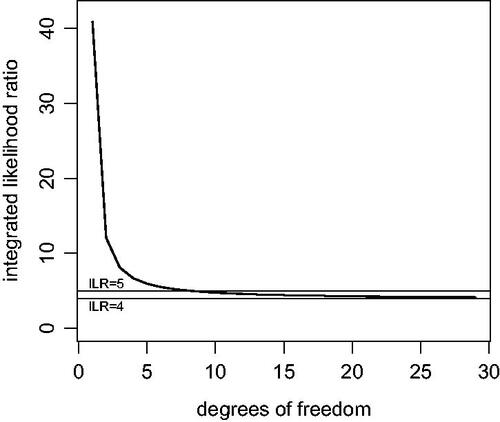
From Figure 1, we see that the ILR is less than 5 whenever there are eight or more degrees of freedom. That is, the data is at least 1/5 as likely under the null hypothesis as it is under any alternative hypothesis regarding the value of μ.

For 1 degree of freedom, the ILR can be as high as 40.9. With 1 degree of freedom (n = 2), this value is obtained when the t statistic ($\sqrt{n}\overline{X}/s$) is 6.31 and the estimated standardized effect size, $\overline{X}/s$, is 4.46. With 5 degrees of freedom, the maximum ILR of 5.95 is obtained when the estimated standardized effect size is 0.82, and for 12 degrees of freedom the maximum ILR of 4.60 is obtained for an estimated standardized effect size of 0.49.

In many studies in the social sciences, the magnitudes of standardized effect sizes (when present) are often smaller than 1.0. For instance, Cohen (1988) classified standardized effect sizes for differences in means as being “small” when near 0.2, “medium” when near 0.5, and “large” when close to 0.8. Sawilowsky (2009) extended these descriptors to “very large” (1.2) and “huge” (2.0) standardized effect sizes. Large effect sizes are often easy to detect, while very small effect sizes may not be of substantive importance. For this reason, hypothesis tests that attempt to detect small to medium effect sizes typically present the greatest challenge and are often of the most substantive interest. If we modify the alternative hypothesis in (8) to restrict μ to be less than 1/2 of an estimated standardized effect size, then a more realistic alternative hypothesis can be expressed as(10) $$H_1:\mu =a=\text{sgn}\left(\overline{X}\right)\min \left(\left|\overline{X}\right|,\frac{s}{2}\right)\hspace{1em}\hspace{1em}\text{and} g=0.$$(10)

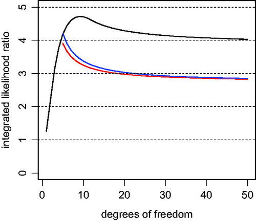
The black curve in Figure 2 depicts the ILR under this alternative hypothesis. It shows that the maximum constrained ILR occurs at 9 degrees of freedom and is 4.71. For estimated standardized effect sizes known to be less than 0.5 (or medium effect sizes in Cohen’s terminology), this figure thus shows that the maximum ILR between the t-statistic under the alternative and null hypotheses is less than 5 whenever p = 0.05.

Fig. 2 ILRs for one-sided tests. The black curve represents the integrated likelihood ratio for one-sided t-tests yielding p = 0.05 under the alternative hypothesis specified in (10). The red curve represents the “average” ILR for a one-sided t-test yielding p = 0.05. The red curve was obtained by replacing the marginal density of the t statistic under the alternative hypothesis by its expectation. The blue curve represents the ILR obtained under the alternative hypothesis corresponding to $a=\overline{X}$ and $g=1/n$ in (1).

2.2 Accounting for Sampling Variation

2.2.1 Classical Approach

For small to medium estimated standardized effect sizes, the ILRs in the previous section assumed that the true population mean μ under the alternative hypothesis exactly equaled the observed sample mean $\overline{X}$. Based on this assumption, the marginal density of the data under the alternative hypothesis was computed from (2) by taking $a=\overline{X}$ and g = 0. Of course, the probability that the sample mean $\overline{X}$ exactly equals the population mean μ is zero.

If, however, the true state of nature was known, then the “true” ILR would be obtained by specifying the alternative hypothesis to be this value. In other words, if the data-generating value of μ was known, we would assume that $a=\mu$ and g = 0 in (1). Under this assumption, the ILR would be assigned the value(11) $$\frac{{\left(1+\frac{t_0^2}{\nu }\right)}^{n/2}}{{\left(1+\frac{t_{\mu }^2}{\nu }\right)}^{n/2}}.$$(11)

Unfortunately, the true value of μ is not known, so the quantity in the denominator cannot be computed.

Because we are conditioning on the event p = 0.05, we know that $\overline{X}=T_{0.05}^{\nu }s/\sqrt{n}$, or, equivalently, that $t_0=T_{0.05}^{\nu }$. Under this condition, the numerator in (11) is a fixed and known quantity. However if we ignore the conditioning on the value of $\overline{X}$, then $t_{\mu }$, evaluated at the true but unknown value of μ, is known to have exactly a t distribution on ν degrees of freedom. This makes it possible to calculate the expected value of(12) $$\frac{1}{{\left[1+\frac{t_{\mu }^2}{\nu }\right]}^{n/2}}.$$(12)

Simple calculations show that this expectation can be expressed as(13) $$E_{\mu }\left[{\left(1+\frac{t_{\mu }^2}{\nu }\right)}^{-n/2}\right]=\frac{\Gamma \left(\frac{n}{2}\right)\Gamma \left(\frac{2n-1}{2}\right)}{\Gamma \left(\frac{n-1}{2}\right)\Gamma \left(n\right)}.$$(13)

Thus, even though we don’t know the true state of nature and the data-generating value of μ, we can compute the expectation of (12) under this value.

It follows that an approximation to the “average ILR” that would be obtained under the true but unknown μ can be expressed as(14) $$\text{average} \text{ILR}\equiv \frac{\Gamma \left(\frac{n}{2}\right)\Gamma \left(\frac{2n-1}{2}\right)}{\Gamma \left(\frac{n-1}{2}\right)\Gamma \left(n\right)}{\left[1+\frac{t_0^2}{\nu }\right]}^{n/2}.$$(14)

Of course, this expression does not equal the expected value of the ILR because the expectation in (13) ignored the condition that $\overline{X}=T_{0.05}^{\nu }s/\sqrt{n}$. Nonetheless, this expression provides an approximation to the average ILR that would be obtained for the “true” alternative hypothesis.

The red curve in Figure 2 depicts the average ILR for $\nu \in (5,50)$ and t statistics that yield p = 0.05. For medium estimated effect sizes (corresponding to more than 5 degrees of freedom), the average ILR is less than 3 when p = 0.05. As before, ILRs greater than 3 can be obtained for $\nu <5$, but these ILRs correspond to comparatively large and easily detectable standardized effect sizes.

2.2.2 Bayesian Approach

A Bayesian approach can also be taken toward evaluating the uncertainty regarding the true value of μ under the alternative hypothesis. For instance, the alternative hypothesis for μ might be assumed to be normally distributed around $\overline{X}$ with variance ${\sigma }^2/n$ (i.e., $a=\overline{X}$ and $g=1/n$). If the variance was known a priori, this assumption would correspond to specifying the alternative hypothesis to be the posterior distribution on μ given the sample mean $\overline{X}$. It leads to the ILRs displayed by the blue curve (Figure 2). This curve produces ILRs that are very similar to the average ILRs obtained in the previous section. Of course, a genuine Bayesian analysis would not be premised on a prior centered on the sample mean, but the similarity between the average ILR and this pseudo-Bayes factor is revealing.

3 Two-Sided Tests

3.1 Bayesian Approach

From a Bayesian perspective, the conduct of a two-sided test suggests that values of μ above and below the null value are possible, which, in turn, suggests that only alternative hypotheses that are symmetric around the null hypothesis should be considered (Berger and Sellke 1987; Sellke, Bayarri, and Berger 2001). Under this constraint, an alternative hypothesis of the following form approximately maximizes the ILR against the null hypothesis (Berger and Sellke 1987, p.116):(15) $$H_1:\mu =\{\begin{array}{cc}\overline{X}& \text{with} \text{probability} \frac{1}{2},\\ -\overline{X}& \text{with} \text{probability} \frac{1}{2}.\end{array}$$(15)

For this alternative hypothesis, the ILR can be expressed as(16) $${\left(1+\frac{t_0^2}{\nu }\right)}^{n/2}\left[\frac{1}{2}+\frac{1}{2}{\left(1+\frac{4t_0^2}{\nu }\right)}^{-n/2}\right],$$(16) where t₀ now refers to $T_{0.025}^{\nu }$.

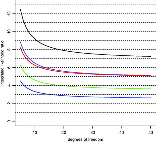
A plot of this ILR against degrees of freedom ν appears as the green curve in Figure 3. This figure suggests that the maximum ILR for marginally significant t statistics under the constraint of a symmetric alternative hypothesis is less than 5 when there are 8 or more degrees of freedom (small to medium estimated effect sizes).

Fig. 3 ILRs for two-sided tests. The black curve depicts the maximum ILR for a two-sided t-test yielding p = 0.05. The alternative hypothesis underlying this curve assumes that $\mu =T_{0.025}^{\nu }s/\sqrt{n}$, the value of the sample mean that produces a two-sided p-value of 0.05. The green curve represents the ILR for a two-sided t-test yielding p = 0.05 obtained by setting $a=\pm \overline{X}$, each with probability one-half, and g = 0. The blue curve was obtained similarly, except that $g=1/n$ to account for variation in the sample mean. The purple curve was obtained by taking $a=\overline{X}$ and $g=1/n$ in (1). The red curve represents the “average” ILR for two-sided t-tests yielding p = 0.05. The marginal likelihood for this curve was obtained by replacing the marginal density of the data under the alternative hypothesis with its expected value at the true value of μ.

As in the case of one-sided tests, the alternative hypotheses used to define the ILRs in the Bayesian test can be revised to account for sampling variability in the value of $\overline{X}$. One approach toward accounting for this variability is to assume a symmetric alternative in which 1/2 mass is assigned to two normal densities centered on $\pm \overline{X}$ and variance ${\sigma }^2/n$. This assumption roughly corresponds to taking one-half of the posterior density centered on $\overline{X}$ and re-centering it on $-\overline{X}$. The integrated likelihood ratio that results from this alternative model is(17) $$\frac{1}{2\sqrt{2}}{\left(1+\frac{t_0^2}{\nu }\right)}^{n/2}\left[1+{\left(1+\frac{2t_0^2}{\nu }\right)}^{-n/2}\right].$$(17)

The blue curve in Figure 3 shows the ILR’s that result from this assumption on the prior distribution. The values in this curve approximately mimic the values of the blue curve in Figure 2, which were based on a similar Bayesian analysis of one-sided tests.

If the symmetry constraint on the alternative hypothesis is removed and the alternative hypothesis is instead defined by taking $a=\overline{X}$ and $g=1/n$, then the ILR can be expressed as(18) $$\frac{1}{\sqrt{2}}{\left(1+\frac{t_0^2}{\nu }\right)}^{n/2}.$$(18)

Values of the ILR under this assumption are represented by the purple curve in Figure 3 and are approximately twice the value of the blue curve.

3.2 Classical Approach

Finally, let us examine ILRs for two-sided t-tests that are significant at the 5% level. The maximum bounds in this case are identical to the bounds that would be obtained in a one-sided t-test that yielded p = 0.025, and are obtained by assuming that the alternative hypothesis specifies that $a=\overline{X}$ and g = 0 in (3). The sample mean is assumed to equal $T_{0.025}^{\nu }s/\sqrt{n}$. The black curve in Figure 3 displays the resulting maximum ILR for 5 or more degrees of freedom, or small to medium estimated standardized effect sizes. Because a two-sided test is performed even though the optimal alternative hypothesis is inherently “one-sided,” the ILRs in this scenario are larger than they were in previous scenarios.

As for one-sided tests, the assumption that the true population mean exactly equals the sample mean is unrealistic. If we account for the sampling variation in the sample mean and instead use the expected value of the t density under the assumption that μ is known (as in (13)), then the average ILR can be approximated by the red curve in Figure 3. The values depicted in this curve are approximately twice the values of the blue curve, which were obtained by placing one-half mass each on $a=\pm \overline{X}$ and $g=1/n$, and are very close to the values in the purple curve obtained by taking $a=\overline{X}$ and $g=1/n$. As noted previously, the factor of 2 in the former arises from the fact that the alternative split the Bayesian posterior distribution into two, re-centering one-half of the posterior distribution on $-\overline{X}$ in order to maintain a symmetric alternative.

The average ILRs in the case of two-sided tests are between 5 and 8 for small to medium estimated standardized effect sizes and p-values near 0.05.

4 Conclusions

Under a variety of assumptions regarding the values of nonzero effects, ILRs in favor of alternative hypotheses are less than 4 for one-sided t tests based on more than 5 degrees of freedom, and are less than 7 for two-sided tests t tests based on more than 7 degrees of freedom. For alternative hypotheses that are constrained to be symmetric around the null hypotheses, ILRs are less than about 5 or 6 for medium estimated standardized effect sizes, and less than about 3 or 4 for small estimated effect sizes in two-sided tests.

This range of ILR values is less conservative than the Bayesian analyses of p-values and Bayes factors presented in Sellke, Bayarri, and Berger (2001), which required alternative hypotheses to be symmetric—and in many cases unimodal—around the null value. That is, Sellke and coauthors estimated ILRs that were even smaller than those exposed here.

The difference in evidence reflected by one-sided and two-sided bounds on ILRs illustrate the importance of properly specifying alternative hypotheses. Indeed, it is quite possible that many journals and regulators implicitly impose significance thresholds of p < 0.025 by requiring that two-sided tests be conducted for alternative hypotheses that are inherently one-sided. Of course, this higher standard for declaring statistical significance is only effective when the sign of an effect is known a priori. It offers no additional protection against HARKing (hypothesizing after results are known; Kerr 1998) when the sign of an effect is not specified before data are analyzed.

In my opinion, the best estimate of the evidence provided by t statistics is provided by the average ILR, which is obtained by replacing the marginal density of data under the alternative hypothesis by its (unconditional) expectation. The expectation of the marginal density of the t statistic under the alternative is free of additional assumptions and represents the exact expectation of a t density at the true value of the population mean μ. It is thus insensitive to prior model choices and other modeling assumptions.

For t statistics based on more than 6 degrees of freedom, the average ILR for two-sided tests is less than 6. For one-sided tests with p-values around 0.05, the average IRL is less than about 3. In other words, the data are, on average, only three or six times more likely under the “true” model than they are under the null hypothesis. Importantly, these values are independent of prior assumptions regarding the value of the population mean under the alternative hypothesis, and apply for all hypothesis tests based on t statistics. They clearly suggest that higher standards of evidence are needed to support claims of novel discoveries and new effects.

Acknowledgments

The author thanks an anonymous associate editor for numerous comments that improved this article.

National Cancer Institute;National Institutes of Health;National Institutes of Health;

Funding

Financial support was provided by NIH award R01 CA158113.

Notes

Notes

1 A simple hypothesis is a hypothesis in which the value of the unknown parameter is completely specified. For composite hypotheses, the value of unknown parameters is only constrained to take values from a specified set, or to be drawn from a specified probability distribution.

References

- Benjamin, D. J., Berger, J. O., Johannesson, M., Nosek, B. A., Wagenmakers, E.–J., Berk, R., Bollen, K. A., Brembs, B., Brown, L., Camerer, C., Cesarini, D., Chambers, C. D., Clyde, M., Cook, T. D., De Boeck, P., Dienes, Z., Dreber, A., Easwaran, K., Efferson, C., Fehr, E., Fidler, F., Field, A. P., Forster, M., George, E. I., Gonzalez, R., Goodman, S., Green, E., Green, D. P., Greenwald, A., Hadfield, J. D., Hedges, L. V., Held, L., Ho, T.–H., Hoijtink, H., Jones, J. H., Hruschka, D. J., Imai, K., Imbens, G., Ioannidis, J. P. A., Jeon, M., Kirchler, M., Laibson, D., List, J., Little, R., Lupia, A., Machery, E., Maxwell, S. E., McCarthy, M., Moore, D., Morgan, S. L., Munafó, M., Nakagawa, S., Nyhan, B., Parker, T. H., Pericchi, L., Perugini, M., Rouder, J., Rousseau, J., Savalei, V., Schönbrodt, F. D., Sellke, T., Sinclair, B., Tingley, D., Van Zandt, T., Vazire, S., Watts, D. J., Winship, C., Wolpert, R. L., Xie, Y., Young, C., Zinman, J., and Johnson, V. E., (2017),“Redefine Statistical Significance,” Nature Human Behaviour, available at https://www.nature.com/articles/s41562-017-0189-z. DOI: 10.1038/s41562-017-0189-z.
- Berger, J. O., and Bernardo, J. M., (1992), “On the Development of Reference Priors” (with discussion), in Bayesian Statistics 4, eds. J.M. Bernardo, J.O. Berger, A.P. Dawid and A.F.M. Smith, New York: Oxford University Press, pp. 35–60.
- Berger, J. O., Liseo, B., and Wolpert, R. L., (1990), “Integrated Likelihood Methods for Eliminating Nuisance Parameters,” Statistical Science, 14, 1–28. DOI: 10.1214/ss/1009211804.
- Berger, J. O., and Sellke, T., (1987), “Testing a Point Null Hypothesis: The Irreconcilability of P Values and Evidence,” Journal of the American Statistical Association, 82, 112–122. DOI: 10.2307/2289131.
- Cohen, J. (1988), Statistical Power Analysis for the Behavioral Sciences, New York: Routledge.
- Edwards, W., Lindman, H., and Savage, L., (1963), “Bayesian Statistical Inference for Psychological Research,” Psychological Review, 70, 193–242. DOI: 10.1037/h0044139.
- Jeffreys, H. (1961), Theory of Probability (3rd ed.) Oxford, UK: Oxford University Press.
- Johnson, V. E. (2013), “Revised Standards for Statistical Evidence,” Proceedings of the National Academy of Sciences, 110, 19313–19317. DOI: 10.1073/pnas.1313476110.
- Kalbfleisch, J., and Sprott, D. A. (1970), “Application of Likelihood Methods to Models Involving Large Numbers of Parameters,” Journal of the Royal Statistical Society, Series B, 32, 175–208. DOI: 10.1111/j.2517-6161.1970.tb00830.x.
- Kass, R., and Raftery, A. E., (1995), “Bayes Factors,” Journal of the American Statistical Association, 90, 773–795. DOI: 10.1080/01621459.1995.10476572.
- Kerr, N. (1998), “HARKing: Hypothesizing after the Results are Known,” Personality and Social Psychology Review, 2, 196–217. DOI: 10.1207/s15327957pspr0203_4.
- Lakens, D., Adolfi, F. G., Albers, C.J., Anvari, F., Apps, M. A. J., Argamon, S. E., Baguley, T., Becker, R.B., Benning, S. D., Bradford, D. E., Buchanan, E. M, Caldwell, A. R., Calster, B. V., Carlsson, R., Chen, S-C., Chung, B., Colling, L. J., Collins, G.S., Crook, Z., Cross, E. S., Daniels, S., Danielsson, H., DeBruine, L., Dunleavy, D.J., Earp, B. D., Feist, M. I., Ferrell, J. D., Field, J. G., Fox, N. W., Friesen, A., Gomes, C, Gonzalez-Marquez, M., Grange, J. A., Grieve, A. P., Guggenberger, R., Grist, J., Harmelen, A., Hasselman, F., Hochard, K. D., Hoffarth, M. R., Holmes, N. P., Ingre, M., Isager, P. M., Isotalus, H. K., Johansson, C., Juszczyk, K., Kenny, D. A., Khalil, A. A, Konat, B., Lao, J., Larsen, E. G., Lodder, G., Lukavsky, J., Madan, C. R., Manheim, D., Martin, S. R., Martin, A. E., Mayo, D. G., McCarthy, R. J., McConway, K., McFarland, C., Nio, A. Q. X., Nilsonne, G., Oliveira, C.L., Xivry, J., Parsons, S., Pfuhl, G., Quinn, K. A., Sakon, J. J., Saribay, S. A, Schneider, I. K., Selvaraju, M., Sjoerds, Z., Smith, S. G., Smits, T., Spies, J. R., Sreekumar, V., Steltenpohl, C. N., Stenhouse, N., Swiatkowski, W., Vadillo, M. A., Van Assen, M., Williams, M. N., Williams, S. E., Williams, D. R., Yarkoni, T., Ziano, I., Zwaan, R. A., (2018), “Justify your Alpha”, Nature Human Behaviour, 2, 168–171. DOI: 10.1038/s41562-018-0311-x.
- Sawilowsky, S. (2009), “New Effect Size Rules of Thumb,” Journal of Modern Applied Statistical Methods, 8, 467–474.
- Sellke, T., Bayarri, M. J., and Berger, J. O., (2001), “Calibration of p Values for Testing Precise Hypotheses,” The American Statistician, 55, 62–71. DOI: 10.1198/000313001300339950.