The False Positive Risk: A Proposal Concerning What to Do About p-Values

Abstract

It is widely acknowledged that the biomedical literature suffers from a surfeit of false positive results. Part of the reason for this is the persistence of the myth that observation of p < 0.05 is sufficient justification to claim that you have made a discovery. It is hopeless to expect users to change their reliance on p-values unless they are offered an alternative way of judging the reliability of their conclusions. If the alternative method is to have a chance of being adopted widely, it will have to be easy to understand and to calculate. One such proposal is based on calculation of false positive risk(FPR). It is suggested that p-values and confidence intervals should continue to be given, but that they should be supplemented by a single additional number that conveys the strength of the evidence better than the p-value. This number could be the minimum FPR (that calculated on the assumption of a prior probability of 0.5, the largest value that can be assumed in the absence of hard prior data). Alternatively one could specify the prior probability that it would be necessary to believe in order to achieve an FPR of, say, 0.05.

KEYWORDS:

• Bayes
• False positive
• False positive report probability
• False positive risk
• FPR
• Likelihood ratio
• Point null
• Positive predictive value

1 Introduction

It is a truth universally acknowledged that some areas of science suffer from a surfeit of false positives.

By a false positive, I mean that you claim that an effect exists when in fact the results could easily have occurred by chance only.

Every false positive that gets published in the peer-reviewed literature provides ammunition for those who oppose science. That has never been more important. There is now strong pressure from within science as well as from those outside it, to improve reliability of the published results.

In the end, the only way to solve the problem of reproducibility is to do more replication and to reduce the incentives that are imposed on scientists to produce unreliable work. The publish-or-perish culture has damaged science, as has the judgment of their work by silly metrics.

In the meantime, improvements in statistical practice can help.

In this article, I am referring to the practice of experimentalists, and to the statistical advice given by journal editors, when they do not have a professional statistician has part of the team. The vast majority of published tests of significance are in this category.

The aim is to answer the following question. If you observe a “significant” p-value after doing a single unbiased experiment, what is the probability that your result is a false positive? In this article, we expand on the proposals made by Colquhoun (2017, 2018) and compare them with some other methods that have been proposed.

2 How Can Statistical Practice by Users and Journals Be Changed?

In the biomedical literature, it is still almost universal to do a test of statistical significance, and if the resulting p-value is less than 0.05 to declare that the result is “statistically significant” and to conclude that the claimed effect is likely to be real, rather than chance. It has been known for many decades that this procedure is unsafe. It can lead to many false positives.

Many users still think that the p-value is the probability that your results are due to chance (Gigerenzer, Krauss, and Vitouch 2004). That, it seems, is what they want to know. But that is not what the p-value tells you.

There can be no doubt that the teaching of statistics to users has failed to improve this practice.

The standard approach in teaching, of stressing the formal definition of a p-value while warning against its misinterpretation, has simply been an abysmal failure. (Sellke, Bayarri and Berger 2001, p. 71)

The ASA statement (Wasserstein and Lazar 2016) gave a cogent critique of p-values. But it failed to come to any conclusions about what should be done. That is why it is unlikely to have much effect on users of statistics. The reason for the lack of recommendations was the inability of statisticians to agree. In the opening words of Kristin Lennox, at a talk she gave at Lawrence Livermore labs,

Today I speak to you of war. A war that has pitted statistician against statistician for nearly 100 years. A mathematical conflict that has recently come to the attention of the “normal” people. (Lennox 2016)

I suggest that the only hope of having the much-needed improvement in statistical practice is to adopt some sort of compromise between frequentist and Bayesian approaches. A good candidate for this is to convert the observed p-value to the false positive risk (FPR). This should appeal to users because the FPR is what most users still think that p-values give them. It is the probability that your result occurred by chance only, a very familiar concept.

There is nothing very new about “recalibrating” p-values, such that they mean what users mistakenly thought they mean. Various ways of doing this have been proposed, notably by Berger and Sellke (1987), Sellke et al. (2001), Goodman (1993, 1999a,b) and by Johnson (2013a,b).

The misinterpretation of p-values is, of course, only one of the widespread misunderstandings of statistics. It is relatively easy to teach users about the hazards of multiple comparisons and the problem of p-hacking. It seems to be much harder to teach what a p-value tells you and what it does not tell you. The abuse of p < 0.05 is still almost universal, at least in the biomedical literature. Journals still give ghastly advice likea level of probability (p) deemed to constitute the threshold for statistical significance should be defined in Methods, and not varied later in Results (by presentation of multiple levels of significance). Thus, ordinarily p < 0.05 should be used throughout a paper to denote statistically significant differences between groups. (Curtis et al. 2014)

Many people have advised culture change. Desirable though that is, such pleading has had very little effect. Others have said that authors should ask a professional statistician. That is obviously desirable too, but there are nowhere near enough statisticians to make that possible, and especially not enough statisticians who are willing to spend time analyzing your data.

The constraints on improvement are as follows.

1. Users will continue to use statistical tests, with the aim of trying to avoid making fools of themselves by publishing false positive results. That is entirely laudable.

2. Most users will not have access to professional statistical advice. There just is not enough of it (in a form that users can understand, and put into practice).

3. The only way to stop people claiming a discovery whenever they observe p < 0.05 is to give them an alternative procedure.

4. Full Bayesian analysis will probably never be adopted as a routine substitute for p-values. It has a place in formal clinical trials that are guided by a professional statistician, but it is too complicated for most users, and experimentalists distrust (rightly, in my view) informative priors. As Valen Johnson said

…subjective Bayesian testing procedures have not been - and will likely never be- generally accepted by the scientific community. (Johnson 2013a,b)

A special case of Bayesian analysis, the false positive risk approach, is simple enough to be widely understood and allows the p-value to be supplemented by a single number that gives a much better idea of the strength of the evidence than a p-value alone.

3 The False Positive Risk Approach

I will consider here only the question of how to avoid false positives when interpreting the result of a single unbiased test of significance. All the other problems of multiple comparisons, inadequate randomization or blinding, p-hacking, etc. can only make matters still worse in real life.

To proceed, we need to define more precisely “the probability that your results are due to chance.” This should be defined as the probability, in the light of the p-value that you observe, you declare that an effect is real, when in fact, it is not. It is the risk of getting a false positive. This quantity has been given various names. For example, it has been called the false positive report rate (FPRP) by Wacholder et al. (2004) though they used the p-less-than approach (see Colquhoun 2017, sec. 3) which is inappropriate for interpretation of single tests. It was called the false discovery rate by Colquhoun (2014, 2016a,b)— this was a foolish choice because it risks confusion with the use of that term in the context of multiple comparison problems (e.g., Benjamini and Hochberg, 1995). A better term is the false positive rate, or, better still, false positive risk. The latter term was recommended by Prof. D. Spiegelhalter (personal communication), because we are talking about interpretation of a single experiment: we are not trying to estimate long-term error rates.

It should be noted that corrections for multiple comparisons aim to correct only the type 1 error rate. The result is essentially a corrected p-value and is, therefore, open to misinterpretation in the same way as any other p-value.

In order to calculate the FPR, it is necessary to invoke Bayes’ theorem. This can be expressed in terms of odds as follows:(1) $${\text{posterior} \text{odds} \text{on} \mathrm{H}}_1=\text{Bayes} \text{factor}\times \text{prior} \text{odds}$$(1)

Or, in symbols,(2) $$\frac{P\left({\mathrm{H}}_1\right|\text{data})}{P\left({\mathrm{H}}_0\right|\text{data})}=\frac{P\left(\text{data}\right|{\mathrm{H}}_1)}{P\left(\text{data}\right|{\mathrm{H}}_0)}\times \frac{P\left({\mathrm{H}}_1\right)}{P\left({\mathrm{H}}_0\right)}$$(2) where H₀ is the null hypothesis and H₁ is the alternative hypothesis.

The bad news is that there are many ways to calculate the Bayes factor (see, e.g., Held and Ott, 2018). The good news is that many of them give similar results, within a factor of 2 or so, so whichever method is used, the conclusions are not likely to differ much in practice. In order to simulate t-tests (e.g., as in Colquhoun 2014), it is necessary to specify an alternative hypothesis,for example, that the true effect size is 1 standard deviation. As we shall see below (Section 5, Figure 1), this does not reduce the generality of the conclusions as much as it might appear at the first sight. Thus, we choose to test$${\mathrm{H}}_0:\theta =0{ \text{against} \mathrm{H}}_1:\theta =\theta 1\ne 0$$

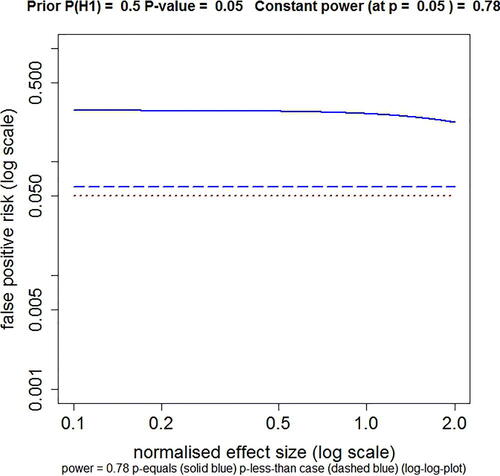
Fig. 1 Plot of FPR against normalized effect size, with power kept constant throughout the curves by varying n. The dashed blue line shows the FPR calculated by the p-less-than method. The solid blue line shows the FPR calculated by the p-equals method. This example is calculated for an observed p-value of 0.05, with power kept constant at 0.78 (power calculated conventionally at p = 0.05), with prior probability P(H₁) = 0.5. The sample size needed to keep the power constant at 0.78 varies from n = 1495 at effect size = 0.1, to n = 5 at effect size = 2.0 (the range of plotted values). The dotted red line marks an FPR of 0.05, the same as the observed p-value. Calculated with Plot-FPR-v-ES-constant-power.R, output file: FPR-vs-ES-const-power.txt (supplementary material).

One advantage of using a simple alternative hypothesis is that the Bayes factor becomes a simple likelihood ratio, and there is no need to postulate a prior distribution, but rather a simple prior probability suffices: $P({\mathrm{H}}_1)=1-P({\mathrm{H}}_0)$ is the probability that there is a real (nonzero) effect size. Thus, Equation (2)(2) $$\frac{P\left({\mathrm{H}}_1\right|\text{data})}{P\left({\mathrm{H}}_0\right|\text{data})}=\frac{P\left(\text{data}\right|{\mathrm{H}}_1)}{P\left(\text{data}\right|{\mathrm{H}}_0)}\times \frac{P\left({\mathrm{H}}_1\right)}{P\left({\mathrm{H}}_0\right)}$$(2) can be written as(3) $$\frac{P\left(H_1\right|\text{data})}{1-P\left(H_1\right|\text{data})}=L_{10}\times \frac{P\left(H_1\right)}{1-P\left(H_1\right)}$$(3) where the likelihood ratio in favor of H₁, relative to H₀, is defined as L₁₀ (following the notation of Held and Ott 2018).(4) $$L_{10}=\frac{P\left(\text{data}\right|H_1)}{P\left(\text{data}\right|H_0)}$$(4)

It has often been argued that the likelihood ratio alone is a better way than a p-value to represent the strength of evidence against the null hypothesis, for example, Goodman (1993, 1999a,b).

It would indeed be a big advance if likelihood ratios were cited, instead of, or as well as, p-values. One problem with this proposal is that very few nonprofessional users of statistics are familiar with the idea of likelihood ratios as evidence. Another problem is that it is hard to judge how big the likelihood ratio must be before it is safe to claim that you have good evidence against the null hypothesis. It seems better to specify the result as an FPR, if only because that is what most users still think, mistakenly, that that is what the p-value tells them (e.g., Gigerenzer, Krauss, and Vitouch 2004). The idea is already familiar to users. That gives it a chance of being adopted. The FPR is$$P\left(H_0\right|\text{data})=1-P(H_1\left|\text{data}\right)$$

so, from Equations (3)(3) $$\frac{P\left(H_1\right|\text{data})}{1-P\left(H_1\right|\text{data})}=L_{10}\times \frac{P\left(H_1\right)}{1-P\left(H_1\right)}$$(3) and (4)(4) $$L_{10}=\frac{P\left(\text{data}\right|H_1)}{P\left(\text{data}\right|H_0)}$$(4) , we get(5) $$\text{FPR}=\frac{1}{1+L_{10}\frac{P\left(H_1\right)}{1-P\left(H_1\right)}}.$$(5)

Thus, in the case where the prior probability, P(H₁) = 0.5, the FPR is seen to be just another way of expressing the likelihood ratio:$$\text{FPR}=\frac{1}{1+L_{10}}.$$

Notice that we have chosen to write the likelihood ratio as the odds on H₁. The bigger the value, the more probable is the data given H₁, relative to H₀. Often the likelihood ratio is written the other way up, as L₀₁ = 1/L₁₀, so large values favor H₀. References to minimum values of L₀₁—the smallest evidence for H₀—are, therefore, equivalent to maximum values for L₁₀, the greatest evidence for there being a real nonzero effect that is provided by the data.

In the case of a simple alternative hypothesis, the likelihood ratio can be calculated in two different ways: the p-equals approach or the p-less-than approach (e.g. Goodman 1993, 1999b, and sec. 3 in Colquhoun, 2017). Once the experiment is done, the p-value that it produces is part of the observations. We are interested only in the particular p-value that was observed, not in smaller p-values that were not observed. Since the aim of this work is to interpret a single p-value from a single experiment (rather than trying to estimate the long term error rate), the p-equals method is the appropriate way to calculate likelihood ratios.

For small samples, for which a t-test is appropriate, the likelihood ratio can be calculated as a ratio of probability densities (see the appendix). The effect of sample size on FPR was investigated by Colquhoun (2017).

Bayes’ theorem requires that we specify a prior probability and in the vast majority of cases, we do not know what it is. But I don’t think that that means we have to give up on the FPR.

There are two ways to circumvent the inconvenient fact that we cannot give a value for the prior probability that there’s a real effect. One is to assume that the prior probability of a real effect, P(H₁), is 0.5, that is, that there is a 50:50 chance of there being a real effect before the experiment was done. The other way is to calculate the prior that you would need to believe in order to achieve an FPR of, say 5%. This so-called reverse Bayes approach was mentioned by Good (1950) and has been used, for example, by Carlin and Louis (1996), Matthews (2001, 2018), Held (2003) and Colquhoun (2017, 2018). In both cases, it would be up to you to persuade your readers and journal editors that the value of the prior probability is reasonable. Inductive inference inevitably has an element of subjectivity (Colquhoun 2016).

The proposal to specify the FPR is likely to be more acceptable to users than most because it uses concepts which are familiar to most users. It starts by calculating p-values and uses the familiar point null hypothesis. The idea of prior probability can be explained via diagnostic screening tests and the results can be explained to users by simulation of tests (e.g., Colquhoun 2014).

Exact calculations can be done using R programs (Colquhoun 2017), or with a web calculator (Colquhoun and Longstaff 2017). The variables involved are the observed p-value, the FPR, and the prior probability that there is a real effect. If any two of these are specified, the third can be calculated. The calculations give the same FPR if the number of observations and the normalized effect size are adjusted to keep the power constant (Figure 1 and Colquhoun 2017), so when doing the calculations these should be chosen to match the power of your experiment: see Section 5.

4 The Point Null

Some people do not like the assumption of a point null that is made in this proposed approach to calculating the FPR, but it seems natural to users who wish to know how likely their observations would be if there were really no effect (i.e., if the point null were true). It is often claimed that the null is never exactly true. This is not necessarily so (just give identical treatments to both groups). But more importantly, it does not matter. We are not saying that the effect size is exactly zero: that would obviously be impossible. We are looking at the likelihood ratio, that is, at the probability of the data if the true effect size were not zero relative to the probability of the data if the effect size were zero. If the latter probability is bigger than the former then clearly we cannot be sure that there is anything but chance at work. This does not mean that we are saying that the effect size is exactly zero. From the point of view of the experimenter, testing the point null makes total sense. In any case, it makes little difference if the null hypothesis is a narrow band centered on zero (Berger and Delampady 1987).

5 The Simple Alternative Hypothesis

It was stated above that the need to specify a fixed alternative hypothesis is not as restrictive as it seems at first. This is the case because FPR is essentially independent of the effect size if the power of the experiment is constant. This is illustrated in Figure 1, which shows the result of plotting FPR against the true normalized effect size. In this graph, the power is kept constant by changing the sample size, n, for each point. The power is calculated in the standard way, for the normalized effect size and p = 0.05. When the FPR is calculated by the p-less-than method, it is exactly independent of the effect size. When the FPR is calculated by the p-equals method, as is appropriate for our problem, the FPR is essentially independent of effect size up to an effect size of about 1 (standard deviation) and declines only slightly for larger effects. This is the basis for the recommendation that the inputs for the calculator should match the power of the actual experiment.

6 The Jeffreys–Lindley “Paradox”

It may be surprising, at first sight, that the FPR approaches 100% as the sample size is increased when it is calculated by the p-equals method, whereas the FPR decreases monotonically with sample size when it is calculated by the p-less-than method. The former case is illustrated in Figure 2. As sample size increases, the evidence in favor of the null hypothesis declines at first but then increases.

Fig. 2 FPR plotted against n, the number of observations per group for a two independent sample t-test, with normalized true effect size of 1 standard deviation. The FPR is calculated by the p-equals method, with a prior probability P(H₁) = 0.5 (Equation A6(A6) $$\text{FPR}=\frac{1}{1+L_{10}\frac{P\left({\mathrm{H}}_1\right)}{1-P\left({\mathrm{H}}_1\right)}}$$(A6) ). Log–log plot. Calculations for four different observed p-values, from top to bottom these are: p = 0.05 (blue), p = 0.01 (green), p = 0.001 (red), p = 0.0001 (orange). The power of the tests varies throughout the curves. For example, for the p = 0.05 curve, the power is 0.22 for n = 4 and power is 0.9999 for n = 64 (the extremes of the plotted range). The minimum FPR (marked with gray-dashed lines) is 0.206 at n = 8. This may be compared with the FPR of 0.27 at n = 16, at which point the power is 0.78 (as in Colquhoun, (2014), (2017)). Values for other curves are given in the print file for these plots (Calculated with Plot-FPR-vs-n.R. Output file: Plot-FPR-vs-n.txt. supplementary material).

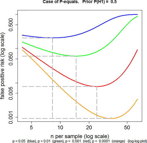
This phenomenon is an example of the Jeffreys–Lindley “paradox” (Lindley 1957; Bartlett 1957).

It can be explained intuitively as follows.

It is convenient to use the web calculator at http://fpr-calc.ucl.ac.uk/. The third radio button shows that for p = 0.05, and normalized effect size of 1, a sample of 16 observations in each group gives a power of 0.78. That is usually considered to be a well-powered experiment. Many published experiments have much lower power. For an observed p-value of 0.05, the FPR for n = 16 and a prior of 0.5 is 27% when calculated by the p-equals method. This is one way of looking at the weakness of the evidence against the null hypothesis that is provided by observing p = 0.05 in a single well-powered experiment. Another way is to note that the likelihood ratio in favor of there being a real effect (null hypothesis being untrue) is only about 3 to 1 (2.76, see Colquhoun 2017, sec. 5.1). This is much less than the odds of 19:1 that are often wrongly inferred from the observed p = 0.05.

Now to explain the apparent paradox. If the sample size is increased from 16 to 64, keeping everything else the same, the FPR increases from 0.78 (at n = 16) to 0.996 (at n = 64) when calculated by the p-equals method, that is, observation of p = 0.05 when n = 64 provides strong evidence for the null hypothesis. But notice that this sample size corresponds to a power of 0.9999, far higher than is ever achieved in practice. The reason for the increased FPR with n = 64 can be understood by looking at the corresponding likelihood ratios. If the calculation for n = 64 is done by the p-less-than method, the likelihood ratio is 20.0—quite high because most p-values will be less than 0.05 in this situation. But the likelihood ratio found by the p-equals method has fallen from 2.76 for n = 16, to 0.0045 for n = 64. In words, the observation (of p = 0.05) would be 222 times as likely (1/0.0045) if the null hypothesis were true than it would be if the null hypothesis were false. So observing p = 0.05 provides strong evidence for the null hypothesis in this case. The reason for this is that with n = 64 it is very unlikely that a p-value as big as 0.05 would be observed: 99.99% of p-values are less than 0.05 (that is the power), and 98.7% of p-values are less than 0.001 (found using the R script two_sample-simulation-+LR.R: supplementary material). With a power of 0.9999, it would be very suspicious indeed to observe a p-value as big as 0.05.

The resolution of this problem is given in Appendix A4 of Colquhoun (2017), and in the Notes tab of the calculator. Make sure that the power matches that of your experiment. If you use a silly power, you will get a silly answer.

7 Some Alternative Proposals

The suggestion made here is one of several that have been made with the aim of expressing evidence in ways that do not suffer from the same problems as p-values. They are all based on normal distributions apart from the present proposal (Colquhoun 2014, 2017) which is based on Student’s t distribution so that its results are appropriate for the small samples that typify most lab work.

1. Many authors have proposed replacement of null hypothesis testing with full Bayesian analysis. These have their place in, for example, large clinical trials with a professional statistical advisor. But they are unlikely to replace the p-value in routine use for two reasons. One is that experimenters will probably never trust the use of informative prior distributions that are not based on hard evidence. The other is that the necessity to test a range of priors makes statement of the results too lengthy and cumbersome for routine use in papers that often cite many p-values.

2. Senn (2015) has produced an example in which the FPR is close to the p-value. This uses a smooth prior distribution, rather than the lumped prior used here, and has, so far, been demonstrated only for one-sided tests. This result differs from the results obtained by simulation of repeated t-tests (Colquhoun 2014) and is in contrast with the general view that the FPR is bigger, often much bigger, than the p-value.

3. It has been proposed, as an interim way to reduce the risk of false positives, that the threshold for significance should be reduced from 0.05 to 0.005 (Benjamin et al. 2017). This proposal has the huge disadvantage that it perpetuates the dichotomization into “significant” and “nonsignificant.” And even p = 0.005 is not safe for implausible hypotheses (see Colquhoun 2017, sec. 9 and Table 1). The value of p = 0.005 proposed by Benjamin et al. (2017) would, in order to achieve an FPR of 5%, require a prior probability of real effect of about P(H₁) = 0.4 (from the web calculator, with power = 0.78). It is, therefore, safe only for plausible hypotheses. If the prior probability were only P(H₁) = 0.1, the FPR with p = 0.005 would be 24% (from the web calculator: Colquhoun and Longstaff 2017). It would still be unacceptably high even with p = 0.005. In order to reduce the FPR to 5% with a prior probability of P(H₁) = 0.1, we would need to observe p = 0.00045. This conclusion differs from that of Benjamin et al. (2017) who say that the p = 0.005 threshold, with prior = 0.1, would reduce the FPR to 5% (rather than 24%). This is because their calculation is based on the p-less-than interpretation which, in my opinion, is not the correct way to look at the problem (see Colquhoun 2017, sec. 3).

4. Matthews (2018) proposed a more sophisticated version of the reverse Bayesian proposal made here. He shows that, in the case where there is no objective prior information, the observation of p = 0.013 implies 95% credibility, in the Bayesian sense (though Matthews does not suggest that this should be used as a revised threshold value). This can be compared with the approach of Colquhoun (2017) which says that when you observe p = 0.013 that you would need a prior probability of there being a real effect of 0.61 to achieve an FPR of 0.05 (with the default inputs, power = 0.78). Or alternatively (using the third radio button on the web calculator), that the FPR is 7.7% for a prior of 0.5.

Table 1 Calculations done with web calculator http://fpr-calc.ucl.ac.uk/, or with R scripts (see the appendix).

			Minimum FPR (mFPR)			False positive risk, FPR with
			prior = 0.5			prior = 0.1
Observed	Likelihood	Prior for	Colquhoun	Sellke–Berger	Goodman	Colquhoun	Sellke–Berger	Goodman
p-value	ratio: (H1/H0)	FPR = 0.05	value	value	value	value	value	value
0.05	2.8	0.87	0.27	0.29	0.227	0.76	0.79	0.725
0.025	6.1	0.76	0.14	0.20	0.140	0.60	0.69	0.593
0.01	15	0.55	0.061	0.11	0.068	0.37	0.53	0.395
0.005	29	0.40	0.034	0.067	0.037	0.24	0.39	0.259
0.001	100	0.16	0.0099	0.018	0.0088	0.082	0.14	0.074

NOTES: Column 1: The observed p-value.

Column 2: Likelihood ratios (likelihood for there being a real effect divided by likelihood of null hypothesis). Calculated for a well-powered (0.78) experiment, as in Equation (A5)(A5) $$L_{10}=\frac{L\left({\mathrm{H}}_1\right)}{L\left({\mathrm{H}}_0\right)}=\frac{\text{Prob}\left(\text{data}\right|H_1)}{\text{Prob}\left(\text{data}\right|H_0)}=\frac{y_1}{2y_0}$$(A5) and Colquhoun (2017).

Column 3: The prior probability of there being a real effect, P(H₁), that it would be necessary to postulate in order to achieve an FPR (FPR) of 5%. Calculated for a well-powered (0.78) experiment as in Equation (A7)(A7) $$P\left({\mathrm{H}}_1\right)=\frac{(1-\text{FPR})}{(1-\text{FPR}+L_{10}\text{FPR})}$$(A7) . (The reverse Bayes approach: Colquhoun (2017)).

Columns 4–6: The minimum FPR, that is, the FPR that corresponds to prior probability of P(H₁) = 0.5, calculated by three methods, Colquhoun value (calculated for a well-powered (0.78) experiment as in Equations (A5)(A5) $$L_{10}=\frac{L\left({\mathrm{H}}_1\right)}{L\left({\mathrm{H}}_0\right)}=\frac{\text{Prob}\left(\text{data}\right|H_1)}{\text{Prob}\left(\text{data}\right|H_0)}=\frac{y_1}{2y_0}$$(A5) and (A6)(A6) $$\text{FPR}=\frac{1}{1+L_{10}\frac{P\left({\mathrm{H}}_1\right)}{1-P\left({\mathrm{H}}_1\right)}}$$(A6) and Colquhoun (2017). Sellke–Berger value: calculated as in Equations (A8)(A8) $$L_{10}=\frac{1}{-\mathit{ep}\hspace{0.17em}\text{log}\hspace{0.17em}\left(p\right)}$$(A8) and (A6)(A6) $$\text{FPR}=\frac{1}{1+L_{10}\frac{P\left({\mathrm{H}}_1\right)}{1-P\left({\mathrm{H}}_1\right)}}$$(A6) . Goodman value, calculated as in Equations (A9)(A9) $$L_{10}=\frac{1}{2\hspace{0.17em}\text{exp}\hspace{0.17em}(-z^2/2)}$$(A9) and (A6)(A6) $$\text{FPR}=\frac{1}{1+L_{10}\frac{P\left({\mathrm{H}}_1\right)}{1-P\left({\mathrm{H}}_1\right)}}$$(A6) .

Columns 7–9. As columns 4–6, but for an implausible hypothesis with prior probability, P(H₁) = 0.1.

In practice there is not much difference between a prior of 0.61 and 0.5 (or between an FPR of 7.7% and 5%), and to that extent both approaches give similar answers. But my approach would give a much bigger FPR for implausible hypotheses (those with priors, P(H₁), less than 0.5), but Matthews (2018) would deal with implausible hypotheses in a different way.

1. Bayesian approaches which use a prior distribution that is most likely to reject the null hypothesis. These include Berger and Sellke (1987) and Sellke et al. (2001)—(see the appendix), and V. Johnson’s uniformly most powerful Bayesian tests (Johnson 2013a,b), For example, if we observe p = 0.05, Berger et al. find an FPR of 22%–29% and Johnson finds 17%–25%. These are comparable with the FPR of 27% found here for a well-powered study with a prior probability of 0.5.

2. Goodman (1999b) has given an expression for calculating the maximum likelihood ratio in favor of H₁ in the case where samples are large enough that the normal distribution, rather than Student’s t, is appropriate (see, Equation A9(A9) $$L_{10}=\frac{1}{2\hspace{0.17em}\text{exp}\hspace{0.17em}(-z^2/2)}$$(A9) ).

Three of these approaches are compared in Figure 3 and in Table 1.

Fig. 3 Comparison of three approaches to calculation of FPR in the case of a simple alternative hypothesis. Solid blue line: the p-equals method for t-tests described in Colquhoun (2017), and Equations (A5)(A5) $$L_{10}=\frac{L\left({\mathrm{H}}_1\right)}{L\left({\mathrm{H}}_0\right)}=\frac{\text{Prob}\left(\text{data}\right|H_1)}{\text{Prob}\left(\text{data}\right|H_0)}=\frac{y_1}{2y_0}$$(A5) and (A6)(A6) $$\text{FPR}=\frac{1}{1+L_{10}\frac{P\left({\mathrm{H}}_1\right)}{1-P\left({\mathrm{H}}_1\right)}}$$(A6) . Dashed blue line: the Sellke–Berger approach, using Equations (A8)(A8) $$L_{10}=\frac{1}{-\mathit{ep}\hspace{0.17em}\text{log}\hspace{0.17em}\left(p\right)}$$(A8) and (A6)(A6) $$\text{FPR}=\frac{1}{1+L_{10}\frac{P\left({\mathrm{H}}_1\right)}{1-P\left({\mathrm{H}}_1\right)}}$$(A6) . Dotted blue line: the Goodman approach, calculated using Equations (A9)(A9) $$L_{10}=\frac{1}{2\hspace{0.17em}\text{exp}\hspace{0.17em}(-z^2/2)}$$(A9) and (A6)(A6) $$\text{FPR}=\frac{1}{1+L_{10}\frac{P\left({\mathrm{H}}_1\right)}{1-P\left({\mathrm{H}}_1\right)}}$$(A6) . Dotted red line is where points would lie if FPR was equal to the p-value. This example is calculated for n = 16, normalized effect size = 1 and prior probability P(H₁) = 0.5. Log–log plot. Calculated with Plot-FPR-vs-Pval + Sellke-Goodman.R (supplementary material).

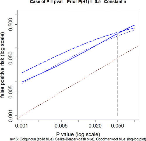
Figure 3 shows the FPR plotted against the observed p-value. The solid blue line is calculated as in Colquhoun (2017), for a well-powered experiment (n = 16, normalized effect size = 1 SD), using the p-equals method, and prior probability P(H₁) = 0.5 (Equations A5(A5) $$L_{10}=\frac{L\left({\mathrm{H}}_1\right)}{L\left({\mathrm{H}}_0\right)}=\frac{\text{Prob}\left(\text{data}\right|H_1)}{\text{Prob}\left(\text{data}\right|H_0)}=\frac{y_1}{2y_0}$$(A5) and A6(A6) $$\text{FPR}=\frac{1}{1+L_{10}\frac{P\left({\mathrm{H}}_1\right)}{1-P\left({\mathrm{H}}_1\right)}}$$(A6) ). The dashed blue line shows the FPR calculated by the Sellke–Berger approach (Equations A8(A8) $$L_{10}=\frac{1}{-\mathit{ep}\hspace{0.17em}\text{log}\hspace{0.17em}\left(p\right)}$$(A8) and A6(A6) $$\text{FPR}=\frac{1}{1+L_{10}\frac{P\left({\mathrm{H}}_1\right)}{1-P\left({\mathrm{H}}_1\right)}}$$(A6) ), and the dotted blue line is calculated by the Goodman approach (Equations A9(A9) $$L_{10}=\frac{1}{2\hspace{0.17em}\text{exp}\hspace{0.17em}(-z^2/2)}$$(A9) and A6(A6) $$\text{FPR}=\frac{1}{1+L_{10}\frac{P\left({\mathrm{H}}_1\right)}{1-P\left({\mathrm{H}}_1\right)}}$$(A6) ). In all cases, the FPR is a great deal bigger than the p-value (equality is indicated by the dotted red line). The Goodman approach agrees quite well with that of Colquhoun (2017) for observed p-values below 0.05, the range of interest. The Sellke–Berger approach gives larger FPR s over this range, but does not differ enough that the conclusions would differ much in practice.

Table 1 shows values calculated for five different observed p-values, shown in column 1. The second column shows the corresponding likelihood ratios, calculated as in Colquhoun (2017), and Equation (A5)(A5) $$L_{10}=\frac{L\left({\mathrm{H}}_1\right)}{L\left({\mathrm{H}}_0\right)}=\frac{\text{Prob}\left(\text{data}\right|H_1)}{\text{Prob}\left(\text{data}\right|H_0)}=\frac{y_1}{2y_0}$$(A5) . These are calculated from the known effect size and standard deviation, but calculations based on the observed effect size and sample standard deviation are similar, especially for p-values below 0.01 (see Colquhoun 2017, sec. 5.1). For example, the last row of Table 1 shows that if you observed p = 0.001, the likelihood ratio in favor of H₁ would be 100, which would normally be regarded as very strong evidence against the null hypothesis. However, this is not necessarily true. If the prior probability P(H₁) were only 0.1, then Table 1 shows that the FPR would be 0.08, still bigger that the conventional 5% value. In this case, you would need to observe p = 0.00045 in order to achieve an FPR of 0.05 (e.g., using radio button 2 on the calculator at http://fpr-calc.ucl.ac.uk/)

The third column of Table 1 shows the result of the reverse Bayesian approach, proposed by Matthews (2001) and by Colquhoun (2017), calculated with Equation (A7)(A7) $$P\left({\mathrm{H}}_1\right)=\frac{(1-\text{FPR})}{(1-\text{FPR}+L_{10}\text{FPR})}$$(A7) . If you observed p = 0.05, then in order to achieve an FPR = 0.05 you would need to persuade your readers that it was reasonable to assume a very high prior probability, P(H₁) = 0.87, that the observed effect was not merely chance. It is unlikely that anyone would believe that in the absence of hard evidence. If you observed p = 0.005 (penultimate row of Table 1) the prior needed to achieve FPR = 0.05 would be 0.4, so you would be safe if the hypothesis was reasonably plausible.

The remaining columns of Table 1 show the FPR s that correspond to each of the p-values in column 1. They are calculated as described in the appendix, for prior probabilities, P(H₁) = 0.5 and for P(H₁) = 0.1.

It is gratifying that all three methods of calculating the FPR give results that are close enough to each other that much the same conclusions would be drawn in practice. All of them suggest that if you observe p = 0.05 in an unbiased, well-powered experiment, and you claim a discovery on that basis, you are likely to be wrong at least 20–30% of the time, and over 70% of the time if the hypothesis is a priori implausible: (P(H₁) = 0.1).

8 Real-Life Examples

Example 1

The data used by Student (1908).

The results in Table 2 are observations made by Cushny and Peebles (1905) on the sleep-inducing properties of (–)-hyoscyamine (drug A) and (–)-hyoscine (drug B). These data were used W. S. Gosset as an example to illustrate the use of his t-test, in the paper in which the test was introduced (Student, 1908). The conventional t-test for two independent samples is done as follows (more detail in Colquhoun 1971, sec. 9.4).

Number per sample: n_A = 10, n_B = 10.

Mean response: drug A: + 0.75; drug B + 2.33.

Standard deviations: drug A $s(y_A)=1.78901$; drug B $s(y_B)=2.002249$.

Effect size (difference between means): E = 2.33 – 0.75 = 1.58.

We wish to test whether drug B is really better than A or whether the results could have plausibly arisen if the null hypothesis (true difference is zero) were true.

The pooled estimate of the error within groups is$$s\left(y\right)=\sqrt{\frac{(n_A-1)s{\left(y_A\right)}^2+(n_B-1)s{\left(y_B\right)}^2}{(n_A-1)+(n_B-1)}}=1.899$$

Normalized effect size $=E/s(y)=0.83218$.

Standard deviation of effect size $s_E=\sqrt{\frac{s{(y)}^2}{n_A}+\frac{s{(y)}^2}{n_B}}=0.84909$.

Degrees of freedom: $(n_A-1)+(n_B-1)=18$.

Student’s $t: t_{18}=\frac{E}{s_E}=1.8608$.

P = 0.07918

The p-value exceeds 0.05 so the difference between means would conventionally be described as “non-significant.” A very similar p-value (0.08) is obtained from the same data by the randomization test (Colquhoun 1971, sec. 9.2); or, in more detail, in Colquhoun (2015), in which all 184,756 ways of selecting 10 observations from 20 are plotted.

This conventional p-value result can now be compared with the FPR result. This can be done most conveniently by use of the web calculator (http://fpr-calc.ucl.ac.uk/). The inputs for the calculator are the p-value (0.07918), the normalized effect size (0.83218), and the sample size (n = 10). If the prior probability of a real effect were 0.5, then the minimum FPR (mFPR) would be 0.28, a lot bigger than the p-value (and it would be bigger still if the hypothesis were thought to be implausible, that is, if its prior probability were less than 0.5). Another way to express the uncertainty is to note that in order to make the FPR 5%, we would have to postulate a prior probability of there being a real effect, P(H₁) = 0.88. Without strong prior evidence, the existence of a real effect is very doubtful. A third way to put the result is to say that the likelihood ratio is only 2.54 so the evidence of the experiment makes the existence of a real effect only 2.54 times as likely as it was before the experiment.

The calculator shows also that the power of this study, calculated for p = 0.05 using the observed response size and standard deviation is only 0.42.

Table 2 Response in hours extra sleep (compared with controls) induced by (–)-hyoscyamine (A) and (–)-hyoscine (B). From Cushny and Peebles (1905).

Drug A yA	Drug B yB
+0.7	+1.9
−1.6	+0.8
−0.2	+1.1
−1.2	+0.1
−0.1	−0.1
+3.4	+4.4
+3.7	+5.5
−0.8	+1.6
0.0	+4.6
+2.0	+3.4

Example 2 A

study of transcranial electromagnetic stimulation.

A study of transcranial electromagnetic stimulation (TMS), published in Science, concluded that TMS “improved associative memory performance,” p = 0.043 (Wang et al. 2014).

The authors of this article said only “The increase in performance for baseline to Post-Tx was greater for stimulation than for sham [T₍₁₅₎ = 2.21, p = 0.043].” The mean raw scores (numbers of words correctly recalled to associated face cues) are given in their Table S2 in the supplementary material. The calculations use the change in score between baseline and post-treatment. The effect size is the difference in this quantity between stimulation and sham. From Table S2, the effect size is 1.88 with standard deviation 1.70 (n = 8). The normalized effect size is, therefore, 1.88/1.70 = 1.10, and the post hoc power is 0.54. Rather than saying only “p = 0.043,” better ways to express the result of this experiment would be as follows (found from the web calculator, radio buttons 3, 1, and 2, respectively). In all cases, the effect size and its confidence interval should be given in the text, not relegated to the supplementary material.

The increase in memory performance was 1.88 ± 0.85 (stand deviation of the mean, i.e., standard error) with confidence interval 0.055–3.7 (extra words recalled on a baseline of about 10). Thus, p = 0.043.

This should be supplemented as follows:

1. The observation of p = 0.043 implies a minimum FPR (that for prior probability, P(H₁) = 0.5), of at least 18%. This is the probability that the results occurred by chance only, so the result is no more than suggestive.

or

1. The increase in performance gave p = 0.043. In order to reduce the FPR to 0.05, it would be necessary to assume that we were almost certain (prior probability, P(H₁) = 0.81) that there was a real effect before the experiment was done. There is no independent evidence for this assumption so the result is no more than suggestive.

or

1. The increase in performance gave p = 0.043. In order to reduce the minimum FPR to 0.05, it would have been necessary to observe p = 0.0043, so the result is no more than suggestive.

Of these options, the first is probably the best because it is the shortest, and because it avoids the suggestion that FPR = 0.05 is being suggested as a new “bright line,” in place of p = 0.05.

9 Conclusions

In my proposal, the terms “significant” and “nonsignificant” would not be used at all. This change has been suggested by many other people, but these suggestions have had little or no effect on practice. A p-value and confidence interval would still be stated but they would be supplemented by a single extra number that gives a better measure of the strength of the evidence than is provided by the p-value.

1. This number could be the minimum FPR, that is, that calculated on the basis that the prior probability of a real effect is 0.5 (the largest value that it is reasonable to assume without hard evidence for a higher value: see Colquhoun, 2017, fig. 3). This has the advantage that it is easy to understand. It has the disadvantage that it is safe only for plausible hypotheses. Nonetheless, it would be a lot better than giving only the p-value and confidence interval.

2. Or the additional number could be the prior probability that you would need to believe in order to achieve an FPR of, say, 0.05. This has the disadvantage that most users are unfamiliar with the idea of prior probabilities, which are, in most cases subjective probabilities. It also runs the risk that FPR = 0.05 will become a new “threshold,” in place of p = 0.05.

Examples of improved ways to express the strength of the evidence are given above, at the end of Section 8.

I appreciate that my proposal is only one of many ways to look at the problem of false positives. Other approaches can give different answers. But it has the virtue of being simple to understand and simple to calculate. Therefore it has a chance of being adopted widely.

All the results in this article have been derived in the context of p-values found from t-tests of the difference between means of two independent samples. The question of the extent to which they apply to p-values found in other ways remains to be investigated. Since the logical flaw in the use of p-values as a measure of the strength of evidence is the same however they are derived, it seems likely that the FPRs will be similar in other situations.

Of course any attempt to reduce the number of false positives will necessarily increase the number of false negatives. In practice, decisions must depend on the relative costs (in reputation, or in money, or both) that are incurred by wrongly claiming a real effect when there is none, and by failing to detect a real effect when there is one.

Supplementary Materials

R scripts (and output files) used for calculations and plots are provided as online supplementary materials.

Acknowledgments

I am especially grateful to the following people: Dr Leonhard Held Epidemiology, Biostatistics and Prevention Institute, University of Zurich, CH-8001 Zurich, for helpful discussions; Dr R.A.J. Matthews for helpful discussions about his paper (Matthews 2018); Prof. Stephen Senn (Competence Center in Methodology and Statistics, CRP-Santé, Luxembourg); and Prof. D. Spiegelhalter for reading an earlier version of Colquhoun (2017) and suggesting the term “false positive risk.”

Appendix

In this appendix, we give details of three methods of calculating the likelihood ratio, hence the FPR, for tests of a point null hypothesis against a simple alternative.

Appendix A1

The p-equals approach as used by Colquhoun (2017)

The critical value of the t statistic is calculated from the observed p-value as(A1) $$t_{\mathit{crit}}=\mathit{qt}\left(1-\frac{p}{2},\mathit{df},\mathit{ncp}=0\right)$$(A1) where qt() is the inverse cumulative distribution of Student’s t statistic (the notation is as in R). The arguments are the observed p-value, p, the number of degrees of freedom, df, and the noncentrality parameter, ncp (zero under the null hypothesis)

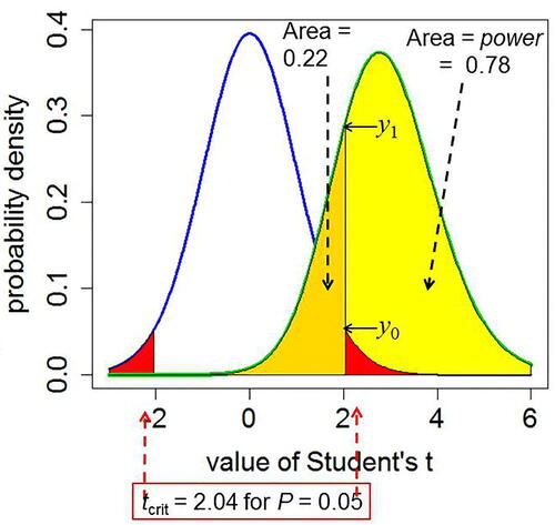
Numerical values given in this section all refer to the example shown in Figure A1 (reproduced from Colquhoun,2017). In this case p = 0.05, with 30 degrees of freedom so t_crit = 2.04.

Under the null hypothesis the probability density that corresponds to the observed p-value is(A2) $$y_0=\mathit{dt}\left(\mathit{tcrit},\mathit{df},\mathit{ncp}=0\right)$$(A2) where dt() is the probability density function of Student’s t distribution with degrees of freedom df and noncentrality parameter = zero under the null hypothesis. This is the value marked y₀ in Figure A1, and in that example its value is 0.0526.

Under the alternative hypothesis, we need to use the noncentral t distribution. The noncentrality parameter is(A3) $$\mathit{ncp}=\frac{E}{s_E}$$(A3) where E is the difference between means (1 in the example) and s_E is the standard deviation of the difference between means, 0.354, so ncp = 2.828. The probability density that corresponds with t_crit = 2.04 is(A4) $$y_0=\mathit{dt}\left(\mathit{tcrit},\mathit{df},\mathit{ncp}=2.828\right)$$(A4)

In the example in Figure A1, this is y₁ = 0.290.

The likelihood of a hypothesis is defined as a number that is directly proportional to the probability of making the observations when the hypothesis is true. For the p-equals case, we want the probability that the value of t is equal to that observed. This is proportional to the probability density that corresponds to the observed value. (More formally, the probability is the area of a narrow band centered on the observed value, but we can let the width of this band go to zero.) For a two-sided test, under the null hypothesis the probability occurs twice, once at t = –2.04 and once at + 2.04. Thus, under the p-equals interpretation, the likelihood ratio in favor of H₁ is(A5) $$L_{10}=\frac{L\left({\mathrm{H}}_1\right)}{L\left({\mathrm{H}}_0\right)}=\frac{\text{Prob}\left(\text{data}\right|H_1)}{\text{Prob}\left(\text{data}\right|H_0)}=\frac{y_1}{2y_0}$$(A5)

In the example in Figure A1, the likelihood ratio is 0.290/(2 × 0.0526) = 2.76. The alternative hypothesis is 2.76 times more likely than the null hypothesis.

The likelihood ratio can be expressed as an FPR via Equation (5)(5) $$\text{FPR}=\frac{1}{1+L_{10}\frac{P\left(H_1\right)}{1-P\left(H_1\right)}}.$$(5) in the text(A6) $$\text{FPR}=\frac{1}{1+L_{10}\frac{P\left({\mathrm{H}}_1\right)}{1-P\left({\mathrm{H}}_1\right)}}$$(A6)

The reverse Bayes approach expresses the result as the prior probability, P(H₁), that would be needed to get a specified FPR. This can be found by solving Equation (A6)(A6) $$\text{FPR}=\frac{1}{1+L_{10}\frac{P\left({\mathrm{H}}_1\right)}{1-P\left({\mathrm{H}}_1\right)}}$$(A6) for P(H₁)(A7) $$P\left({\mathrm{H}}_1\right)=\frac{(1-\text{FPR})}{(1-\text{FPR}+L_{10}\text{FPR})}$$(A7)

Appendix A2

The Sellke–Berger approach

Sellke et al. (2001) proposed to solve the problem of the unknown prior distribution by looking for an upper bound for the likelihood ratio for H₁ relative to H₀. Expressed as a function of the observed p-value, they suggest(A8) $$L_{10}=\frac{1}{-\mathit{ep}\hspace{0.17em}\text{log}\hspace{0.17em}\left(p\right)}$$(A8)

(this holds for p < 1/e, where $e=2.71828\dots$). This is the largest odds in favor of rejection of the null hypothesis, H₀, that can be generated by any prior distribution, whatever its shape. It is the choice that most favors the rejection of the null hypothesis. It turns out that nevertheless, it rejects the null hypothesis much less often than the p-value. As before, the likelihood ratio from Equation (A8)(A8) $$L_{10}=\frac{1}{-\mathit{ep}\hspace{0.17em}\text{log}\hspace{0.17em}\left(p\right)}$$(A8) can be converted to an FPR via Equation (A6)(A6) $$\text{FPR}=\frac{1}{1+L_{10}\frac{P\left({\mathrm{H}}_1\right)}{1-P\left({\mathrm{H}}_1\right)}}$$(A6) , or to the reverse Bayes approach with Equation (A7)(A7) $$P\left({\mathrm{H}}_1\right)=\frac{(1-\text{FPR})}{(1-\text{FPR}+L_{10}\text{FPR})}$$(A7) .

For the case where the prior probability of having a real effect is $P({\mathrm{H}}_1)=P({\mathrm{H}}_0)=0.5$, this can be interpreted as the minimum false discovery rate (Sellke et al.2001). It gives the minimum probability that, when a test is ‘significant’, the null hypothesis is true, that is, it is an estimate of the minimum FPR.

The FPR can be calculated by substituting the likelihood ratio from Equation (A8)(A8) $$L_{10}=\frac{1}{-\mathit{ep}\hspace{0.17em}\text{log}\hspace{0.17em}\left(p\right)}$$(A8) into Equation (A6)(A6) $$\text{FPR}=\frac{1}{1+L_{10}\frac{P\left({\mathrm{H}}_1\right)}{1-P\left({\mathrm{H}}_1\right)}}$$(A6) , and the reverse Bayesian calculation of P(H₁) can be found by substituting this FPR into Equation (A7)(A7) $$P\left({\mathrm{H}}_1\right)=\frac{(1-\text{FPR})}{(1-\text{FPR}+L_{10}\text{FPR})}$$(A7) .

Appendix A3

The Goodman approach

For large samples, such that the t distribution is well approximated by the normal distribution, Goodman (1999b) gives the maximum likelihood ratio in favor of H₁ as(A9) $$L_{10}=\frac{1}{2\hspace{0.17em}\text{exp}\hspace{0.17em}(-z^2/2)}$$(A9)

(This is the likelihood ratio calculated at the sample mean, the maximum likelihood estimate of the true effect size.)

In Equation (A9)(A9) $$L_{10}=\frac{1}{2\hspace{0.17em}\text{exp}\hspace{0.17em}(-z^2/2)}$$(A9) , z is the observed standard normal deviate, which is related to the observed p-value, according to$$z=q\text{norm}\left(1-\frac{p}{2},0,1\right)$$

Here, qnorm is the inverse cumulative probability distribution function for a standard normal distribution (the notation is as in R). The factor of 2 on the bottom line of Equation (A9)(A9) $$L_{10}=\frac{1}{2\hspace{0.17em}\text{exp}\hspace{0.17em}(-z^2/2)}$$(A9) is needed since we are talking about a two-sided test: see Held and Ott,2018, eq. 13).

The FPR can be calculated by substituting L₁₀ from Equation (A9)(A9) $$L_{10}=\frac{1}{2\hspace{0.17em}\text{exp}\hspace{0.17em}(-z^2/2)}$$(A9) into Equation (A6)(A6) $$\text{FPR}=\frac{1}{1+L_{10}\frac{P\left({\mathrm{H}}_1\right)}{1-P\left({\mathrm{H}}_1\right)}}$$(A6) . The reverse Bayesian calculation of P(H₁) can be found by substituting this FPR into Equation (A7)(A7) $$P\left({\mathrm{H}}_1\right)=\frac{(1-\text{FPR})}{(1-\text{FPR}+L_{10}\text{FPR})}$$(A7) .

Fig. A1 Definitions for a null hypothesis significance test: reproduced from Colquhoun (2017). A Student’s t-test is used to analyze the difference between the means of two groups of n = 16 observations. The t value, therefore, has 2(n – 1) = 30 d.f. The blue line represents the distribution of Student’s t under the null hypothesis (H₀): the true difference between means is zero. The green line shows the noncentral distribution of Student’s t under the alternative hypothesis (H₁): the true difference between means is 1 (1 SD). The critical value of t for 30 d.f. and p = 0.05 is 2.04, so, for a two-sided test, any value of t above 2.04, or below –2.04, would be deemed “significant.” These values are represented by the red areas. When the alternative hypothesis is true (green line), the probability that the value of t is below the critical level (2.04) is 22% (gold shaded): these represent false negative results. Consequently, the area under the green curve above t = 2.04 (shaded yellow) is the probability that a “significant” result will be found when there is in fact a real effect (H₁ is true): this is the power of the test, in this case 78%. The ordinates marked y₀ (= 0.526) and $y_1(=0.290)$ are used to calculate likelihood ratios for the p-equals case.

References

- Bartlett, M. S. (1957), “A Comment on D.V. Lindley’s Statistical Paradox,” Biometrika, 44, 533–534. DOI: 10.1093/biomet/44.3-4.533.
- Benjamin, D. J., Berger, J. O., Johannesson, M., Nosek, B. A., Wagenmakers, E.-J., Berk, R. Bollen, K. A., Brembs, B., Brown, L., Camerer, C., et al. (2017), “Redefine Statistical Significance,” in PsyRxiv, available https://psyarxiv.com/mky9j/
- Benjamini, Y. A., and Hochberg, Y. (1995), “Controlling the False Discovery Rate: A Practical and Powerful Approach to Multiple Testing,” Journal of the Royal Statistical Society, Series B, 57, 289–300, available at http://www.math.tau.ac.il/∼ybenja/MyPapers/benjamini_hochberg1995.pdf DOI: 10.1111/j.2517-6161.1995.tb02031.x.
- Berger, J. O., and Delampady, M. (1987), “Testing Precise Hypotheses,” Statistical Science, 2, 317–352. DOI: 10.1214/ss/1177013238.
- Berger, J. O., and Sellke, T. (1987), “Testing A Point Null Hypothesis – the Irreconcilability of P-Values and Evidence,” Journal of the American Statistical Association, 82, 112–122. DOI: 10.2307/2289131.
- Carlin, B. P., and Louis, T. A. (1996), “Identifying Prior Distributions that Produce Specific Decisions, with Application to Monitoring Clinical Trials,” in Bayesian Analysis in Statistics and Econometrics: Essays in Honor of Arnold Zellner, eds. D. Berry, Chaloner and J. Geweke, New York: Wiley, pp. 493–503.
- Colquhoun, D. (1971) Lectures on Biostatistics, London, UK: Oxford University Press, available at http://www.dcscience.net/Lectures\_on\_biostatistics-ocr4.pdf.
- Colquhoun, D. (2014), “An Investigation of the False Discovery Rate and the Misinterpretation of p-values,” Royal Society Open Science, 1, 140216, available http://rsos.royalsocietypublishing.org/content/1/3/140216
- Colquhoun, D. (2015), “The Perils of p-values,” Chalkdust Magazine, available at http://chalkdustmagazine.com/features/the-perils-of-p-values/
- Colquhoun, D. (2016), “The Problem with p-values,” Aeon Magazine, available at https://aeon.co/essays/it-s-time-for-science-to-abandon-the-term-statistically-significant
- Colquhoun, D. (2017), “The Reproducibility of Research and the Misinterpretation of P Values,” Royal Society Open Science, 4, 171085, available at http://rsos.royalsocietypublishing.org/content/4/12/171085.
- Colquhoun, D. (2018), “The False Positive Risk: A Proposal Concerning What to Do About p-values (version 2),” available at https://www.youtube.com/watch?v=jZWgijUnIxI
- Colquhoun, D., and Longstaff, C. (2017), “False Positive Risk Calculator”, available http://fpr-calc.ucl.ac.uk/
- Curtis, M. J., Bond, R. A., Spina, D., Ahluwalia, A., Alexander, S. P. A., Giembycz, M. A., Gilchrist, A., Hoyer, D., Insel, P. A., Izzo, A. A., et al. (2014), “Experimental Design and Analysis and their Reporting: New Guidance for Publication in BJP,” British Pharmacological Society, available at http://onlinelibrary.wiley.com/doi/10.1111/bph.12856/full
- Cushny, A. R., & Peebles, A. R. (1905), “The Action of Optical Isomers: II. Hyoscines,” The Journal of Physiology, 32, 501–510, available at https://physoc.onlinelibrary.wiley.com/doi/abs/10.1113/jphysiol.1905.sp001097 DOI: 10.1113/jphysiol.1905.sp001097.
- Gigerenzer, G., Krauss, S., & Vitouch, O. (2004), “The Null Ritual. What You Always Wanted to Know About Significance Testing but Were Afraid to Ask,” in ed. D. Kaplan, The Sage Handbook of Quantitative Methodology for the Social Sciences, Thousand Oaks, CA: Sage Publishing, pp. 391–408.
- Good, I. J. (1950), Probability and the Weighing of Evidence, London: Charles Griffin and Co. Ltd.
- Goodman, S. N. (1993), “p Values, Hypothesis Tests, and Likelihood: Implications for Epidemiology of a Neglected Historical Debate,” American Journal of Epidemiology, 137, 485–496. DOI: 10.1093/oxfordjournals.aje.a116700.
- Goodman, S. N. (1999a), “Toward Evidence-based Medical Statistics. 1: The P value Fallacy,” Annals of Internal Medicine, 130, 995–1004.
- Goodman, S. N. (1999b), “Toward Evidence-based Medical Statistics. 2: The Bayes Factor,” Annals of Internal Medicine, 130, 1005–1013.
- Lennox, K. (2016), “All About that Bayes: Probability, Statistics, and the Quest to Quantify Uncertainty,” available at https://www.youtube.com/watch?v=eDMGDhyDxuY
- Lindley, D. V. (1957), “A Statistical Paradox,” Biometrika, 44, 187–192. DOI: 10.1093/biomet/44.1-2.187.
- Held, L. (2013), “Reverse-Bayes Analysis of Two Common Misinterpretations of Significance Tests,” Clinical Trials (London, England), 10, 236–242. DOI: 10.1177/1740774512468807.
- Held, L., and Ott, M. (2018), “On p-Values and Bayes Factors,” Annual Review of Statistics and Its Application, 5, 393–419 DOI: 10.1146/annurev-statistics-031017-100307.
- Johnson, V. E. (2013a), “Revised Standards for Statistical Evidence,” Proceedings of the National Academy of Sciences of the United States of America, 110, 19313–19317. DOI: 10.1073/pnas.1313476110.
- Johnson, V. E. (2013b), “Uniformly Most Powerful Bayesian Tests,” The Annals of Statistics, 41, 1716–1741. [2]
- Johnson, V. E. (2018), “Beyond ‘Significance’: Principles and Practice of the Analysis of Credibility,” Royal Society Open Science, 5, 171047, available http://rsos.royalsocietypublishing.org/content/5/1/171047
- Matthews, R. A. J. (2001), “Why Should Clinicians Care About Bayesian Methods?,” Journal of Statistical Planning and Inference, 94, 43–58.
- Sellke, T., Bayarri, M. J., and Berger, J. O. (2001), “Calibration of p Values for Testing Precise Null Hypotheses,” The American Statistician, 55, 62–71. DOI: 10.1198/000313001300339950.
- Senn, S. J. (2015), “Double Jeopardy?: Judge Jeffreys Upholds the Law (Sequel to the Pathetic P-value),” in Error Statistics Philosophy, available at https://errorstatistics.com/2015/05/09/stephen-senn-double-jeopardy-judge-jeffreys-upholds-the-law-guest-post/2017
- Student (1908), “The Probable Error of a Mean,” Biometrika, 6, 1–25.
- Wacholder, S., Chanock, S., Garcia-Closas, M., El, G. L., and Rothman, N. (2004), “Assessing the Probability that a Positive Report is False: An Approach for Molecular Epidemiology Studies,” Journal of the National Cancer Institute, 96, 434–442. DOI: 10.1093/jnci/djh075.
- Wang, J. X., Rogers, L. M., Gross, E. Z., Ryals, A. J., Dokucu, M. E., Brandstatt, K. L., Hermiller, M. S., and Voss, J. L. (2014), “Targeted Enhancement of Cortical-hippocampal Brain Networks and Associative Memory,” Science, 345, 1054–1057. DOI: 10.1126/science.1252900.
- Wasserstein, R. L., and Lazar, N. A. (2016), “The ASA’s Statement on p-Values: Context, Process, and Purpose,” The American Statistician, 70, 129–133. DOI: 10.1080/00031305.2016.1154108.