Assessing Statistical Results: Magnitude, Precision, and Model Uncertainty

ABSTRACT

Evaluating the importance and the strength of empirical evidence requires asking three questions: First, what are the practical implications of the findings? Second, how precise are the estimates? Confidence intervals provide an intuitive way to communicate precision. Although nontechnical audiences often misinterpret confidence intervals (CIs), I argue that the result is less dangerous than the misunderstandings that arise from hypothesis tests. Third, is the model correctly specified? The validity of point estimates and CIs depends on the soundness of the underlying model.

KEYWORDS:

• Inference
• Robustness
• Sampling error

1 Introduction

The American Statistical Association statement on p-values (Wasserstein and Lazar 2016), calls for moving beyond “bright line rules” when evaluating empirical results. How? To evaluate a finding requires asking three questions:

1. What are the practical implications of the estimate?

2. Is the estimate precise?

3. Is the model correctly specified?

The first question addresses importance, the second and third pertain to the strength of the evidence. This article discusses each question in nontechnical writing, meant to be accessible for anyone who presents or uses statistical results (e.g., journalists, lawyers, policymakers, and students).

There is no simple rule for evaluating research that encompasses the three questions posed above. Worse, simple rules, such as whether a null hypothesis is rejected, give a false sense of certainty. Proof is only possible within theoretical frameworks such as logic and mathematics. In contrast, empirical research generates evidence. Accumulated evidence from multiple studies may eventually satisfy a “burden of proof,” but individual studies are rarely definitive. The inherent uncertainty of statistical evidence means that evaluating empirical work requires judgment, informed by quantitative analysis and subject matter knowledge.

Reviewers of research who do not possess subject-specific expertise must seek it out. Academics can be found via their publications and are usually pleased to discuss their work. Some government agencies provide access to subject matter experts via outreach offices (e.g., the Department of Agriculture and the National Laboratories within the Department of Energy). Experts may also be identified and contacted through outreach groups run by professional associations. Throughout this article, I point out the roles that subject matter expertise plays in the research process, from the crucial first step of model specification to interpreting the magnitudes and precision of estimates.

2 Magnitude

A new fertilizer increases the average height of corn plants by 7 cm. Does it matter? What does it imply for corn yield and profit? Pose these questions to a statistician and you may be left hungry for answers. Judging the importance requires knowledge of corn farming. It requires knowing whether the finding conforms to expectations based on theory and prior evidence, or if the finding is surprising, revealing fertile ground for future research.

Do not mistake statistical significance for practical importance. In informal discussions and the media, the term “significant” is often used without clarifying whether it is meant in a statistical or practical sense. Statistical significance depends on an estimate’s magnitude as well as its precision (illustrated in Section 3). Larger samples typically lead to greater precision so even a tiny magnitude can be statistically significant. If you measure enough corn plants, you will eventually obtain a statistically significant difference, even if the fertilizer only increases average height by 1 cm. The insight that statistical significance does not imply practical significance is not new. Deirdre McCloskey has been reminding economists for 35 years (e.g., McCloskey 1983; McCloskey and Ziliak 1996; Ziliak and McCloskey 2004). Unfortunately the term “significant” continues to cause confusion, so the point bears repeating.

To judge magnitude requires paying attention to scale. What are the units of the relevant variables? Does an estimate represent births per month or births per week? The axes on graphs should be clearly labeled, including units. Be careful to distinguish between percent changes and percentage point changes: starting at an unemployment rate of 5%, it makes a big difference whether it falls by 3% (to 4.85%) or by 3 percentage points (to 2%). More generally, when a change is represented in relative terms, consider the base quantity: suppose a new vaccine reduces the incidence of malaria by 50% for a particular population. In absolute terms this could be a huge decrease (if the initial rate were high), but it could also be a small decrease (if the initial rate were low).

In summary, to assess the magnitude of an estimate requires understanding its real-world implications. Be wary of the term “significant.” If practical significance is unclear, consult a subject matter expert. Of course, simply attaining practical significance does not ensure a finding is irrefutable. The strength of the evidence depends on sampling and modeling uncertainty.

3 Precision: Quantifying Sampling Uncertainty

A statistic is an approximation to an unknown population parameter based on a random subsample from that population. Statistics generally differ from true population values: the average height of five randomly selected female professional basketball players is unlikely to exactly equal the average height of all female professional basketball players. Given data from the entire population, there would be no sampling uncertainty. Precision is an informal term for how close a statistic is expected to be to the true population value.

Quantifying precision lies at the core of statistics. Popular techniques include credible intervals in the Bayesian framework, and confidence intervals in the frequentist framework. I focus on confidence intervals (CIs) because the target audience for this article is likely to be more familiar with the frequentist approach.

A 95% CI is a range of values to be constructed such that there is a 95% probability that it will contain the true population parameter, assuming the model is correctly specified. Technically, CIs are often misinterpreted (see the Appendix), but people still get the correct idea since a margin-of-error, the half-width of a CI, is an intuitive concept.

3.1 Illustrations

Simple rules, such as the results of null hypothesis significance testing, can cause more serious confusion. I illustrate the use of CIs as well as pitfalls in hypothesis testing using five hypothetical estimates of the change in plant height associated with a corn fertilizer (see Figure 1). Regarding practical importance, suppose a change of 5 cm or more would be notable. Suppose the estimates in Cases 1–3 are considered precise (narrow CIs) while Cases 4 and 5 are not.

Fig. 1 Five estimation outcomes. Dots represent the estimated change in average plant height associated with fertilizer use. Brackets represent the bounds of 95% confidence intervals.

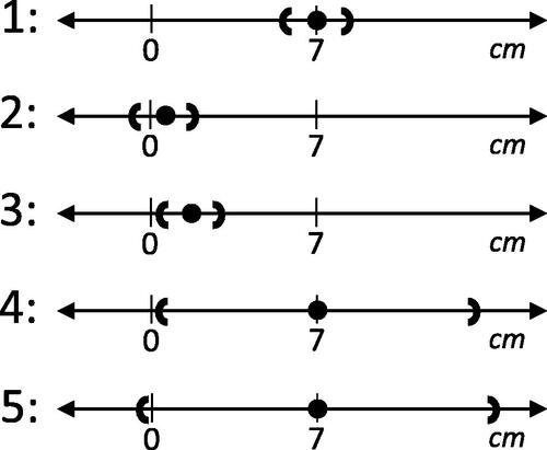
In Case 1, the estimate is precise and large enough to be interesting. Regarding statistical significance, consider testing the null hypothesis that the true parameter is zero versus the alternative hypothesis that the true parameter is not equal to zero, at a 5% level. We reject the null if the CI does not include zero. Thus, in Case 1 we reject the null, establishing statistically significant evidence that the parameter is not equal to zero.

In Case 2, we do not reject the null (the CI includes zero). Since the CI is narrow, this outcome is sometimes called a precise zero. Although the result is not statistically significant, it constitutes strong evidence that the parameter is less than five (the smallest interesting effect size). In terms of magnitude and precision, Cases 2 and 3 provide very similar information despite yielding opposite hypothesis test results. In Case 3, we reject the null even though the estimate is small in magnitude. Here statistical significance does not imply practical significance, like the one centimeter difference in corn height from Section 2.

The estimates in Cases 4 and 5 are significant in practical terms but come with substantial sampling uncertainty. Again, despite providing very similar information, they yield opposite hypothesis test results: we reject the null in Case 4 but not in Case 5. Comparing Case 4 with Case 1, both depict the same point estimate and both are statistically significant, but they differ enormously in precision. Case 1 provides evidence that the parameter is near seven, but in Case 4 the CI extends from just above zero to just under 14.

Regarding Case 5, failure to reject the null is sometimes mistakenly viewed as an acceptance of the null. In other words, finding no statistically significant effect is viewed as evidence that the parameter is zero. In Case 2 that conclusion may be reasonable. But more often, failure to reject simply indicates the results are inconclusive, as in Case 5 where the CI extends from slightly negative to greater than 14. Suppose Case 5 represented an association between a food additive and cancer in laboratory animals. Although we would not reject the hypothesis that there is no relationship, it would be difficult to find a statistician willing to consume the substance.

3.2 Implications

These five cases illustrate how hypothesis test outcomes, in isolation, do not provide all the information required to evaluate a result. Statistical significance is not a proxy for magnitude or precision. CIs provide a useful way to gauge precision while avoiding the potentially confusing terminology of hypothesis testing.

What constitutes sufficient precision? This assessment is tied to the evaluation of practical significance and must also be based on domain-specific knowledge. One rule-of-thumb is to require the margin-of-error to be less than the smallest magnitude of practical significance. In the corn fertilizer example, an estimate would need a margin-of-error of less than five to be considered precise. The assessment should also account for the fact that it is more difficult to obtain precise estimates in some contexts. So the judgment should consider the level of precision attained in related research. An imprecise estimate may still be informative: suppose the fertilizer were estimated to increase average plant height by 12 cm with a margin-of-error of 6 cm. Then, despite having a wide CI, its lower bound still represents a magnitude of practical importance.

Studies that involve data collection must start by specifying a required level of precision. This specification should then be used to calculate minimum sample sizes. The target level of precision is often stated as a margin-of-error or a level of statistical power. Statistical power is the probability of correctly rejecting a null hypothesis when a specific alternative hypothesis is true. Statistical power is a function of both sample size and the hypothesized parameter values (i.e., effect size). Thus, power analysis requires considering both precision and magnitude. In medical research, grant agencies commonly require sample sizes that yield statistical power of at least 80%.

In summary, statistical significance does not guarantee that an estimate is precise. In contrast, CIs provide an intuitive way to quantify precision. One possible benchmark is to consider an estimate’s margin-of-error relative to the smallest parameter value with practical significance. Finally, projects that involve collecting data should start by defining the required level of precision; minimum sample sizes can then be set accordingly.

4 Model Uncertainty

Of the three questions posed in Section 1, whether a model is correctly specified is the most difficult. It is also crucial because point estimates and CIs depend on the validity of the model. Sampling uncertainty is only one component of the overall uncertainty associated with an estimate. I define “model uncertainty” broadly to encompass all other sources of ambiguity. The research process requires making many decisions and the correct choice is often unknown.

Researchers tackle questions like: What explanatory variables should enter the statistical model? What is an appropriate functional form? What are the properties of the error term? Are standard approximations (e.g., asymptotic results for sampling distributions) adequate in a particular research context? Do the observable variables accurately represent the underlying theoretical constructs, for example, are wages an acceptable proxy for worker productivity? What is the proper way to handle data integrity issues such as missing or implausible values? A researcher’s answers to these questions are modeling assumptions.

To assess model uncertainty, first identify the modeling assumptions. Second, judge the validity of the assumptions. Third, check how key findings change in response to alternative modeling choices. Let’s consider each task in turn.

Modeling assumptions (including all the choices from model specification to sample selection and the handling of data issues) should be sufficiently documented so independent parties can critique, and replicate, the work. The assumptions most often overlooked may be the formal conditions attached to statistical models. To the benefit of applied researchers, statisticians derive the required conditions for valid estimates and CIs in specific contexts. For example, a method of computing a CI may require that unobserved factors are uncorrelated across observations. Researchers should consult statistical references to ensure they understand the assumptions associated with their models and methods.

Armed with a list of modeling assumptions, the next question is whether they are valid. Since it is rare for every condition to be completely satisfied, asking if a model is correctly specified actually means asking whether the model is adequate given the research goal. Are any assumptions sufficiently violated to cast doubt on the results? For instance, even after random assignment, the treatment and control groups in an experiment typically differ to some degree in their observable attributes. Are there also differences in unobserved factors? If so, are they substantial enough to confound the results?

To assess the plausibility of modeling assumptions, researchers rely on both theory and evidence. A scatterplot may show that it is reasonable to assume a linear relationship between height and age for elementary school children. Since empirical evidence is not always available, researchers also appeal to theory. Suppose I am estimating the impact of a job training program on wages for high school graduates. Can I simply compare the wages of the graduates who complete the training to the wages of typical high school graduates? In theory, factors such as diligence and motivation influence both earnings and the completion of a job training program. If so, then individuals who finish the training would have earned higher wages even without the program, so the simple difference in average wages would exaggerate the impact of training.

The third step in assessing model uncertainty is to check how estimates change across a range of plausible modeling and data choices. This sensitivity analysis is especially crucial when neither theory nor evidence points to one modeling approach over another. Robustness checks may be conducted using a formal framework such as Bayesian model averaging (Hoeting et al. 1999) or in an ad hoc manner such as using different functional forms and sets of explanatory variables. If a key finding disappears due to a seemingly arbitrary adjustment to the model, then the evidence for the finding is weak.

In summary, the first step when assessing model uncertainty is to identify the modeling assumptions. Assumptions include both formal conditions required by statistical models as well as more judgment-based choices such as sample selection and how to handle data integrity issues. The second step is to assess the validity of the assumptions. Researchers use theory and prior empirical results to support their modeling choices, so subject matter expertise it is especially crucial here. The third step is to assess the degree to which key findings change across model variations.

5 Conclusion

As a method of inquiry, the process of systematic observation, statistical analysis, peer review, and replication is undeniably effective. Still, the results from individual studies are usually not definitive. Researchers must clearly communicate the sampling and modeling uncertainties associated with their findings. The evaluation of an empirical result should take into account existing evidence on the topic. Is the research community approaching consensus or is there still considerable debate on the issue? When presenting research to audiences who lack subject matter knowledge, it is crucial to provide the context for evaluating the importance and the strength of the evidence.

Acknowledgments

The opinions expressed in this article are those of the author alone, and do not necessarily reflect the views of the Office of the Comptroller of the Currency or the U.S. Department of the Treasury. The author thanks Mike Anderson, Anna Hill, Ron Wasserstein and the referees for helpful comments.

Appendix: A Common Misinterpretation of Confidence Intervals

Section 3 defines CIs in frequentist statistics. It makes clear that the probability statement applies before the sample has been drawn. If a researcher has already drawn a random sample, obtained a point estimate and computed its 95% CI, then it is incorrect to say there is a 95% chance the true parameter lies within that specific interval. This is mistaken because the population parameter is not typically considered random, so it has no probability distribution. The realized bounds of a CI are also not random. Before the sample was drawn, the bounds were random variables (functions of a random sample). But after drawing the sample the realized bounds are not random (just as the roll of a die is random, but the result from a particular role is a constant). In short, after drawing the sample, nothing is random so probability statements do not make sense. The population parameter is either inside or outside the realized interval (and since the true parameter value is unknown, we cannot say which is the case).

One way to describe realized bounds is to refer to two implied hypothesis tests. Suppose an estimate has a 95% CI of [a, b]. Then, using a two-sided hypothesis test at the 5% level, we would not reject the null hypothesis that the population parameter is equal to a. In a separate test, we would not reject the hypothesis that it is equal to b. In this sense, the data is consistent with true parameter values ranging from a to b.

References

- Hoeting, J. A., Madigan, D., Raftery, A. E., and Volinsky, C. T. (1999), “Bayesian Model Averaging: A Tutorial,” Statistical Science, 14, 382–417.
- McCloskey, D. (1983), “The Rhetoric of Economics,” Journal of Economic Literature, 21, 481–517.
- McCloskey, D., and Ziliak, S. (1996), “The Standard Error of Regressions,” Journal of Economic Literature, 34, 97–114.
- Wasserstein, R. L., and Lazar, N. A. (2016), “The ASA’s Statement on p-Values: Context, Process, and Purpose,” The American Statistician, 70, 129–133. DOI: 10.1080/00031305.2016.1154108.
- Ziliak, S. T., and McCloskey, D. N. (2004), “Size Matters: The Standard Error of Regressions in the American Economic Review,” The Journal of Socio-Economics, 33, 527–546. DOI: 10.1016/j.socec.2004.09.024.