An Introduction to Second-Generation p-Values

ABSTRACT

Second generation p-values preserve the simplicity that has made p-values popular while resolving critical flaws that promote misinterpretation of data, distraction by trivial effects, and unreproducible assessments of data. The second-generation p-value (SGPV) is an extension that formally accounts for scientific relevance by using a composite null hypothesis that captures null and scientifically trivial effects. Because the majority of spurious findings are small effects that are technically nonnull but practically indistinguishable from the null, the second-generation approach greatly reduces the likelihood of a false discovery. SGPVs promote transparency, rigor and reproducibility of scientific results by a priori identifying which candidate hypotheses are practically meaningful and by providing a more reliable statistical summary of when the data are compatible with the candidate hypotheses or null hypotheses, or when the data are inconclusive. We illustrate the importance of these advances using a dataset of 247,000 single-nucleotide polymorphisms, i.e., genetic markers that are potentially associated with prostate cancer.

KEYWORDS:

• Likelihood ratios
• Null hypothesis
• p-Value
• Statistical evidence

ABSTRACT

Second generation p-values preserve the simplicity that has made p-values popular while resolving critical flaws that promote misinterpretation of data, distraction by trivial effects, and unreproducible assessments of data. The second-generation p-value (SGPV) is an extension that formally accounts for scientific relevance by using a composite null hypothesis that captures null and scientifically trivial effects. Because the majority of spurious findings are small effects that are technically nonnull but practically indistinguishable from the null, the second-generation approach greatly reduces the likelihood of a false discovery. SGPVs promote transparency, rigor and reproducibility of scientific results by a priori identifying which candidate hypotheses are practically meaningful and by providing a more reliable statistical summary of when the data are compatible with the candidate hypotheses or null hypotheses, or when the data are inconclusive. We illustrate the importance of these advances using a dataset of 247,000 single-nucleotide polymorphisms, i.e., genetic markers that are potentially associated with prostate cancer.

1 Introduction

By now everyone has seen the little red badges that appear on mobile phone apps and computer icons when the software wants attention. Besides stimulating serotonin production, those little red badges serve an important role: they notify the user when their attention is required. Perhaps not surprisingly, p-values have become the little red badges of applied statistics; they are assumed to indicate when the observed data are sufficiently informative to warrant the reader’s attention. The results, after all, have been deemed “significant.”

Having a gross indicator for when a set of data are sufficient to separate signal from noise is not a bad idea. The problem is that p-values perform poorly in this role. They confound effect size and precision, blurring the natural emphasis on meaningful effect sizes. They depend on the planned experimental design, even if the plan was not followed. Their proper interpretation is awkward. They are not consistent with the more intuitive measures of statistical evidence that arise in likelihood (Barnard 1949; Royall 1997; Blume 2002), Bayesian (Edwards, Lindman, and Savage 1963; Kass and Raftery 1995), and information theory (Good and Osteyee 1974) paradigms. In practice, these flaws often overshadow the p-value’s positive attributes (Berger and Sellke 1987; Blume and Peipert 2003; Greenland et al. 2016; Goodman 1993; Cornfield 1966; Royall 1986; Dupont 1983).

For decades now, the statistical community has discouraged researchers from perseverating on the significance level of new findings (Wasserstein and Lazar 2016). Instead, the community seems to favor a more holistic approach that surveys the available evidence, modeling choices, potentially impactful effect sizes, and scientific context. While this emphasis is generally welcomed by practitioners of statistics, it is hard to condense it into a single metric that can be uniformly applied across different disciplines. Efforts to replace the p-value with something else—for example, a likelihood ratio (LR, Royall 1997; Blume 2002), Bayes factor (Bayarri et al. 2016), or posterior probability (Spiegelhalter, Abrams, and Myles 2004; Edwards, Lindman, and Savage 1963)—have not yet garnered a large enough following to alter the daily practice of statistics in applied disciplines (e.g., Cristea and Ioannidis 2018). p-Value “improvements” have been limited to revising the threshold for significance (Johnson 2013; Benjamin et al. 2018; Lakens et al. 2018) and tweaking the interpretation (Ioannidis 2018). Unfortunately, these efforts, resurrected every few decades since the 1960s (Berkson 1942; Cornfield 1966; Cohen 1994; Savage 1962; Morrison and Henkel 1970), have not led to changes in the daily practice of statistics.

The need for a reliable descriptive summary of the statistical evidence at hand remains unmet. Science looks to statistics for a global assessment—a single number summary—of whether the data favor the null hypothesis, the alternative hypothesis or whether the data are inconclusive. More nuanced assessments are, of course, encouraged. But this does not eliminate the need for a quick and coarse assessment of what the data say that is uniformly applicable across disciplines.

The second-generation p-value (SGPV) was developed with this need in mind (Blume et al. 2018). The idea was to improve on the p-value, rather than discard it. This meant keeping familiar characteristics, such as the bounds of zero and one, while also adding new capabilities, such as the ability to indicate when the data support the null hypothesis. By construction, the SGPV retains many of the desirable properties of the p-value, incorporates often-wished-for properties, retains excellent control over error rates, operates with low false discovery rates (FDRs), and is readily interpretable by non-statisticians. In a broad sense, the SGPV simply indicates when experimental data support only the null premise or scientifically relevant alternative hypotheses.

The purpose of this note is to introduce the SGPV in a nontechnical manner and explain how it differs from the classical p-value. We will take the phrase “statistical inference” to mean measuring the strength of evidence in observed data about scientific hypotheses. Other inferential domains, such as belief theory (“What do I believe now that I have seen these data?”) and decision theory (“What should I do now that I have seen these data?”) will not be directly addressed. The focus here is on the most obvious and most frequently asked question in science: “Which scientific hypotheses are supported by the data?” Before introducing and discussing the SGPV, it is important to consider the conceptual framework that allows us to properly evaluate the statistical properties of the SGPV and to examine the manner in which we typically construct the null hypothesis.

2 Evidential Metrics

The majority of scientific activity consists of reporting and interpreting data as scientific evidence. Although there is no generally accepted mathematical framework for conducting an evidential analysis, there are three key metrics that comprise an evidential framework (Blume 2011):

1. A numerical assessment of the strength of evidence in a given body of observations

2. The probability that the numerical assessment will be misleading in a given setting

3. The probability that an observed assessment—one computed from observed data—is mistaken

The first metric is the scale of evidence, the second is the error rate, and the third is the FDR. These three metrics, obviously distinct, must be clearly defined for the evidential framework to be coherent. Failure to accomplish this creates a fatal flaw. Let’s take a moment to consider each metric’s role in the scientific process.

The first evidential metric is the numerical assessment of the strength of evidence in a given body of data. It is the researcher’s essential tool for understanding what the data say. This tool is typically justified by axiomatic or intuitive means. Typically, they are single number summaries, but there is no restriction that this always be the case. Suppose we use $\mathcal{M}$ to measure the strength of evidence. It might be a metric that indicates absolute support for, or against, a single hypothesis such as a p-value or posterior probability. Or, it might be a measure that indicates relative support for one hypothesis over another such as a LR, Bayes factor, or divergence measure. A simple point estimate, such as a mean difference, relative risk, or odds ratio, is not itself an evidential metric because the connection between the point estimate and candidate hypothesis is not formalized. After collecting data, we compute and report $\mathcal{M}$.

Sometimes the data, by way of its interpretation through $\mathcal{M}$, indicate support for a false hypothesis or indicate that the data are inconclusive. Neither outcome is desirable, so studies are designed to minimize the rate at which they generate misleading or inconclusive evidence. Accordingly, the second evidential metric is the propensity to observe undesirable outcomes such as misleading or inconclusive evidence. In statistical lingo, these are often called “error” rates.

Suppose we have two competing hypotheses H_A and H_B. The classical frequency properties of a study design would be $P(\mathcal{M}$ supports $H_A|H_B$), $P(\mathcal{M}$ supports $H_B|H_A$), $P(\mathcal{M}$ yields inconclusive evidence $|H_B$), and $P(\mathcal{M}$ yields inconclusive evidence $|H_A$). A good study design minimizes these probabilities to the best extent possible. There are, of course, many different statistical and experimental strategies for doing this. The key point is that these probabilistic measures are properties of the experiment, not properties of the data that result from the experiment. For this we need another tool.

Once the data are collected, we compute and report $\mathcal{M}$. We will know if the evidence is strong or if it is inconclusive from the observed value of $\mathcal{M}$. For example, the observed LR might be 100, which would represent very strong evidence favoring one hypothesis over another. However, we will not know if $\mathcal{M}$ is misleading or not. The third evidential metric is the propensity for observed evidence to be misleading; it is an FDR. The FDR is an essential complement to the first evidential metric. We report the observed metric to describe the strength of evidence in the observed data, and we report the FDR to describe the chance that this result is mistaken. Note that, unlike the second evidential metric, the FDR is a property of the observed data.

Continuing with the example, the FDRs would be $P(H_B|\mathcal{M}$ supported H_A) and $P(H_A|\mathcal{M}$ supported H_B). Bayes’ theorem must be used to compute these probabilities, so assumptions are made about the likelihood of the candidate hypotheses being true. The key insight is that once data are observed, it is the FDRs that are the relevant assessments of uncertainty. The error rates of the study design, critical at the design phase, are no longer relevant for the interpretation of observed data as statistical evidence. Rather it is the FDRs that convey the magnitude of uncertainty for the observed data.

The FDR was not formalized in the statistical literature until fairly recently (Benjamini and Hochberg 1995; Storey 2002, 2003). This is largely why statisticians and applied researchers have been slow to adopt this quantity in its natural role; preferring instead to rely on familiar but flawed interpretations of the Type I and Type II error rates. While it is true that the FDRs depend on the error rates (Wacholder et al. 2004), the FDRs are clearly distinct quantities and they should be treated as such.

A very successful real-world example of this structure comes from diagnostic medicine. Consider using CD4 count to determine if a patient, already infected with HIV, has developed AIDS. The CD4 count is an estimate of the number of active Helper T cells, per cubic millimeter, that can fight an infection. Normal CD4 counts range from 500 to 1500. When the CD4 count falls below 200, it is an indicator that the patient may have developed AIDS. Suppose we take $\mathcal{M}$ to be a LR and patient X is found to have a CD4 count of 150. Is this CD4 count, which supports a diagnosis of AIDS, strong evidence that patient X has AIDS? To answer this question, we compute the metric, say ${\mathcal{M}}_{\text{obs}}=50$, and interpret. The answer is yes; patient X’s LR is large and favors the hypothesis that the patient has AIDS. For simplicity here, let’s suppose the LR is a smoothly decreasing function of the CD4 count so we can forgo the actual computation of $\mathcal{M}$ and just use CD4 count as a surrogate for $\mathcal{M}$.

The second evidential metric—the properties of the diagnostic test—consist of sensitivity P(CD4 $\le 200|$AIDS) $=0.9$ and specificity P(CD4 $>200|$No AIDS) $=0.96$ (the numerical values were chosen for illustration purposes and do not reflect actual performance). Good diagnostic tests have high sensitivity and high specificity. The classical Type I and Type II error rates are the complements of these numbers, so $\alpha =0.04$ and $\beta =0.1$. When a physician receives patient X’s test results, she reports the observed CD4 count (e.g., CD4 $=150$) and the probability that the patient has AIDS given their CD4 count is below 200. This latter quantity is called the positive predictive value of the test result, P(AIDS—CD4 $\le 200)=$ PPV. We use Bayes’ theorem to compute the PPV from the test’s sensitivity and specificity if we know the disease prevalence, say 20% for illustration. Then, we see that PPV $=0.9\times 0.2/(0.9\times 0.2+.004\times 0.8)=0.85$. The FDR is simply 1 – PPV or P(No AIDS—CD4 $\le 200)=0.15$; it is the probability that patient X does not have AIDS when their CD4 count is less than 200.

In this context, it makes little sense for the physician to report to patient X the complement of the observed specificity, say P(CD4 $\le 150|$No AIDS) $=0.02$. This is because the patient already knows their CD4 count. Moreover, the patient really wants to know how likely it is that they have AIDS or, if that is not possible, whether their chances of having AIDS has increased now that their CD4 count is known. The rub is that the complement of specificity is the p-value. And it is not at all clear what the p-value adds beyond the observed CD4 count (150) and FDR (15%). Perhaps the physician should report the p-value and the PPV? Or perhaps the CD4 count and the p-value? Neither is quite right. This example illustrates why statistical inference based on p-values can be so confusing. Imagine what would happen if the p-value had to be adjusted for all the HIV tests run at the doctor’s office that day. Once data have been observed, it is the FDR that provides the correct assessment of uncertainty in the evidence; not the p-value.

Failure to distinguish between the evidential metrics leads to circular reasoning and irresolvable confusion about the interpretation of data as statistical evidence (Blume and Peipert 2003; Blume 2011). This is the fundamental dilemma that belies the p-value. Is the tail area probability a measure of the strength of evidence against the null hypothesis, or is it the study’s effective error rate? Nearly a century after Fisher and Neyman first argued this very point, it remains unclear with divergent opinion on the matter. Fisher would argue for the former and Neyman for the latter, but neither view has carried the day (Royall 1997; Berger 2003). The problem is that there is only one number, the tail area probability, and this one number is used to represent two different concepts. The conflation of these concepts, as they pertain to the tail area probability, is the genesis of the multiple comparisons/multiple looks paradoxes in statistics (Blume and Peipert 2003; Royall 1997). Fisher understood this, writing “In fact, as a matter of principle, the infrequency with which, in particular circumstances, decisive evidence is obtained, should not be confused with the force, or cogency, of such evidence” (Fisher 1959, p. 93). But this warning seems to have been long forgotten.

The SGPV framework respects the conceptual distinctions critical to a coherent evidential framework (Blume et al. 2018). As we will see, the SGPV is a proportion, not a tail area probability. This helps differentiate the summary of the strength of evidence in a given body of observations—the SGPV—from the design’s error rates and the data’s FDRs. The mere separation is a substantial inferential advance.

3 Specifying the Null Hypothesis

The SGPV is dependent on an expanded null hypothesis. The idea is to use a composite null hypothesis that reflects the limits on physical or experimental precision in outcome measurements, measurement error, clinical significance, and/or scientific relevance. Interval null hypotheses are constructed by incorporating this information into statistical hypotheses that are stated a priori. For example, when follow-up intervals are limited to weeks, it makes little sense to ponder survival differences of 7 days or less; that level of resolution for the outcome is too high given that the data were collected on a weekly basis. So, the natural interval null hypothesis consists of survival differences of 7 days or less. The interval null should contain, in addition to the precise point null hypothesis, all other point hypotheses that are practically null and would maintain the scientific null premise. While the hypotheses in the interval null may be mathematically distinct, they are all considered scientifically equivalent to the null premise. Examples include:

• $H_0:0.95\le \text{OR} \le 1.05$ instead of $H_0: \text{OR} =1$,

• $H_0:-0.1\le P(\text{Survival}|\text{Group}1)-\mathrm{P}(\text{Survival}|\text{Group}2)\le 0.1$ instead of $H_0:P(\text{Survival}|\text{Group}1)-\mathrm{P}(\text{Survival}|\text{Group}2)$, and

• $H_0:-0.5\sigma \le {\mu }_1-{\mu }_2\le 0.5\sigma$ instead of $H_0:{\mu }_1={\mu }_2$.

By using an interval null hypothesis, we focus the evidential assessment on scientifically relevant effects. As a consequence, the Type I error rate, held constant in classical frequentist inference, naturally converges to zero as the sample size grows (see Section 5). The disadvantage is mainly procedural; it takes real forethought to specify the width of the interval in advance (Remark A). However, the extra effort does have a payoff. Findings that rule out this interval are both statistically significant and scientifically impactful. They are generally more reliable (the FDR is lower), and they are more likely to reproduce in subsequent studies. The reason for this is that the vast majority of Type I errors occur close to the point null hypothesis (2–4 standard errors away). Ergo, establishing a “buffer zone” translates into a substantial reduction in the rate of false discoveries.

In effect, the switch to an interval null hypothesis eliminates the common problem that classical statistical significance does not imply scientific relevance. This has been known in the statistical literature for some time. For example, Lehmann (1986, secs. 4.5 and 5.2; Good 2007) point out that the infinite precision of a point null hypothesis is rarely required (or justified) in practice. The scientific translation of this is that rejecting the null hypothesis that two effects are identical is largely not helpful, because they could still be nearly identical for all practical purposes. It is more helpful to establish that the effects differ by a meaningful amount. Unfortunately, current practice is to make this assessment after the data are analyzed, when it is easier to be influenced by the observed results. The SGPV approach requires that this assessment be determined before the data are collected and therefore justified by scientific reasoning independent of the observed data, adding an important layer of rigor to the analysis.

4 The Second-Generation p-Value

The SGPV seeks to measure the fraction of data-supported hypotheses that are also scientifically null hypotheses. We will denote the SGPV by $p_{\delta }$ to signal its dependence on the interval null and distinguish it from the classical p-value (Blume et al. 2018). To identify the collection of “data-supported hypotheses,” we use an interval estimate such as a confidence interval (CI), a likelihood support interval (SI), or a credible interval. Any type of interval may be used, but the choice impacts the frequency characteristics of the SGPV (see Remark B). In this article, we will use 1/8 likelihood SIs, which have numerous favorable inferential properties (Blume 2002; Royall 1997). Briefly, a 1/8 SI often corresponds to the traditional 95.9% Wald CI. As such, 1/8 SIs can be thought of as slightly conservative 95% CIs that do not need to be adjusted for sample space considerations (Blume 2002). Remark C provides a formal definition of SIs and an example.

Suppose that we are interested in the value of some parameter θ. Let $I=[{\theta }_l,{\theta }_{\mathrm{u}}]$ be the interval estimate of θ whose length is given by $\left|I\right|={\theta }_{\mathrm{u}}-{\theta }_l$. Let the interval null hypotheses be denoted by H₀ and its length by $\left|H_0\right|$. The SGPV is(1) $$\begin{array}{c}{p}_{\delta }=\frac{|I\cap H_0|}{\left|I\right|}\times \max \left\{\frac{\left|I\right|}{2\left|H_0\right|},1\right\}\\ =\{\begin{array}{cc}\frac{|I\cap H_0|}{\left|I\right|}& \text{when} \left|I\right|\le 2\left|H_0\right|\\ \frac{1}{2}\frac{|I\cap H_0|}{\left|H_0\right|}& \text{when} \left|I\right|>2\left|H_0\right|\end{array}\end{array}$$(1) where $I\cap H_0$ is the intersection or overlap of the two intervals. When the data are sufficiently precise, the SGPV is the fraction of I that is in H₀, i.e., $p_{\delta }=|I\cap H_0|/\left|I\right|$. Here, “sufficiently precise” means that the interval estimate is not more than twice the width of the interval null, that is, when $\left|I\right|\le 2\left|H_0\right|$.

When the interval estimate is very wide with $\left|I\right|>2\left|H_0\right|,I$ often extends on either side of H₀. In these cases, the quantity $|I\cap H_0|/\left|I\right|=\left|H_0\right|/\left|I\right|$ tends to be small and does not properly reflect the inconclusive nature of the data. The correction term $\max \left\{\frac{\left|I\right|}{2\left|H_0\right|},1\right\}$ replaces the denominator $\left|I\right|$ with $2\left|H_0\right|$ so that $p_{\delta }=0.5\times |I\cap H_0|/\left|H_0\right|$, which is bounded by 1/2. Note that $p_{\delta }$ can still be small despite being shrunk to 1/2 if the overlap $|I\cap H_0|$ is small. The correction factor maps inconclusive data toward a SGPV of 1/2, reserving magnitudes near 1 for data that support the null premise. This behavior is different than in traditional p-values, where large p-values result when data are inconclusive (i.e., when the CI is wide) and when the data support the null hypothesis (i.e., when the CI is tight around the null hypothesis).

Figure 1 illustrates how SGPVs work (reproduced from Blume et al. 2018). The overlap between the interval estimate (here a CI, but easily imagined as a SI) and the interval null is the essence of the SGPV. When the interval estimate is contained within the null interval, the data support only null hypotheses and $p_{\delta }=1$. When the interval estimate and null set do not overlap, the data are said to be incompatible with the null and $p_{\delta }=0$. When the null set and CI partially intersect, $0<p_{\delta }<1$ and the data are inconclusive. In this last case, $p_{\delta }$ communicates the degree of inconclusiveness. For example, when $p_{\delta }\approx 1/2$, the data are said to be strictly inconclusive. But different levels of inconclusiveness are possible. For example, when $p_{\delta }\approx 0.2$, the data might be interpreted as trending in support of certain alternative hypotheses. When $p_{\delta }\approx 0.1$, the data might be interpreted as suggestive of a scientifically meaningful effect but not definitively. When $p_{\delta }\approx 0.01$ or $p_{\delta }\approx 0.99$, the data are close to fully supporting some alternative hypotheses or the null premise, respectively. While the descriptors of SGPV magnitude are helpful as communicators, they are not as essential as they are to traditional p-values because the natural ending states are well defined as $p_{\delta }=0$ or 1 (Remark D).

Fig. 1 Illustration of a point null hypothesis, H₀; the estimated effect that is the best supported hypothesis, $\widehat{H}=\widehat{\theta }$; the confidence interval (CI) for the estimated effect [${\text{CI}}^{-},{\text{CI}}^{+}$]; and the interval null hypothesis $[H_0^{-},H_0^{+}]$.

To illustrate, consider a study of 100 smokers and 100 nonsmokers, where 65 smokers and 50 nonsmokers developed lung cancer. These data yield an odds ratio of 1.86 for the association of smoking and lung cancer. It is generally thought that odds ratios between 0.9 and 1.1 are too small to lead to meaningful associations. These data result in a 1/8 SI (95.9% CI) for the odds ratio of 1.03–3.36. The SGPV would then be $p_{\delta }=0.175=\left(\frac{1}{2}\right)\frac{(1.1-1.03)}{(1.1-0.9)}$ because the width of the CI is more than twice that of the null interval. The natural overlap measure is adjusted from $\frac{(1.1-1.03)}{(3.36-1.03)}=0.03$ to 0.175 to reflect that the data are relatively imprecise when the goal is to learn about an interval null as tight as 0.9 to 1.1. With a $p_{\delta }=0.175$, we would report that the study yielded inconclusive results. However, if 70 rather than 65 smokers developed lung cancer the odds ratio would be 2.33 with a 1/8 SI of 1.27–4.27. Now the intervals do not overlap so $|I\cap H_0|=0$. Hence, $p_{\delta }=\left(\frac{1}{2}\right)\frac{(0)}{(1.1-0.9)}=0$ and we would report that the data support a scientifically meaningful association between smoking and lung cancer.

The SGPV can be viewed as a formalization of today’s standard practice of using CIs to assess the potential scientific impact of new findings. In our view, it is much better to make these judgment calls about scientific impact before looking at the data. SGPVs are intended as summary statistics that indicate when a study has yielded a CI that supports only the null premise or meaningful alternative hypotheses. By focusing only on results that are scientifically meaningful, the SGPV changes the relative importance of statistically significant findings. This means that the findings associated with the smallest p-value(s) will not necessarily have a corresponding SGPV of 0, nor will they necessarily correspond to the top ranked SGPVs. This is illustrated nicely in our high-dimensional genetics example (Section 6).

Table 1 provides a side-by-side comparison of the properties of classical p-values and SGPVs. The take home message is that the SGPV is essentially an upgraded classical p-value.

Table 1 Comparison between the classical and second-generation p-value.

Property	Classical p-value	Second-generation p-value
Null hypothesis	Point	Interval
Scale	Number between 0 and 1, excluding zero	Number between 0 and 1, inclusive
Able to indicate support for alternative hypotheses	When small or near 0	When 0
Able to indicate data are inconclusive	When larger than the stated cutoff for significance	When between 0 and 1; near 1/2 is strictly inconclusive
Able to indicate support for null hypotheses	No	When 1
Accounts for practical importance	No	Yes, via specification of the null
Comparable across datasets	Yes, when the sample size is equal	Yes, when the width of the interval null is equal
Interpretation	Awkward, conditions on null hypothesis	Straightforward, conditions on observed data
Assumptions needed for computation	Probability model, sharp null hypothesis, sample space	Probability model, interval null hypothesis
Requires threshold for interpretation	Generally, yes	No, intended as a descriptive statistic
Adjustments required for multiple comparisons/looks?	Yes, if considered a Type I error rate; no, if considered a measure of statistical evidence	No

Lastly, two endpoints with a SGPV of zero $(p_{\delta }=0)$ are compared on the basis of their delta-gap (Blume et al. 2018). The delta-gap is the distance between the null interval and the likelihood SI in units of δ, where δ is the half-width of the interval null hypothesis. For example, when the SI is shifted to the right of the null interval, the δ-gap is (CI${}^{-}$ – $H_0^{+})/\delta$. The scaling by δ makes it unit free and therefore easy to compare. Comparisons of δ-gap favor larger effect sizes. We use the delta-gap to rank SGPV findings in Section 6.

5 Frequency Properties

Blume et al. (2018) shows why the frequency properties of SGPVs can be controlled through sample size. For convenience, we mention a few key results here. Let ${\widehat{\theta }}_n$ be a consistent estimator of parameter θ and assume an acceptable approximation to its sampling distribution is $\sqrt{n}({\widehat{\theta }}_n-\theta )\tilde{A}N(0,V)$, where the variance V is either known or can be readily estimated. This setting applies to most maximum likelihood estimators and posterior modes in large samples. When a $(1-\alpha )$ 100% CI is used as the interval estimate, the SGPV Type I error rate analogue is(2) $$P_{{\theta }_0}(p_{\delta }=0)=P(p_{\delta }=0|\theta ={\theta }_0)=2\Phi \left[-\frac{\sqrt{n}\delta }{\sqrt{V}}-Z_{\alpha /2}\right].$$(2)

Note the dependence on the sample size n and on δ. The Type I error rate remains bounded above by $\alpha =2\Phi [-Z_{a/2}]$. This is subtly different from Neyman–Pearson hypothesis testing with a composite null, where the size of the test is defined as the maximum Type I error rate over the null space (α). The SGPV approach anchors the Type I error at the natural experimental point null and uses the interval around the point null as a buffer. As such, when $\delta >0,P_{{\theta }_0}(p_{\delta }=0)$ shrinks to 0 as the sample size grows (instead of remaining constant at α). When δ = 0, we recover the usual constant Type I error rate of α. The derivation of $P_{\theta }(p_{\delta }=0)$, along with the probability that the data are compatible with the null, $P_{\theta }(p_{\delta }=1)$, and the probability that the data are inconclusive $P_{\theta }(0<p_{\delta }<1)$, can be found in Supplement 1 of Blume et al. (2018). Remark E provides an expression for $P_{\theta }(p_{\delta }=0)$, the SGPV power function.

Once data are collected and the SGPV is computed, the relevant uncertainty measure is the probability that the observed results, say $p_{\delta }=0$ or 1, are mistaken. These are known as the FDR, $P(H_0|p_{\delta }=0)$, and the false confirmation rate (FCR), $P(H_1|p_{\delta }=1)$. The hypothesis notation, H_i for i = 0, 1, is left flexible on purpose. It can represent either a point hypothesis, $H_i:\theta ={\theta }_i$, or a composite hypothesis $H_i:\theta \in {\Theta }_i$, as needed. For example, $P(p_{\delta }=0|H_0)=P_{{\theta }_0}(p_{\delta }=0)$ when $H_0:\theta ={\theta }_0$. Otherwise, $P(p_{\delta }=0|H_0)$ is the average rate over $H_0:\theta \in {\Theta }_0$, defined as $P(p_{\delta }=0|H_0)={\int }_{{\Theta }_0}{P}_{\theta }(p_{\delta }=0)g(\theta )\mathrm{d}\theta$, for some probability distribution $g(\theta )$ over ${\Theta }_0$. Bayes’ rule yields expressions for the FDR and FCR(3) $$\begin{array}{c}P\left(H_0\right|p_{\delta }=0)={\left[1+\frac{P(p_{\delta }=0|H_1)}{P(p_{\delta }=0|H_0)}\mathrm{r}\right]}^{-1}\\ P\left(H_1\right|p_{\delta }=1)={\left[1+\frac{P(p_{\delta }=1|H_0)}{P(p_{\delta }=1|H_1)}\frac{1}{r}\right]}^{-1}\end{array}$$(3) where $r=p(H_1)/P(H_0)$ is the prior probability ratio (Blume et al. 2018). These rates depend on the (possibly averaged) design probabilities $P(p_{\delta }=0|H_1),P(p_{\delta }=0|H_0),P(p_{\delta }=1|H_0),P(p_{\delta }=1|H_1)$, through the LR given the observed SGPV. Good designs—those with low probabilities of observing misleading evidence—will have low FDRs.

For fixed prior probability ratio r, the LRs $P(p_{\delta }=0|H_1)/P(p_{\delta }=0|H_0)$ and $P(p_{\delta }=1|H_0)/P(p_{\delta }=1|H_1)$ will drive the FDR and FCR to zero as the sample size grows. This is an improvement over the FDR from a classical hypothesis test, which remains constant in the limit: $\alpha /(\alpha +r)$. The convergence to zero of the SGPV’s FDR and FCR happens because the design probabilities, for example, $P(p_{\delta }=0|H_0)$, converge to zero. Thus, while it may not be possible to identify r, the prior’s influence can be mitigated through sample size and good study design. Lastly, it is worth repeating that the Type I error rate, $P(p_{\delta }=0|H_0)$, and the FDR, $P(H_0|p_{\delta }=0)$, are not exchangeable. Their magnitudes can vary substantially. See Blume et al. (2018) and its Supplement 1 for further details.

6 Links to Prostate Cancer in 247,000 SNPs

The International Consortium for Prostate Cancer Genetics (Schaid and Chang 2005; ICPCG 2018) collected data on 3,894 individuals of European descent, each with 4.6 million single-nucleotide polymorphisms (SNPs) available for analysis. Genetic ancestry and independence were confirmed in 2511 cases with prostate cancer and 1383 controls without prostate cancer. SNPs measure the number of variant alleles (0, 1, or 2) at a given position on a chromosome. Alleles with prevalence less than 50% in the population of interest are variant. SNPs are routinely used as genetic markers in studies of disease.

Our analysis focused on 246,563 SNPs from chromosome 6. We chose chromosome 6 because it contains a cluster of genetic variants in or near an organic cation transporter gene (SLC22A3) that are thought to be associated with prostate cancer. We used logistic regressions to obtain 246,563 estimated odds ratios with 1/8 likelihood SIs (95.9% Wald CIs). Odds ratios of small to moderate size are of interest in the context of genetic investigations of common disease. Accordingly, we defined the interval null hypothesis as odds ratios between 0.9 and 1.1111 (= 1/0.9), which is symmetric on the log scale. Remark F records pertinent scientific details.

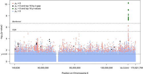
A Manhattan plot (Figure 2) displays the traditional p-values, at sequence chromosome position on chromosome 6 (Remark G), computed under the null hypothesis that the odds ratio is precisely 1. The Bonferroni cutoff $(p=2.03\times {10}^{-7})$, Benjamini–Hochberg FDR cutoff $(p=4.77\times {10}^{-6})$, and unadjusted cutoff (p = 0.05) are displayed as horizontal dashed lines. The points are colored according to SGPV status. There are 11,844 SNPs with p < 0.05, which accounts for 4.8% of all SNPs. Only 27 of these SNPs are statistically significant when controlling the FDR to 5%, and 16 of these meet the Bonferroni criteria. Importantly, all 27 of these SNPs are concentrated in or near the organic cation transporter gene (SLC22A3). These 27 SNPs also have a SGPV of zero $(p_{\delta }=0)$.

Fig. 2 Manhattan plot of SNP associations, colored according to second-generation p-value status. The x-axis shows SNP position on chromosome 6 and the position of the organic cation transporter gene (SLC22A3). The top 16 associations by p-value rank are in green and the top 16 associations by second-generation p-value rank are in black. Bonferroni, FDR, and unadjusted significance levels are show by dashed lines.

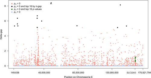
There are 1443 SNPs (0.6% of all SNPs) with $p_{\delta }=0$. For comparison with Bonferroni, we identified the top 16 SNPs according to their SGPV delta-gap rankings. The δ-gap measures the distance between the interval estimate and the null interval in units of δ (recall δ is the half width of the interval null). When $p_{\delta }>0$ the δ-gap is defined to be zero because there is no gap between the intervals. Figure 3 shows a modified Manhattan-style plot that displays the delta-gap by its position on chromosome 6. While the 16 Bonferroni SNPs can be seen concentrated around SLC22A3 (in green), the top 16 SNPs by δ-gap (black) are instead spread across the chromosome and potentially identify much stronger associations. In fact, the 16 Bonferroni SNPs are ranked between 423rd and 845th by the δ-gap metric, which illustrates that classical methods can disregard a large number of potentially impactful associations.

Fig. 3 Modified Manhattan-style plot of SNP associations as measured by the delta-gap. Points are colored according to second-generation p-value status. The x-axis shows SNP position on chromosome 6 and the position of the organic cation transporter gene (SLC22A3). The top 16 associations by p-value rank are in green and the top 16 associations by second-generation p-value rank are in black.

We can see in Figure 3 that the SGPV approach emphasizes the magnitude of the observed association in addition to classical statistical significance. SNPs with a SGPV of 0 also have a classical p-value that is less than 0.041 (the compliment of the coverage probability for the 1/8 SI). However, the converse is not true. Statistically significant findings can have an interval estimate that intersects with the interval null, leading to a SGPV > 0. Moreover, the δ-gap ranking orders findings by the weakest nonnull effect size supported by the data. Hence, the SGPV approach can be thought of as selecting for the potentially strongest nonnull statistically significant effects supported by the data, even when estimated relatively imprecisely.

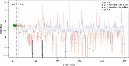
When comparing top ranked SNPs according to different criteria, it is helpful to examine the 1/8 SIs for the odds ratio relative to the null interval hypothesis. This is done in Figure 4, which displays the SNPs with the 500 smallest classical p-values, ranging from $5.01\times {10}^{-11}$ (rank 1) to 0.0016 (rank 500). The SNPs that met Bonferroni and FDR criteria reflect highly precise estimates of modestly sized odds ratios. Other SNPs that have similar effect sizes and levels of precision, for example, those immediately to the right of the FDR cutoff line, are ignored. Figure 4 also shows that there are many similarly precise SIs that are denoted as inconclusive by the SGPV (blue) because some null effects have not been ruled out.

Fig. 4 1/8 likelihood SIs for the estimated odds ratio for SNPs with the smallest 500 p-values. The x-axis is p-value rank. The interval null hypothesis (in gray) ranges from 0.9 to 1.1111 (= 1/0.9). Intervals are colored according to second-generation p-value status. The top 16 Bonferroni SNPs are in green and the top 16 SGPV SNPs are in black. Bonferroni (“Bonf”) and FDR significance levels are shown by dashed lines.

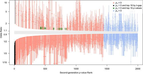
To further explore the differences in approaches, Figure 5 displays the top 2000 1/8 SIs as ranked by δ-gap when $p_{\delta }=0$, and by the SGPV when δ-gap $=0$ (hereafter referred to as SGPV rank). All 1,443 SNPs with a SGPV of 0 are sorted by their delta-gap and displayed in red. Intervals in blue have small but inconclusive SGPVs between 0 and 0.07 (often resulting from a very wide SI that just slightly overlaps the null interval). Notice the 16 Bonferroni SNPs (green) are in the middle of the plot, far from the top findings by SGPV. The estimated effects from the top ranked SGPV SNPs are clearly very large, but not precisely estimated. We also see that the top 16 ranked SGPVs finds associations in both directions, while the Bonferroni and FDR approaches only find associations in one direction. This figure makes it clear that the SGPV prioritizes the observed strength of association in findings that are statistically significant.

Fig. 5 Mirrored waterfall plot. 1/8 likelihood SIs for the estimated odds ratio for SNPs in the top 2,000 second-generation p-value ranking. The x-axis is SGPV rank. The interval null hypothesis (in gray) ranges from 0.9 to 1.1111 (= 1/0.9). Intervals are colored according to second-generation p-value status. The top 16 Bonferroni SNPs are in green and the top 16 SGPV SNPs are in black.

It is helpful to see if any correspondence exists between the classical p-value and the SGPV. Figure 6 shows their cross-tabulation. Of the 11,844 SNPs with p < 0.05, there are 1,443 that have a SGPV equal to 0. Another 2,622 are effectively inconclusive with SGPVs between 0.4 and 0.6, of which 783 have a SGPV greater than 0.5, indicating very weak support for the null rather than the alternative hypothesis. There are 3,377 SNPs with a SGPV of 1, indicating no association between SNP and cancer status, and they are uniformly dispersed across the chromosome with observed classical p-values of 0.76 or larger. This apparent correspondence should not be over interpreted; it is due to the relatively narrow interval null. As the width of the interval null lengthens, this relationship disappears. For example, when the interval null is expanded to 0.8 to 1.25 (= 1/0.8), there are 83,749 SNPs with $p_{\delta }=1$, and the classical p-values for these SNPs are evenly distributed from 0.007 to 1. This is not a typo; there are very precise intervals within the null region that exclude OR = 1 and these SNPs have very small classical p-values. But given their close proximity to OR = 1 they support the null premise better than alternative theories.

Fig. 6 Cross-tabulation of classical p-values and second-generation p-values in the prostate cancer data example.

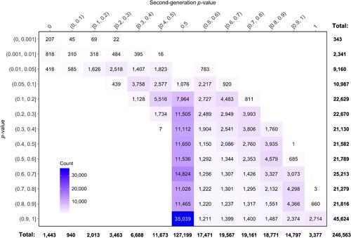
Another interesting aspect of Figure 6 is the large number of SGPVs at exactly 1/2. Many of these arise from logistic models with poor fit, often because there are one or more zero cells in the contingency table. Despite this, classical p-values near 1 are often still reported by software, whereas the SGPVs map these cases back to 1/2 (inconclusive). Of the 45,624 classical p-values greater than 0.9, almost half (47.6% or 21,697 cases) correspond to a SGPV of 1/2 because their point estimates were essentially undefined and estimated variances were extremely large. This reinforces the notion that large p-values do not imply the data support the null premise, even in large datasets.

For illustration, we computed several flavors of the FDR for 5 SNPs with a SGPV of 0. These are displayed in Table 2. Three versions of the $\text{FDR}=P(H_0|p_{\delta }=0)$ were computed. Here θ is the log odds ratio and $\widehat{\theta }$ is its MLE. FDR₁ uses the natural point null, $H_0:\theta =\hspace{0.17em}\text{log}\hspace{0.17em}(1)$, with the alternative set to the MLE, $H_1:\theta =\widehat{\theta }$. FDR₂ uses a point null hypothesis that is closer to the null boundary, $H_0:\theta =\hspace{0.17em}\text{log}\hspace{0.17em}(1.05)$, with a prespecified alternative $H_1:\theta =\hspace{0.17em}\text{log}\hspace{0.17em}(2)$. FDR₃ uses the interval null $H_0:\theta \sim \text{UNIF}[\text{log}\hspace{0.17em}(0.9),\hspace{0.17em}\text{log}\hspace{0.17em}(1/0.9)]$ and the interval alternative $H_1:\theta \sim \text{UNIF}[{\widehat{\theta }}_l,{\widehat{\theta }}_u]$ where ${\widehat{\theta }}_{\mathrm{l}}$ and ${\widehat{\theta }}_{\mathrm{u}}$ are the lower and upper bound of the 1/8 SI. FDR computations follow the formulas in Section 5 and Remark E.

Table 2 False discovery rates of 5 SGPV = 0 findings computed under various null and alternative hypothesis configurations.

			Odds	1/8 SI	1/8 SI
SNP ID	SGPV rank	p-Value rank	ratio	lower limit	upper limit	FDR1	FDR2	FDR3
kgp4568244_C	1	133	0.10	0.03	0.37	2.9%	17.1%	3.3%
kgp8051290_G	13	2002	15.58	1.95	124.68	4.3%	30.3%	4.9%
kgp4497498_A	28	255	4.37	1.80	10.64	2.5%	8.6%	3.1%
rs3123636_G	423	1	1.39	1.26	1.55	0.004%	0.1%	0.4%
kgp7460928_G	1443	3310	1.78	1.11	2.87	2.4%	2.0%	3.0%

NOTE: The prior probability ratio, r, is set to 1.

We see from these results that a decent first-order approximation is given by FDR₁, which is also straightforward to compute. All of the FDRs are low, as is expected from a SGPV = 0 finding (Remark H). Some are low because their 1/8 SI is shifted far from the null interval (2nd row), and some are low because their 1/8 SIs is very narrow (4th row, also the top finding by classical p-value) despite being only slightly shifted off the interval null. These calculations also illustrate why using the FDR alone is not best practice for ranking or screening findings. That strategy downplays the scientific importance of the estimated effect size and is sensitive to how the FDR is defined (as evidenced by FDR${}_2=30.3$% in row 2). Nevertheless, the FDR is essential when gauging the potential for a finding to be mistaken or misleading.

Lastly, an example global summary of the results is as follows:

Of the 246,563 SNPs examined in this analysis, 1,443 were found to have strong evidence of a meaningful association with cancer status (data supported ORs > 1.11 or < 0.9, SGPV $=0$). Another 3,377 SNPs were found to have practically no association with prostate cancer ( $0.9<$ ORs < 1.11, SGPV $=1$). The remaining 241,743 SNPs were inconclusive to varying degrees. There were 940 SNPs in which the data were suggestive of a meaningful association with cancer status but were unable to rule out trivial effects ( $0<$ SGPV $<0.1$). Similarly, there were 14,797 SNPs in which the data were suggestive of no association, but not strong enough to rule out meaningful effects ( $0.9<$ SGPV < 1). The remaining 226,006 SNPs were effectively inconclusive ( $0.1<$ SGPV < 0.9).

A detailed summary for individual SNP findings might be:

SNPs kgp4568244_C (1/8 SI for OR: 0.03–0.37, SGPV = 0) and kgp8051290_G (1/8 SI: 1.95–124.7, SGPV = 0) were the top ranked protective and harmful SNPs. SNPs rs9257135_G (1/8 SI: 0.92–1.09, SGPV = 1) and kgp10695421_A (1/8 SI: 0.91–1.1, SGPV = 1) were found to be unassociated with cancer status. SNP kgp17007117_A (1/8 SI: 1.08–3.6, SGPV = 0.07) was suggestive of a relationship, while findings for SNP kgp8948004_A (1/8 SI: 0.96–1.20, SGPV = 0.65) were inconclusive.

7 Comments and Remarks

The second-generation p-value (SGPV) provides the inferential properties that many scientists wish were attributes of the classic p-value. In addition, they are easy to interpret, they retain excellent frequency properties, they provide error rate control, and they have reduced false discovery rate (FDR). The prostate cancer example shows how SGPVs can be much more informative than classical p-values. Moreover, we saw that the Bonferroni procedure tends to find modest odds ratios for common variants, while SGPVs tend to identify the strongest associations that are both statistically significant and scientifically meaningful. This behavior was also observed in the high-dimensional example used in Blume et al. (2018). Changing culture so that we routinely specify internal null hypotheses before the study is conducted, as opposed to after, will be challenging. However, the rewards would be substantial; manifesting as increasing statistical reliability and increased scientific reproducibility of observed results. Prominent use of the second-generation p-value would encourage that type of culture shift, and both science and statistics would be better off for it.

Remark A.

In practice the best we can do is to encourage pre-specification of the null premise. Some scientific domains are better at this than others. For example, in clinical trials the study protocol is posted to clincialtrials.gov before the study enrolls patients. Nevertheless, the specification of the null premise is always an important scientific issue and recognizing that this should occur before analyzing the data is an important step forward for reproducibility and rigor.

Remark

B. Although the coverage probability of the interval estimate is not represented symbolically on $p_{\delta }$, it plays a major role in determining the frequency properties of $p_{\delta }$, that is, the error rates and FDRs. The connection is detailed in later sections. It is a key incentive to use intervals with good frequency properties (unbiasedness, shortest expected length, robust coverage, etc.) and to be transparent about why a certain type of interval was chosen.

Remark

C. For parameter θ, likelihood function $L(\theta )$ and MLE $\widehat{\theta }$, the 1/k likelihood SI is the set $\{\theta :L(\theta )/L(\widehat{\theta })\ge 1/k\}$. A SI is the collection of parameter values under the “hump” of the likelihood function when scaled by its maximum; these parameter values have nearly the same likelihood value as the maximum likelihood estimator (MLE) itself, and are “close” in that sense. When $X_1,\dots ,X_n\sim N(\theta ,{\sigma }^2)$ and ${\sigma }^2$ is known, the $1/k$ SI is ${\overline{X}}_n\pm \sigma \sqrt{2\hspace{0.17em}\text{log}\hspace{0.17em}(k)/n}$. When $k=8,\sqrt{2\hspace{0.17em}\text{log}\hspace{0.17em}(k)}=2.04$, and the 1/8 SI is equivalent to an unbiased 95.9% CI with shortest expected length. An advantage of SIs is that they often correspond to CIs that are desirable in some sense, for example, shortest expected length or unbiasedness. This discourages the use of nonstandard CIs that have the same coverage probability. See Royall (1997) and Blume (2002) for more on SIs.

Remark D.

SGPVs of 0 and 1 are intended to be clear endpoints. They do not imply overwhelming precision, but rather that the accumulated data support only meaningful alternative hypotheses or only practically null hypotheses. The label “suggestive” can be attached to SGPVs between 0 and 0.1 or 0.9 and 1, to describe data that may warrant further attention for ancillary reasons (e.g., limited resources). The key point, The key point is that SGPVs are summary measures to be used for facile communication of results; they should not replace examination of the interval estimate in the context of scientific discussions and policy decisions.

Remark

E. The power function for the SGPV is $P_{\theta }(p_{\delta }=0)=\Phi \left[\frac{\sqrt{n}({\theta }_0-\delta )}{\sqrt{V}}-\frac{\sqrt{n}\theta }{\sqrt{V}}-Z_{\alpha /2}\right]+\Phi \left[-\frac{\sqrt{n}({\theta }_0+\delta )}{\sqrt{V}}+\frac{\sqrt{n}\theta }{\sqrt{V}}-Z_{\alpha /2}\right]$ when the interval null is symmetric about θ₀. When $\theta ={\theta }_0$, this reduces to $P_{{\theta }_0}(p_{\delta }=0)$ in (2). This expression is needed for computation of FDRs.

Remark

F. The 246,563 SNPs investigated here were informative and not in strong local linkage disequilibrium. The Bonferroni correction is overly conservative when there is strong linkage disequilibrium (i.e., high correlation) among SNPs. To reduce this problem slightly, we identified bins of contiguous SNPs with an $R^2>0.98$ and eliminated all but one SNP from each bin. The number of variant alleles was treated as a continuous measure in the logistic models, which is standard practice.

Remark

G. SNP position was recorded as the number of nucleotides from the start of the p-arm of chromosome 6 based on reference assembly GRCh37/hg19.

Remark

H. FDR rates that result from a screening procedure based on p-values will be larger than those computed based on SGPV screening. For example, SNP rs3123636_G has the smallest p-value (4th row, Table 2), but its FDR under classical p-value screening inflates over 10-fold to $\sim 3.9\%$ for all three FDR flavors. Inflation occurs even when a multiple comparison correction, such as Bonferroni, is applied. Blume et al. (2018) provide details and an example.

Remark

I. A link to a repository of R functions for computing second generation p-values and associated quantities can be found on www.statisticalevidence.com, GitHub https://github.com/weltybiostat/sgpv, or by contacting the corresponding author.

References

- Barnard, G. (1949), “Statistical Inference,” Journal of the Royal Statistical Society, Series B, 11, 115–149. DOI: 10.1111/j.2517-6161.1949.tb00028.x.
- Bayarri, M. J., Benjamin, D. J., Berger, J. O., and Selke, T. M. (2016), “Rejection Odds and Rejection Ratios: A Proposal for Statistical Practice in Testing Hypotheses,” Journal of Mathematical Psychology, 72, 90–103. DOI: 10.1016/j.jmp.2015.12.007.
- Benjamin, D. J., Berger, J. O. et al. (2018), “Redefine Statistical Significance.” Nature Human Behavior, 2, 6–10. DOI: 10.1038/s41562-017-0189-z.
- Benjamini, Y., and Hochberg, Y. (1995), “Controlling the False Discovery Rate: A Practical and Powerful Approach to Multiple Testing,” Journal of the Royal Statistical Society, Series B, 57, 289–300. DOI: 10.1111/j.2517-6161.1995.tb02031.x.
- Berger, J. O. (2003), “Could Fisher, Jeffreys and Neyman Have Agreed on Testing?” Statistical Science, 18, 1–32. DOI: 10.1214/ss/1056397485.
- Berger, J. O., and Sellke, T. (1987), “Testing a Point Null Hypothesis: The Irreconcilability of P Values and Evidence,” Journal of the American Statistical Association, 82, 112–122. DOI: 10.2307/2289131.
- Berkson, J. (1942), “Tests of Significance Considered as Evidence,” Journal of the American Statistical Association, 37, 325–335. DOI: 10.1080/01621459.1942.10501760.
- Blume, J. D. (2002), “Likelihood Methods for Measuring Statistical Evidence,” Statistics in Medicine, 21, 2563–2599. DOI: 10.1002/sim.1216.
- Blume, J. D. (2011), “Likelihood and Its Evidential Framework,” in Handbook of the Philosophy of Science: Philosophy of Statistics, eds. D. M. Gabbay and J. Woods, San Diego, CA: North Holland, pp. 493–511.
- Blume, J. D., McGowan, L. D., Greevy, R. A., and Dupont, W. D. (2018), “Second-Generation p-Values: Improved Rigor, Reproducibility, & Transparency in Statistical Analyses,” PLoS One, 13, e0188299. DOI: 10.1371/journal.pone.0188299.
- Blume, J. D., and Peipert, J. F. (2003), “What Your Statistician Never Told You About P-Values,” Journal of the American Association of Gynecologic Laparoscopists, 10, 439–444, PMID: 14738627. DOI: 10.1016/S1074-3804(05)60143-0.
- Cohen, J. (1994), “The Earth Is Round (p <.05),” American Psychologist, 49, 997–1003.
- Cornfield, J. (1966), “Sequential Trials, Sequential Analysis, and the Likelihood Principle,” The American Statistician, 20, 18–23. DOI: 10.2307/2682711.
- Cristea, I. A., and Ioannidis, J. P. A. (2018), “P-Values in Display Items Are Ubiquitous and Almost Invariably Significant: A Survey of Top Science Journals,” PLoS One, 13, e0197440. DOI: 10.1371/journal.pone.0197440.
- Dupont, W. D. (1983), “Sequential Stopping Rules and Sequentially Adjusted p-Values: Does One Require the Other?” (with discussion), Controlled Clinical Trials, 4, 3–35. DOI: 10.1016/S0197-2456(83)80003-8.
- Edwards, W., Lindman, H., and Savage, L. J. (1963), “Bayesian Statistical Inference for Psychological Research,” Psychological Review, 70, 193–242. DOI: 10.1037/h0044139.
- Fisher, R. A. (1959), Statistical Methods and Scientific Inference (2nd ed.), New York: Hafner.
- Good, I. J. (2007), “C420. The Existence of Sharp Null Hypotheses,” Journal of Statistical Computation and Simulation, 49, 241–242. DOI: 10.1080/00949659408811587.
- Good, I. J., and Osteyee, D. B. (1974), Information, Weight of Evidence, the Singularity Between Probability Measures and Signal Detection, Lecture Notes in Mathematics, New York: Springer-Verlag.
- Goodman, S. N.(1993), “p-Values, Hypothesis Tests, and Likelihood: Implications for Epidemiology of a Neglected Historical Debate,” American Journal of Epidemiology, 137, 485–496. DOI: 10.1093/oxfordjournals.aje.a116700.
- Greenland, S., Senn, S., Rothman, K. J., Carlin, J. B., Poole, C., Goodman, S. N., and Altman, D. G. (2016), “Statistical Tests, P Values, Confidence Intervals, and Power: A Guide to Misinterpretations,” European Journal of Epidemiology, 31, 337–350. DOI: 10.1007/s10654-016-0149-3.
- ICPCG (2018), International Consortium for Prostate Cancer Genetics, Genome Wide Association Study of Familial Prostate Cancer, available at https://www.icpcg.org/; dbGaP Study Accession: phs000733.v1.p1, available at: https://www.ncbi.nlm.nih.gov/projects/gap/cgi-bin/study.cgi?study_id=phs000733.v1.p1.
- Ioannidis, J. P. A. (2018), “The Proposal to Lower P-Value Thresholds to 0.005,” Journal of the American Statistical Association, 319, 1429–1430. DOI: 10.1001/jama.2018.1536.
- Johnson, V. E. (2013), “Revised Standards for Statistical Evidence,” Proceedings of the National Academy of Sciences, 110, 19313–19317. DOI: 10.1073/pnas.1313476110.
- Kass, R. E., and Raftery, A. E. (1995), “Bayes Factors,” Journal of the American Statistical Association, 90, 773–795. DOI: 10.1080/01621459.1995.10476572.
- Lakens, D., Adolfi, F. G., Albers, C. J., Anvari, F., Apps, M. A., Argamon, S. E., Baguley, T., Becker, R. B., Benning, S. D., Bradford, D. E., and Buchanan, E. M. (2018), “Justify Your Alpha,” Nature Human Behaviour, 2, 168–171. DOI: 10.1038/s41562-018-0311-x.
- Lehmann, E. L. (1986), Testing Statistical Hypotheses (2nd ed.), New York: Wiley [1st ed. (1959)].
- Morrison, D. E., and Henkel, R. E. (1970), The Significance Test Controversy, Chicago, IL: Aldine.
- Royall, R. M. (1986), “The Effect of Sample Size on the Meaning of Significance Tests,” The American Statistician, 40, 313–315. DOI: 10.2307/2684616.
- Royall, R. M. (1997), Statistical Evidence: A Likelihood Paradigm, London: Chapman and Hall.
- Savage, L. J. (1962), “The Foundations of Statistics Reconsidered,” in Studies in Subjective Probability, eds. H. E. Hyburg Jr. and H. E. Smokler, New York: Wiley.
- Schaid, D. J., and Chang, B. L. (2005), “Description of the International Consortium for Prostate Cancer Genetics, and Failure to Replicate Linkage of Hereditary Prostate Cancer to 20q13,” Prostate, 63, 276–290. DOI: 10.1002/pros.20198.
- Spiegelhalter, D. J., Abrams, K. R., and Myles, J. P. (2004), Bayesian Approach to Clinical Trials and Health-Care Evaluation, West Sussex, England: Wiley.
- Storey, J. D. (2002), “A Direct Approach to False Discovery Rates,” Journal of the Royal Statistical Society, Series B, 64, 479–498. DOI: 10.1111/1467-9868.00346.
- Storey, J. D. (2003), “The Positive False Discovery Rate: A Bayesian Interpretation and the q-Value,” Annals of Statistics, 31, 2013–2035. DOI: 10.1214/aos/1074290335.
- Wacholder, S., Chanock, S., Garcia-Closas, M., El Ghormli, L., and Rothman, N. (2004), “Assessing the Probability That a Positive Report Is False: An Approach for Molecular Epidemiology Studies,” Journal of the National Cancer Institute, 96, 434–442. DOI: 10.1093/jnci/djh075.
- Wasserstein, R. L., and Lazar, N. A. (2016), “The ASA’s Statement on p-Values: Context, Process, and Purpose,” The American Statistician, 70, 129–133. DOI: 10.1080/00031305.2016.1154108.