The p-value Function and Statistical Inference

ABSTRACT

This article has two objectives. The first and narrower is to formalize the p-value function, which records all possible p-values, each corresponding to a value for whatever the scalar parameter of interest is for the problem at hand, and to show how this p-value function directly provides full inference information for any corresponding user or scientist. The p-value function provides familiar inference objects: significance levels, confidence intervals, critical values for fixed-level tests, and the power function at all values of the parameter of interest. It thus gives an immediate accurate and visual summary of inference information for the parameter of interest. We show that the p-value function of the key scalar interest parameter records the statistical position of the observed data relative to that parameter, and we then describe an accurate approximation to that p-value function which is readily constructed.

KEYWORDS:

• Accept–Reject
• Ancillarity
• Box–Cox
• Conditioning
• Decision or judgment
• Discrete data
• Extreme value model
• Fieller–Creasy
• Gamma mean
• Percentile position
• Power function
• Statistical position

1 Introduction

The term p-value appears everywhere, in journals of science, medicine, the humanities, and is often followed by decisions at the 5% level; but the term also appears in newspapers and everyday discussion, citing accuracy at the complementary 19 times out of 20. Why 5%, and why “decisions”? Is this a considered process from the statistics discipline, the indicated adjudicator for validity in the fields of statistics and data science, or is it temporary?

The p-value was introduced by Fisher (1922) to give some formality to the analysis of data collected in his scientific investigations; he was a highly recognized geneticist and a rising mathematician and statistician, and was closely associated with the intellectual culture of the time. His p-value used a measure of departure from what would be expected under a hypothesis, and was then defined as the probability p under that hypothesis of as great or greater departure than that observed. This was later modified by Neyman and Pearson (1933) to a procedure whereby an observed departure with p less than 5% (or other small value) would lead to rejection of the hypothesis, with acceptance otherwise.

Quite early, Sterling (1959) discussed the use of this modification for journal article acceptance, and documented serious risks. And the philosopher and logician, Rozeboom (1960) mentioned “(t)he fallacy of the null-hypothesis significance test” or NHST, and cited an epigram from philosophy that the “accept–reject” paradigm was the “glory of science and the scandal of philosophy;” in other words the glory of statistics and the scandal of logic and reason! These criticisms can not easily be ignored, and general concerns have continued, leading to the ASA’s statement on p-values and statistical significance (Wasserstein and Lazar 2016), and to further discussion as in this journal issue.

Many of the criticisms of p-values trace their origins to the use of bright-line thresholds like the 5% that scientists often rely on, as if such reliance had been universally endorsed by statisticians despite statisticians’ own reservations about such thresholds. We assert that many of the problems arise because statements of “significance” are based on supposed rules, that are abstract and too-little grounded in the applied context. Accordingly, we suggest that many of these problems can be reduced or circumvented entirely if statisticians report the entire set of possible p-values—the p-value function—instead of a single p-value. In the spirit of the early Statistical Society of London motto Aliis exterendum—statisticians should refrain from prescribing a rule, and leave the judgment of scientific significance to subject-matter experts.

The next four sections of this article are structured to illustrate the main aspects of the p-value function for inference. Throughout, we rely mainly on examples to illustrate the essential ideas, leaving many of the details and the underlying mathematical theory to cited references as needed.

Section 2 defines and illustrates the p-value function for a paradigmatic simple situation, the Normal location problem. And in this we show how the function can be used to find all the familiar quantities such as confidence limits, critical values, and power. We also emphasize that the p-value function in itself provides an immediate inference summary.

Of course real problems from applied science rarely fit easily into the simple formats of textbook examples. Fortunately, however, many real problems can be understood in a way that puts the focus on a single scalar interest parameter. Section 3 presents three scientific problems that are reduced in this way. In applications with complex models and many parameters, available theory outlined in Fraser (2017) provides both an identification of a derived variable that measures the interest parameter θ and a very accurate approximation to its distribution. This leads directly to the p-value function $p(\theta )$ that describes statistically where the observed data are relative to each possible value of the scalar interest parameter θ, and thus fully records the percentile or statistical position of the observed data relative to values of the interest parameter. From a different viewpoint, the p-value function can be seen as defining a right-tailed confidence distribution function for θ, and as the power function (conditional) for any particular θ₀ and any chosen test size.

With the focus narrowed to a parameter of interest, it remains necessary to reduce the comparison data for inference analysis to a set appropriate to the full parameter and then to that for the interest parameter. If there is a scalar sufficient statistic for a scalar interest parameter, as in the Normal location problem, the reduction is straightforward, but few problems are so simple. Fisher (1925) introduced the concept of an ancillary statistic, and suggested conditioning on the value of that ancillary. An important feature of the present approach to inference with the p-value function is that, for a broad range of problems, there is a uniquely determined conditioning that leads to an exponential model for the full parameter, and then by Laplace marginalization to a third-order accurate model for an interest parameter; this then provides a well-determined p-value function. And when sufficiency is available this is equivalent to inference based on the sufficient statistic. Section 4 uses an extremely short-tailed model to provide a brief introduction to continuity conditioning. This conditioning has historical connections with Fisher‘s concept of ancillarity conditioning, but the present development is distinct from that ancillarity approach.

Section 5 outlines the statistical geometry that provides the third-order accurate approximation for the p-value function in a wide range of problems. The approximation is essentially uniquely determined with inference error of order $O(n^{-3/2})$. Examples also illustrate how conditioning leads to the relevant p-value function even when there is no traditional sufficient statistic.

The article concludes with applications (Section 6) and discussion (Section 7).

2 Likelihood and the p-value Function

The Normal location problem, though simple, can often serve as a paradigm, an idealized version of much more complicated applied problems. Suppose that the applied context has determined a scalar variable y that measures some important characteristic θ of an investigation; and to be even simpler suppose y is Normal with mean θ and known standard deviation σ₀, say equal to 1 for transparency.

Example 1. N

ormal location

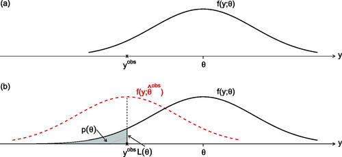
For simplicity we assume that $y=(y_1,\dots ,y_n)$ is a sample from a Normal with unit variance and unknown mean θ. The sample mean $\overline{y}$ is also Normal so that for all values of θ the pivot $z=n^{1/2}(\overline{y}-\theta )$) is standard Normal; and for further simplicity suppose that n = 1 and the observed $y=y^{\text{obs}}=10$; and that our theory seeks an assessment or testing of values for θ. In Figure 1(a), we record a typical density of the model and also the observed data value. In Figure 1(b), we record the amount of probability at the observed data point under some θ value and do so as a proportion of the maximum possible; this is designated $L(\theta )$ and is called the observed likelihood function; we also record $p(\theta )$ which is the probability to the left of the data point $y^{\text{obs}}$. Here, ${\widehat{\theta }}^{\text{obs}}$ is the value of the parameter that puts maximum probability density at the observed data point $y^{\text{obs}}$; we also indicate by the dotted curve the corresponding density function $f(y;{\widehat{\theta }}^{\text{obs}})$. This maximum likelihood density function happens to be of central interest for bootstrap calculations.

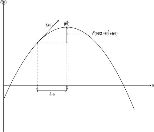
Fig. 1 The upper graph presents the model at some typical θ value and the observed data value $y^{\text{obs}}$; the lower graph records in addition the p-value and the likelihood for that θ value, and also in dots the density using the maximum likelihood $\theta ={\widehat{\theta }}^{\text{obs}}$ value for the parameter.

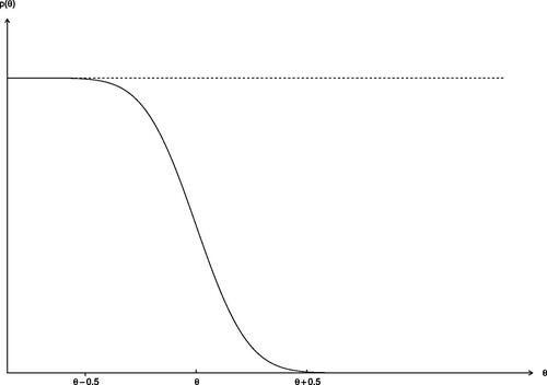
Now for general values of θ, we can record two items of information. The first is the normalized likelihood function$$L(\theta )=\hspace{0.17em}\text{exp}\hspace{0.17em}\left\{\ell \right(\theta \left)\right\}=\frac{f(y^{\text{obs}};\theta )}{f(y^{\text{obs}};{\widehat{\theta }}^{\text{obs}})}=c{f}^{\text{obs}}(\theta ).$$

The numerator is the observed value of the density function when the parameter is θ and tells us how much probability lies on that observed data point under θ; this is usually presented as a fraction of the maximum possible density at $y^{\text{obs}}$, obtained with $\theta ={\widehat{\theta }}^{\text{obs}}$. For the simple example, see Figures 1(b) and 2.

The second is the p-value function, which is less familiar than the likelihood but its value at any given parameter value is familiar as an ordinary p-value. For given data $y^{\text{obs}}$, the p-value function records the probability left of the data as a function of the parameter θ $$p(\theta )=F(y^{\text{obs}};\theta )=F^{\text{obs}}(\theta ).$$

See again Figure 2 for this simple Normal example. The p-value function simply records the usual left-sided p-value as a function of a general tested value θ. Thus, the p-value function is the observed value of the distribution function under θ: $p(\theta )=F(y^{\text{obs}};\theta )=F^{\text{obs}}(\theta )$. As such it records the percentile position of the data for any choice of scalar parameter value θ. Because this function is nonincreasing and $0\le p(\theta )\le 1$, we can regard $1-p(\theta )$, formally at least, as a cumulative distribution function for θ. The resulting distribution is in the spirit of Fisher’s fiducial distribution. As shown in Fraser (2017) and summarized in Section 5, this function is well defined and accurately approximated to the third order, for a wide range of applied problems with vector-valued y and scalar parameter of interest.

Fig. 2 The upper graph presents the p-value function and the lower graph the likelihood function, for the simple Normal example; the median estimate of θ is ${\widehat{\theta }}_{0.50}$ which here is the maximum likelihood value ${\widehat{\theta }}^{\text{obs}}=10$.

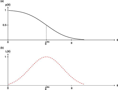
These items are what the data and model give us as the primary inference material; they are recorded for our present example in Figure 2(a,b). We recommend the use of these two key inference functions as the inference information.

For Example 1, consider some applications of the p-value function:

1. With an observed value $y=y^{\text{obs}}$ and for any hypothesized null value θ₀, the value of $p(\theta )$ at θ₀ is the one-sided p-value, and records the statistical position of the observed data.

2. The endpoint of a left-sided 97.5% confidence interval with data $y^{\text{obs}}=10$ is the value ${\widehat{\theta }}_{0.975}=p^{-1}(0.975)$ for which the p-value is 97.5%, that is, $\mathit{Pr}\{y\le 10;{\widehat{\theta }}_{0.975}\}=0.975$. As seen in Figure 3(a), take the value 0.975 on the vertical $p(\theta )$ axis, run a line horizontally to the p-value curve, and then down to the θ axis; this gives the value ${\widehat{\theta }}_{0.975}=p^{-1}(0.975)=8.04$, which is the lower 97.5% confidence bound, the value that in repetitions would be less than the true value 97.5% of the time. In the same way, ${\widehat{\theta }}_{0.025}=11.96$ is the endpoint of a left-sided 2.5% interval. Taken together the two percentiles give a 95% two-sided interval $({\widehat{\theta }}_{0.975},{\widehat{\theta }}_{0.025})=(8.04,11.96)$. We rely here on confidence intervals as derived by inverting an essential pivot, as distinct from intervals defined by shortest interval with given overall coverage probability. Thus, the 95% interval is the set of parameter values not rejected by either of the 2.5% single-tailed tests. For more on the two different approaches to intervals and the role of conditional inference, together with examples, see Fraser, Reid, and Lin (2018).

3. Similarly, for the 50% point for which $p(\theta )=0.50,{\widehat{\theta }}_{0.50}$ is the median estimate for θ. First, locate 0.5 on the vertical axis and across to the curve. Then, drop down to the horizontal axis to get the value ${\widehat{\theta }}_{0.50}=10$.

4. For any given test size α, the inverse function $p^{-1}(\alpha )$ gives the corresponding parameter value say θ₀ that is being tested with the observed data value as critical point. Although the view taken here argues against fixed-level testing, there are occasions where the notions of size and power can be convenient. To find the value θ₀ being tested at level α relative to the observed data as critical point locate the particular value of α on the vertical axis, then read across to the p-value curve, and then down to the θ₀ for testing.

5. For the size α test with the data point as critical value, the p-value function gives the power of that test at any other parameter value θ; this is conditional power given model information identified from the data, but as such it is also marginal power: the power at θ is $p(\theta )$. First be aware of the critical value for the test of size α as given in (4). Then for any other value of θ the probability that the α-level test rejects the null hypothesis is $p=\text{Pr}\{y\le y^{\text{obs}};\theta \}=p(\theta )$, which is, the value of the p-value function at θ. Perhaps more importantly the p-value function describe the sensitivity of the procedure in distinguishing parameter values in the broad range around the maximum likelihood value.

6. In addition, if for some value on the θ axis, say θ = 8, we found that the corresponding p-value was large or very large we would infer that the true value was large or much larger than the selected value 8. And similarly if the p-value was small or very small, say at θ = 12 we would infer that the true value was small or much smaller than the selected 12. Thus, the observed p-value function not only shows extremes among θ values but also the direction in which such extremes occur; it thus provides inference information widely for different users who might have concern for different directions of departure.

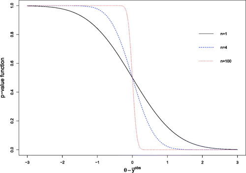
7. Based on the properties above, it follows that the location and shape of the p-value function provides a clear way to assess the evidence about the parameter θ. Figure 4 shows three p-value functions corresponding to $n=1,n=4,\text{and}n=100$.

8. The p-value function is central to a widely available approach to inference based on approximate conditioning, as discussed in Sections 4 and 5. When a complete sufficient statistic is available, the present approach coincides with the usual inferences based on sufficiency. When a reduction by sufficiency is not available as is all too frequently the case, the present approach is widely available and gives an accurate approximation to a well defined p-value function; and as illustrated in Section 5 is immediately available. The theory uses conditioning derived from model continuity. The Normal location problem of this section was chosen as extremely simple, partly to keep technical details to a minimum, and partly to emphasize that the general case is as simple but with slightly less familiar computation. The next three sections show how the ideas of the p-value function for a single, scalar parameters are available quite generally for models with multi-dimensional parameters that have no reduction via a sufficient statistic. And as the next section shows it is often the case that for problems of genuine scientific interest, it is reasonable to focus attention on a single parameter of interest and the present p-value function.

Fig. 3 The upper graph (a) indicates the median estimate and the one-sided 0.975 and 0.025 confidence bounds; the lower graph (b) records the observed likelihood function.

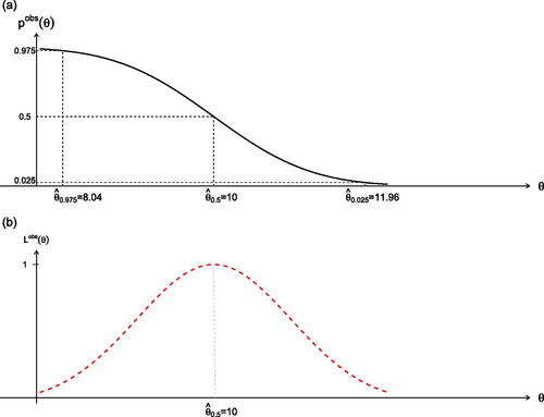
Fig. 4 The p-value function for n = 1 (solid), n = 4 (dashed), n = 100 (dotted).

3 Narrowing the Focus to the Essential Parameter: Three Illustrations From Science

The examples in this section are here to illustrate three instances where scientific problems of considerable import lend themselves to an analysis that puts focus on a scalar parameter of interest and a related scalar variable. These examples discuss such a parameter of interest, but we wait until later sections to address the role of nuisance parameters and the reduction of data observations to a single dimension.

3.1 Trajectory of Light

A theory being floated in the early part of the last century indicated that the trajectory of light would be altered in the presence of a large mass like the sun. An opportunity arose in 1919 when the path of an anticipated total eclipse was expected to transit portions of Africa. During the eclipse an expedition was able to measure the displacement of light from a star in the Hyades cluster whose light would pass very close to the sun, and whose position relative to nearby visible stars was then seen to be displaced, by an amount indicated by the theory. This was an observational study but in many details duplicated aspects of an experiment. In this example, the intrinsic variable relevant to the theory was the displacement on the celestial sphere of the prominent star relative to others whose light trajectory was at some greater distance from the sun, and was calculated away from the sun.

3.2 Search for the Higgs Boson

In 1994, Abe (1994) and coauthors reported on the search for the top quark. High energy physicists were using the collider detector at Fermilab to see if a new particle was generated in certain particle collisions. Particle counts were made in time intervals with and without the collision conditions; in its simplest form this involves a Poisson variable y and parameter θ, and whether the Poisson parameter is shifted to the right from a background radiation level θ₀, thus increased under the experimental intervention. This is an experimental study and such typically provide more support than an observational study.

The statistical aspects of the problem led to related research, for example, Fraser, Reid, and Wong (2004), and to a collaborative workshop with statisticians and high energy physicists (Banff International Research Station 2006). This in turn led to an extensive simulation experiment launched by the high energy physicists, in preparation for the CERN investigation for the Higgs boson. The p-value function approach to this problem is detailed in Davison and Sartori (2008), with the measure of departure recommended in Fraser, Reid, and Wong (2004), and shown to give excellent coverage for the resulting confidence intervals. The p-value reached in the CERN investigation was 1 in 3.5 million, somewhat different from the widely used 5%.

3.3 Human–Computer Interaction

A researcher in human–computer interaction (HCI) is investigating improvements to the interface for a particular popular computer software package. The intrinsic variable could, for example, be the reduction in learning time under the new interface, or a qualitative evaluation of the ease of learning. In this experimental investigation, advice is sought on the appropriate model and appropriate approximation for the distribution of the intrinsic variable.

3.4 Overview

In each of these examples, the methodology for the Normal example in Section 2 is immediately available and follows methods described in Fraser (2017). The resulting p-value and likelihood functions are readily computed, and inference is then of the same type as that in the simple example but computational details differ. Extensions from this are also available for testing vector parameters and use recently developed directional tests (Sartori, Fraser, and Reid 2016). The next two sections discuss the conditioning and then the use of the approximations.

4 Conditioning for Accurate Statistical Inference

Fisher (1930) introduced the notion of an ancillary statistic, to formalize the use of conditioning for inference based on features of the observed data. An ancillary statistic is a function of the data whose distribution does not depend on the parameter or parameters in the model for the observed response. As a simple example, if the sample size n in an investigation is random, rather than fixed, but its distribution does not depend on the parameters governing the model for the response y, then the appropriate model for inference is $f(y|n;\theta )$, not $f(y,n;\theta ,\varphi )=f(y|n;\theta )f(n;\varphi )$, where $\varphi$ might be present as a parameter for the distribution for n. The weighing machine example in Cox (1958) is another example of an obvious conditioning; in this case a random choice is made between a precise measurement of y and an imprecise measurement, and the resulting inference based on y should be conditional on this choice.

Example 2. A

pair of uniformly distributed variables

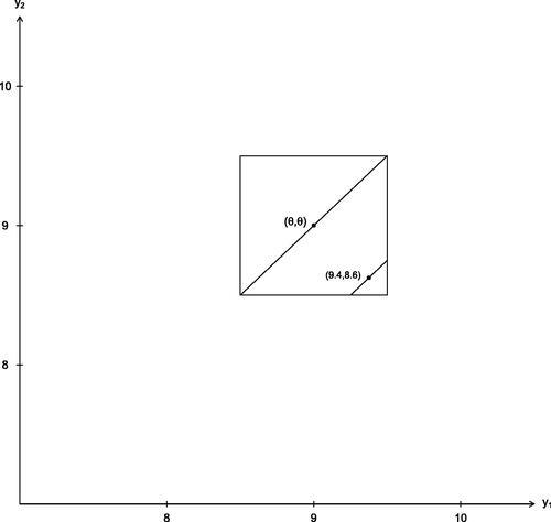
Consider a response y that is uniformly distributed on the interval $(\theta -1/2,\theta +1/2)$ and suppose we have a sample of n = 2 with data $(9.4,8.6)$, Figure 5 presents the sample space for some θ value with observed data $(9.4,8.6)$; the actual sample space indicated is that for $\theta ={\widehat{\theta }}^{\text{obs}}=9$ which is just ${\overline{y}}^{\text{obs}}$.

Fig. 5 The sample space for a sample of 2 from the uniform distribution on $(\theta -1/2,\theta +1/2)$. The observed data point is $(9.4,8.6)$; the square is the sample space for $\theta ={\widehat{\theta }}^{\text{obs}}={\overline{y}}^{\text{obs}}=9$. Only θ-values in the range 8.9–9.1 can put positive density at the observed data point. The short line through this point illustrates the small data range consistent with the observed data.

A quick conventional approach might use approximate normality and the pivot $t=(\overline{y}-\theta )/2^{-1/2}{(1/12)}^{1/2}$, where the denominator is the standard deviation 0.20 of the sample mean. Figure 6 shows for some θ value the corresponding distribution of $\overline{y}$ with its standard deviation 0.20. The corresponding p-value function $\Phi \{(9-\theta )/0.20\}$ from the data is plotted in Figure 7. This provides an approximate 95% interval for θ as $(9-1.96·0.20,9+1.96·0.20)=(8.61,9.39)$, but not all is well.

Fig. 6 The approximate density of $\overline{y}$ for some θ value.

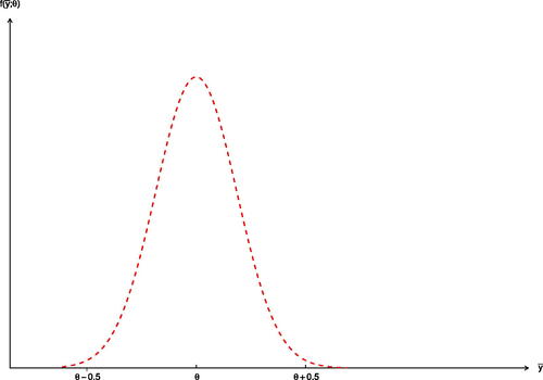
Fig. 7 The observed p-value function from the approximate pivot $t=({\overline{y}}^{\text{obs}}-\theta )/2^{-1/2}{(1/12)}^{1/2}=0.20({\overline{y}}^{\text{obs}}-\theta )$ as a function of θ.

In Figure 5, we show the sample space centered at θ, and indicate the line parallel to the 1-vector through the data point $(9.4,8.6)$, and related lines would be parallel to this. Suppose we think of changing the θ value: the corresponding square domain will shift to the lower left or to the upper right, but only θ-values from 8.9 to 9.1 can put positive density at the observed data point $(9.4,8.6)$. The short line through the observed data point records the corresponding range and the parameter can only be at most 0.1 from the data. Any statistic describing these diagonal lines has a distribution that cannot depend on θ and is thus ancillary. The conditional model on the line through the data point is $U(\theta -0.1,\theta +0.1)$ with half-range 0.1: the parameter can be at most 0.1 from the data and the data can only be at most 0.1 from the parameter. An exact 95% confidence interval for θ is $(9-0.095,9+0.095)=(8.905,9.095)$, which is radically different from the approximate result $(8.61,9.39)$ in the preceding paragraph.

Indeed, the initial confidence interval includes θ values that are not possible, and also those for which the actual coverage is 100%. Of course, the first interval uses an extreme approximation but conditioning on $y_1-y_2$ makes clear how the observed data restricts the range of possible parameter values. In Figure 8, we record the exact observed likelihood function from the data $(9.4,8.6)$; it shows the range of possible values for θ and demonstrates the restrictions on the parameter.

Fig. 8 The exact observed a likelihood function from the data $(9.4,8.6)$.

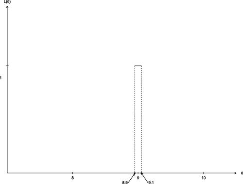
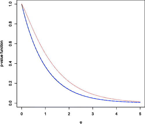
Fig. 9 For the simple exponential model, the p-value function is plotted using the Normal approximation for r (dotted), using the third-order approximation (dashed), and compared to the exact p-value function (solid).

In many cases for statistical inference, there is not such an obvious function of the data that is exactly distribution constant, However, there are many models in which there is an essentially unique quantile function or data-generating function $y_i=y(\theta ,z_i)$, where the distribution of z is known. For example, if y_i follows a location model with density $f(y_i-\theta )$, we can write $y_i=\theta +z_i$, with the distribution of z_i known to be $f(·)$. Similarly with independent sampling from a normal model with $E(y_i)=x_i^{\prime }\beta$ and $\text{var}(y_i)={\sigma }^2$, the model can be written $y_i=x_i^{\prime }\beta +\sigma z_i$, with z_i following a N(0, 1) distribution.

This quantile function provides the information needed to construct conditional inference, by examining how parameter change affects variable change for fixed quantile. This is summarized by the n × p matrix of derivatives$$V=(v_1,\dots ,v_p)=\frac{\partial y}{\partial \theta }{|}_{\text{fixed} \text{pivot} z}$$evaluated at the data $y^{\text{obs}}$ and maximum likelihood estimate ${\widehat{\theta }}^{\text{obs}}$. The p vectors $v_1,\dots ,v_p$ are tangent to the contours of an approximate ancillary statistic, and the model conditional on these contours can be expressed in exponential family form. Recent asymptotic theory as summarized in Fraser (2017) shows that this conditional model provides a third-order inference information with extremely simple methods of analysis. If the given model happens to be a normal location model, then this will also reproduce the simple analysis above.

In Example 2, the quantile expression of the model is $y_i=\theta +u_i$, where u_i follows a $U(-1/2,1/2)$ distribution. The 2 × 1 matrix V is simply $(1,1)\prime$, and this defines the sloped lines in the sample space in Figure 5.

In the linear regression model, the matrix V is $n\times (p+1)$, where p is the dimension of β. The leading n × p submatrix is simply X with ith row $x_i^{\prime }$, and the final column of V is the observed standardized residual vector $({\widehat{z}}_1,\dots ,{\widehat{z}}_n)$.

Example 3.

Ratio of Normal variables

This example has appeared widely in the literature and is often called the Fieller (1954)- Creasy (1954) problem. In its simplest form, we have two Normal variables with common variance, and we are interested in the ratio $\psi ={\mu }_1/{\mu }_2$ of their means; a nearly equivalent parameter is the direction $\psi =\alpha$ of the vector mean $({\mu }_1,{\mu }_2)$ as an angle, say negative, from the positive μ₁ axis. The problem also has close connections to regression calibration methods. Various routes to conditioning have been discussed in the past. Fraser, Reid, and Lin (2018) examine the model from the present viewpoint, but we do not attempt to reproduce the discussion here; other related examples are also examined there.

The next section outlines the automatic conditioning based on model continuity: this is preliminary to the widely available accurate approximations for the p-value function. We also outline the route to the accurate p-value function approximations.

5 Accurate p-value Functions

Two main features make the p-value function central to inference. The first of these is its multiple uses, as set out in Section 2. The second is the broad availability of an asymptotic approximation to the p-value function. This approximation is uniquely determined to third order and is conditional on an approximately ancillary statistic. The matrix V described in Section 4 enables construction of an approximating exponential family model but avoids explicit construction of the approximately ancillary statistic. This exponential model provides a route to inference for a scalar parameter of interest that is accurate to third order, that is, the inference approximation errors are $O(n^{-3/2})$. We illustrate this approximation route in this section; details on the construction of the tangent exponential model, if needed, are provided in Fraser (2017).

Example 4.

Exponential life model

As a simple and transparent example consider the exponential life model $f=\hspace{0.17em}\text{exp}\hspace{0.17em}\{-\phi y+\hspace{0.17em}\text{log}\hspace{0.17em}\phi \}$ with failure rate $\phi$ and observed life y, both on the positive axis; and for data, take $y^{\text{obs}}=1$ with little loss of generality. Note that increasing $\phi$ corresponds to decreasing life y. The observed likelihood function is $\ell (\phi )=-\phi +\hspace{0.17em}\text{log}\hspace{0.17em}\phi$ and the maximum likelihood estimate is $\widehat{\phi }=1/y^{\text{obs}}=1$. An approximate p-value function for $\phi$ can be obtained from standard asymptotic theory, for example, using the standardized maximum likelihood estimate $q=\widehat{\phi }-\phi$ we have $p(\phi )$ approximated by $\Phi (q)$, where $\Phi$ is the standard normal cdf. The signed square root of the log-likelihood ratio statistic also follows a normal distribution in the limit, so another approximate p-value function is $p_L(\phi )=\Phi (r)$, where $r=\text{sign}(\widehat{\phi }-\phi ){\{2(\phi -\widehat{\phi }-\hspace{0.17em}\text{log}\hspace{0.17em}\phi )\}}^{1/2}$. As described below, the saddlepoint approximation leads to a pivotal quantity $r^{*}=r+r^{-1}\hspace{0.17em}\text{log}\hspace{0.17em}(q/r)$ that follows the standard normal distribution to third order. The approximations $p_L(\phi )$ and $p_{3rd}(\phi )=\Phi (r^{*})$ are compared to the exact p-value function $p_{\mathit{Exact}}(\phi )=\hspace{0.17em}\text{exp}\hspace{0.17em}\{-\phi \}$ in Figure 10. Although n = 1, the third-order approximation is extremely accurate.

Fig. 10 A log-likelihood function with the log-likelihood ratio $r^2/2$ and the standardized maximum likelihood departure $q=(\phi -\widehat{\phi }){\mathcal{J}}_{\phi \phi }^{1/2}$ identified.

The steps in obtaining this approximation are as follows:

1. The exponential model

   Exponential models have a simple form as an exponential tilt of some initial density h(s)(1) $$f(s;\phi )=\hspace{0.17em}\text{exp}\hspace{0.17em}\{\phi \prime s-\kappa (\phi \left)\right\}h\left(s\right),$$(1) where the p-dimensional variable $s=s(y)$ and parameter $\phi =\phi (\theta )$ are called canonical and can in turn be functions of some background variable y and parameter θ.

2. Saddlepoint accuracy

   The saddlepoint approximation came early to statistics (Daniels 1954) but only more recently has its power for analysis been recognized. The saddlepoint approximation to the density of s can be expressed in terms of familiar likelihood characteristics; in particular, the log-likelihood ratio $r^2/2=\ell (\widehat{\theta };y)-\ell (\theta ;y)$ and the standardized maximum likelihood departure $q=(\phi -\widehat{\phi }){\mathcal{J}}_{\phi \phi }^{1/2}$, with the latter calculated in the canonical parameterization. These measures are illustrated in Figure 10. The saddlepoint approximation has the form(2) $$f(s;\phi )\mathit{ds}=\frac{\hspace{0.17em}\text{exp}\hspace{0.17em}(k/n)}{{(2\pi )}^{1/2}}\text{exp}\hspace{0.17em}(-r^2/2)\frac{r}{q}dr$$(2) using the just defined familiar statistical quantities r and q.

3. Accurate p-value approximation

   If p = 1, then the distribution function can be computed from (2) by noting that $\mathit{rdr}=(\widehat{\phi }-\phi )\mathit{ds}$ and then integrating by parts, leading to the Barndorff-Nielsen (1983) formula for the p-value function(3) $$p(\phi )=\Phi \{r+r^{-1}\hspace{0.17em}\text{log}\hspace{0.17em}(q/r\left)\right\}=\Phi \left(r^{*}\right),$$(3) still in terms of the simple r and q statistical quantities. This was used above for the exponential life model.

4. With a nuisance parameter

   Suppose in (1) that the parameter of interest ψ is a component of $\phi$, with the remaining components λ, say treated as nuisance parameters. A relatively simple adjustment to $r^{*}$ above can be used to compute an accurate approximation to the p-value function for ψ. The arguments use the general theory of conditioning in Section 4, followed by a Laplace approximation for the required integration. The result is an approximation to $p(\psi )$ given by (3) but with r computed from the profile log-likelihood function: $r^2/2=\ell (\widehat{\phi };s)-\ell ({\widehat{\phi }}_{\psi };s)$ and q replaced by(4) $$Q=q{\left(\frac{\left|{\widehat{\mathcal{J}}}_{\lambda \lambda }\right|}{\left|{\widehat{\mathcal{J}}}_{\lambda \lambda }\right|}\right)}^{-1/2},$$(4) where $q=(\widehat{\psi }-\psi ){\mathcal{J}}_p{(\widehat{\psi })}^{1/2}$ is the standardized maximum likelihood departure as before, ${\mathcal{J}}_p=-{\mathcal{l}}_p\prime \prime (\psi )$ is the observed information in the profile log-likelihood function, and ${\mathcal{J}}_{\lambda \lambda }$ is the nuisance parameter submatrix of the full observed information matrix, evaluated in the numerator at the constrained maximum likelihood estimate ${\widehat{\phi }}_{\psi }$, and evaluated in the denominator at the full maximum likelihood estimate $\widehat{\phi }$.

   Often the parameter of interest is a nonlinear function of the canonical parameter, which we write $\psi (\phi )$, and the nuisance parameter $\lambda =\lambda (\phi )$. The arguments leading to (3) can be developed by building on the conditioning of Section 4 and the Laplace integration mentioned above, and the result is an approximation to the p-value function again given by (3), but with q replaced by a quantity similar to Q in (4)(5) $$Q=\tilde{q}{\left(\frac{\left|{\widehat{\mathcal{J}}}_{(\lambda \lambda )}\right|}{\left|{\widehat{\mathcal{J}}}_{(\lambda \lambda )}\right|}\right)}^{-1/2},$$(5) where the notation ${\mathcal{J}}_{(\lambda \lambda )}$ means that λ is re-expressed in terms of a nuisance parameterization that accommodates the non-linearity in the dependence of the parameter of interest on the canonical parameter of the exponential model. The quantity $\tilde{q}$ is a standardized maximum likelihood departure, as above, but in a parameterization that takes account of the nonlinearity of ψ as a function of $\phi$; see, for example, Fraser, Reid, and Wu (1999).

   In the next section we give an example of the approximation of the p-value function in this setting.

5. General parametric model for y

If the statistical model of interest is not an exponential model, then a preliminary step based on Section 4 is used to construct what we have called the tangent exponential model, which implements conditioning on an approximate ancillary statistic using the matrix V. The canonical parameter of the tangent exponential model is $\phi (\theta )=\partial \ell (\theta ;y)/\partial V$. It can be shown that this approximation is sufficient to obtain an approximate p-value function to third order, and the steps are essentially the same as those for an exponential model described above. The argument is summarized in Reid and Fraser (2010) and Fraser, Reid, and Wu (1999).

One feature of these third-order approximations is that the pivotal quantity used to generate the p-value function is determined at the same time as its distribution is approximated, an astonishing result!

6 Applications

Many examples are available in the literature; see, for example, Fraser, Wong, and Wu (2004) and Fraser, Reid, and Wong (2009) and the book by Brazzale, Davison, and Reid (2007).

Example 5.

Mean of a gamma density

As an illustration of the formulas in the previous section, we now consider the analysis of the lifetime data in Gross and Clark (1975) using a gamma model. The observations are (152, 152, 115, 109, 137, 88, 94, 77, 160, 165, 125, 40, 128, 123, 136, 101, 62, 153, 83, 69) being 20 survival times for mice exposed to 240 rads of gamma radiation. The gamma exponential model for a sample $(y_1,\dots ,y_n)$ is$$f(y;\alpha ,\beta )\Pi d{y}_i={\Gamma }^{-n}(\alpha ){\beta }^{n\alpha }\hspace{0.17em}\text{exp}\hspace{0.17em}\{\alpha s_1-\beta s_2\}{(\Pi y_i)}^{-1}\Pi d{y}_i,$$where $(s_1,s_2)=(\Sigma \hspace{0.17em}\text{log}\hspace{0.17em}{y}_i,\Sigma y_i)$ records the canonical variable and $(\alpha ,\beta )$ records the canonical parameter. Inference for α or β would use (4) for Q in approximation (3); and now we illustrate inference for the mean $\mu =\alpha /\beta$, a nonlinear function of the canonical parameter.

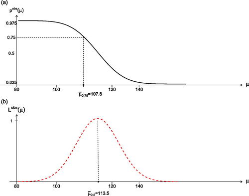
Grice and Bain (1980) considered such inference for the mean and eliminated the remaining nuisance parameter by “plugging in” the nuisance parameter estimate and then using simulations to adjust for the plug-in approach. Fraser, Reid, and Wong (1997) investigated the use of $r_{\mu }^{*}$ based on (5) and verified its accuracy; the results for the Gross and Clark (1975) data are recorded in Figure 11. For example, the 75% lower confidence bound is 107.8 which tells us that the given data provide 75% confidence that the true μ is in the interval $(107.8,\infty )$. Any one-sided or two-sided confidence interval is thus available immediately from the p-value graph.

Fig. 11 The p-value function and log-likelihood function for the mean of the Gamma model data from Gross and Clark (1975).

Example 6

: Model selection: Box and Cox

Location-scale and regression models have an important role in applications. Instances, however, do arise where the investigator is unsure of the mode of expression for his primary variable: Should he make a transformation of some initial variable, say a log or power transformation? Or should he take a family of such transformations and thus have a spectrum of regression models? A common concern is whether curvature should be applied to an initial response variable to achieve the linearity expected for a regression model. Box and Cox (1964) proposed a likelihood analysis, and a Bayesian modification. We consider here the present p-value function approach.

The regression model with the power transformation can be written as $y^{\lambda }=X\beta +e$ where e is a vector of say Normal $(0,{\sigma }^2)$ errors. For our notation, it seems preferable to write it as$$y={(X\beta +e)}^{1/\lambda },$$where the power is applied coordinate by coordinate and the data and model coordinates are assumed to be positive. The power or curvature parameter λ is typically the primary parameter; while the regression parameters β only have physical meaning relative to a particular choice of the transformation parameter value λ. The third-order analysis is discussed in Fraser, Wong, and Sun (2009) using an example from Chen, Lockhart, and Stephens (2002). The resulting p-value function for the parameter λ is recorded there as Figure 1(e) on page 12, and the 95% central confidence interval for λ is $(0.694,2.378)$ on page 14. This shows that it is extremely hard to pin down possible curvature even with the large sample size n = 107; linearity corresponds to λ = 1.

Example 7

: Extreme value model

The extreme value model has immediate applicability to the modeling of extremes, say for the largest or smallest, in a sample or sequence of available data values, perhaps collected over time or space; it is of particular importance for the study say of climate extremes and has generalizations in the form of the Weibull model. The model has the density form$$f(y;\theta )=\hspace{0.17em}\text{exp}\hspace{0.17em}\{-(y-\theta )-e^{-(y-\theta )}\}.$$

For our purposes here, it provides a very simple example where the likelihood and the p-value functions are immediately available, in exact and in the third-order form. Suppose we have a single data value $y^{\text{obs}}=21.5$ as discussed in Fraser, Reid, and Wong (2009). The log-likelihood and p-value functions have the simple form$$\ell (\theta )=\theta -e^{\theta -21.5}, p(\theta )=\hspace{0.17em}\text{exp}\hspace{0.17em}(-e^{\theta -21.5}).$$

For the third-order approximation, we have r and q as the signed likelihood ratio and the Wald departure$$r=\text{sign}(\widehat{\theta }-\theta )[2{\left\{\ell \right(\widehat{\theta }-\ell (\theta )\left\}\right]}^{1/2}, q=\text{sign}(\widehat{\theta }-\theta \left)\right|\widehat{\phi }-\phi |{\widehat{\mathcal{J}}}_{\phi \phi }^{1/2}$$where the exponential parameterization $\phi (\theta )=\hspace{0.17em}\text{exp}\hspace{0.17em}(\theta -21.5)-1$ is obtained by differentiating $\ell (\theta ;y)$ with respect to y where the V from Section 4 is just a one-by-one “matrix” given as V = 1. The likelihood and p-value function are plotted on page 4 of Fraser, Reid, and Wong (2009); in particular, the plot of the p-value function also records the third-order approximation we have been recommending; it is recorded as a dotted curve that is essentially indistinguishable from the exact as a solid curve. And of course any confidence interval or bound is immediately available.

Example 8

: Logistic regression and inference for discrete data

Discrete data, often frequency data such as with the binomial, two by two tables, contingency tables, Poisson data, and logistic regression are commonly analyzed by area specific methods and some times by likelihood methods. Davison, Fraser, and Reid (2006) examine such discrete data analyses and demonstrate the straightforward steps and accuracy available for such problems, using the present p-value function approach and the related third-order accurate approximations; the discreteness, however, does lower the effective accuracy to second order. The general methods are also discussed there together with the minor modifications required for the discreteness. Binary regression is discussed in detail and the data from Brown (1980) on 53 persons with prostate cancer is analyzed. The methods are also applied to Poisson counts and illustrated with data on smoking and lung cancer deaths (Frome 1983).

7 Discussion

The p-value function reports immediately: if the p-value function examined at some parameter value is high or very high as on the left side of the graph, then the indicated true value is large or much larger than that examined; and if the p-value function examined at some value is low or very low as on the right side of the graph, then the indicated true value is small or much smaller than that examined. The full p-value function arguably records the full measurement information that a user should be entitled to know!

We also note that the p-value function is widely available for any scalar interest parameter and any model-data combination with just moderate regularity, and has available computational procedures.

In addition to the overt statistical position, the p-value function also provides easily and accurately many of the familiar types of summary information: a median estimate of the parameter; a one-sided test statistic for a scalar parameter value at any chosen level; the related power function; a lower confidence bound at any level; an upper confidence bound at any level; and confidence intervals with chosen upper and lower confidence limits. The p-value reports all the common inference material, but with high accuracy, basic uniqueness, and wide generality.

From a scientific perspective, the likelihood function and p-value function provide the basis for scientific judgments by an investigator, and by other investigators who might have interest. It thus replaces a blunt yes or no decision by an opportunity for appropriate informed judgment. In the high energy physics examples very small p-values are widely viewed as evidence of a discovery: Abe (1994) obtained p = 0.0026, and the LHC collaboration obtained 1 in 3.5-million before they were prepared to claim discovery. This is not a case of statisticians choosing a decision break point for others; but rather the provision of full inference information for others to make judgments. The responsibility for decisions made on the basis of inference information would rest elsewhere.

Acknowledgments

Sincere thanks to the Editor and Associate Editor for extraordinarily helpful suggestions and proposed content; we feel very deep appreciation. And deep thanks to Nancy Reid for counsel and deep insight. And special thanks to Wei Lin for preparing the graphs and for assistance with the manuscript preparation, to Mylène Bédard for calculations and simulations for the gamma mean problem, to Augustine Wong for assistance with examples.

Additional information

Funding

The author gratefully acknowledge support from the Natural Sciences and Engineering Research Council of Canada and The Senior Scholars Fund at York University.

References

- Abe, F. (1994), “Evidence for Top Quark Production in pøp Collisions at Ãs =1.8 tev,” Physics Review Letters, 69, 033002.
- Banff International Research Station (2006), “Statistical Inference Problems in High Energy Physics and Astronomy,” available at https://www.birs.ca/events/2006/5-day-workshops/06w5054.
- Barndorff-Nielsen, O. E. (1983), “On a Formula for the Distribution of the Maximum Likelihood Estimate,” Biometrika, 70, 343–365. DOI: 10.1093/biomet/70.2.343.
- Box, G., and Cox, D. (1964), “An Analysis of Transformations” (with discussions), Journal of Royal Statistical Society, Series B, 26, 211–252. DOI: 10.1111/j.2517-6161.1964.tb00553.x.
- Brazzale, A. R., Davison, A. C., and Reid, N. (2007). Applied Asymptotics Case Studies in Small-Sample Statistics, Cambridge, UK: Cambridge University Press.
- Brown, B. (1980), “Prediction Analysis for Binary Data,” in Biostatistics Casebook, eds. B. W. B. R. G. Miller, B. Efron, and L. E. Moses, New York: Wiley, pp. 3–18.
- Chen, G., Lockhart, R., and Stephens, M. (2002), “Box–Cox Transformations in Linear Models: Large Sample Theory and Tests of Normality,” Canadian Journal of Statistics, 30, 177–234. DOI: 10.2307/3315946.
- Cox, D. R. (1958), “So+-me Problems Connected With Statistical Inference,” Annals of Mathematical Statistics, 29, 357–372. DOI: 10.1214/aoms/1177706618.
- Creasy, M. (1954), “Limits for the Ratios of Means,” Journal of Royal Statistical Society B, 16, 186–194. DOI: 10.1111/j.2517-6161.1954.tb00160.x.
- Daniels, H. E. (1954), “Saddlepoint Approximations in Statistics,” Annals of Mathematical Statistics, 46, 21–31.
- Davison, A., Fraser, D., and Reid, N. (2006), “Improved Likelihood Inference for Discrete Data,” Journal of Royal Statistical Society, Series B, 68, 495–508. DOI: 10.1111/j.1467-9868.2006.00548.x.
- Davison, A. C., and Sartori, N. (2008), “The Banff Challenge: Statistical Detection of a Noisy Signal,” Statistical Science, 23, 354–364. DOI: 10.1214/08-STS260.
- Fieller, E. (1954), “Some Problems in Interval Estimation,” Journal of Royal Statistical Society, Series B, 16, 175–185. DOI: 10.1111/j.2517-6161.1954.tb00159.x.
- Fisher, R. (1922), “On the Mathematical Foundations of Theoretical Statistics,” Philosophical Transaction of Royal Society A, 222, 309–368. DOI: 10.1098/rsta.1922.0009.
- Fisher, R. (1930), “Inverse Probability,” Proceedings of the Cambridge Philosophical Society, 26, 528–535. DOI: 10.1017/S0305004100016297.
- Fraser, D., Reid, N., and Lin, W. (2018), “When Should Modes of Inference Disagree? Some Simple But Challenging Examples,” Annals of Applied Statistics, 12, 750–770. DOI: 10.1214/18-AOAS1160SF.
- Fraser, D., Wong, A., and Sun, Y. (2009), “Three Enigmatic Examples and Inference From Likelihood,” Canadian Journal of Statistics, 37, 161–181. DOI: 10.1002/cjs.10008.
- Fraser, D., Wong, A., and Wu, J. (2004), “Simple Accurate and Unique: The Methods of Modern Likelihood Theory,” Pakistan Journal of Statistics, 20, 173–192.
- Fraser, D. A. S. (2017), “The p-value Function: The Core Concept of Modern Statistical Inference,” Annual Review of Statistics and its Application, 4, 153–165. DOI: 10.1146/annurev-statistics-060116-054139.
- Fraser, D. A. S., Reid, N., and Wong, A. (1997), “Simple and Accurate Inference for the Mean of the Gamma Model,” Canadian Journal of Statistics, 25, 91–99. DOI: 10.2307/3315359.
- Fraser, D. A. S., Reid, N., and Wong, A. (2004), “On Inference for Bounded Parameters,” Physics Review D, 69, 033002.
- Fraser, D. A. S., Reid, N., and Wong, A. (2009), “What a Model With Data Says About Theta,” International Journal of Statistical Science, 3, 163–177.
- Fraser, D. A. S., Reid, N., and Wu, J. (1999), “A Simple General Formula for Tail Probabilities for Frequentist and Bayesian Inference,” Biometrika, 86, 249–264. DOI: 10.1093/biomet/86.2.249.
- Frome, E. L. (1983), “The Analysis of Rates Using Poisson Regression Models,” Biometrics, 39, 665–674. DOI: 10.2307/2531094.
- Grice, J., and Bain, L. (1980), “Inference Concerning the Mean of the Gamma Distribution,” Journal of American Statistical Association., 75, 929–933. DOI: 10.1080/01621459.1980.10477574.
- Gross, A., and Clark, V. (1975), Survival Distributions: Reli-ability Applications in the Biomedical Sciences. New York: Wiley.
- Neyman, J., and Pearson, E. S. (1933), “On the Problem of the Most Efficient Tests of Statistical Hypotheses,” Philosophical Transaction of Royal Society A, 231, 694–706.
- Reid, N., and Fraser, D. A. S. (2010), “Mean Likelihood and Higher Order Approximations,” Biometrika, 97, 159–170. DOI: 10.1093/biomet/asq001.
- Rozeboom, W. (1960), “The Fallacy of the Null-Hypothesis Significance Test,” Psychological Bulletin, 57, 416–428.
- Sartori, N., Fraser, D., and Reid, N. (2016), “Accurate Directional Inference for Vector Parameters,” Biometrika, 103, 625–639. DOI: 10.1093/biomet/asw022.
- Sterling, T. D. (1959), “Publication Decisions and Their Possible Effects on Inferences Drawn From Tests of Significance—or Vice Versa,” Journal of American Statistical Association, 54, 30–34. DOI: 10.2307/2282137.
- Wasserstein, R., and Lazar, N. (2016), “The ASA’s Statement on p-values: Context, Process, and Purpose,” The American Statistician, 70, 129–133. DOI: 10.1080/00031305.2016.1154108.