A Proposed Hybrid Effect Size Plus p-Value Criterion: Empirical Evidence Supporting its Use

ABSTRACT

When the editors of Basic and Applied Social Psychology effectively banned the use of null hypothesis significance testing (NHST) from articles published in their journal, it set off a fire-storm of discussions both supporting the decision and defending the utility of NHST in scientific research. At the heart of NHST is the p-value which is the probability of obtaining an effect equal to or more extreme than the one observed in the sample data, given the null hypothesis and other model assumptions. Although this is conceptually different from the probability of the null hypothesis being true, given the sample, p-values nonetheless can provide evidential information, toward making an inference about a parameter. Applying a 10,000-case simulation described in this article, the authors found that p-values’ inferential signals to either reject or not reject a null hypothesis about the mean (α = 0.05) were consistent for almost 70% of the cases with the parameter’s true location for the sampled-from population. Success increases if a hybrid decision criterion, minimum effect size plus p-value (MESP), is used. Here, rejecting the null also requires the difference of the observed statistic from the exact null to be meaningfully large or practically significant, in the researcher’s judgment and experience. The simulation compares performances of several methods: from p-value and/or effect size-based, to confidence-interval based, under various conditions of true location of the mean, test power, and comparative sizes of the meaningful distance and population variability. For any inference procedure that outputs a binary indicator, like flagging whether a p-value is significant, the output of one single experiment is not sufficient evidence for a definitive conclusion. Yet, if a tool like MESP generates a relatively reliable signal and is used knowledgeably as part of a research process, it can provide useful information.

KEYWORDS:

• NHST
• Minimum effect size plus p-value criterion
• MESP
• statistical evidence
• meaningful distance
• true power
• true Type I error rate

1 Introduction

There has been ongoing discussion of the use and misuse of p-values ever since R.A Fisher introduced the concept in Statistical Methods for Research Workers (Fisher 1925). However, in February 2015, it seemed a line had been drawn in the sand when the editors of Basic and Applied Social Psychology (BASP) effectively banned the use of null hypothesis significance testing (NHST) in manuscripts submitted for publication (Trafimow and Marks 2015). Blogging websites lit up as the news was spread; some met it with fanfare (Siegfried 2015; Woolston 2015), while others stoically attempted to defend NHST’s continued use (Nuzzo 2015; Leek and Peng 2015), albeit with the understanding that p-values alone are not adequate and are prone to misuses.

In March 2016, the American Statistical Association released a policy statement on p-values outlining their context, the process by which they should be used and their purpose in scientific literature and research (Wasserstein and Lazar 2016a, p. 129). In this statement the authors noted that “the statistical community has been deeply concerned about issues of reproducibility and replicability of scientific conclusions,” and echoing Peng’s (2015, p. 30) concerns, stated that the “misunderstanding or misuse of statistical inference is only one cause of the reproducibility crisis.” The ASA’s policy statement was met with mixed emotions from the statistical community at large. Shortly following the release of this policy statement, the publishers of The American Statistician, Taylor & Francis Group, made available a supplement of statements from 23 well-respected statisticians from around the world (Wasserstein and Lazar 2016b). Even those who still consider p-values a tool for separating results that warrant more study from those likely to be due to random chance generally concurred that p-values are useless if not assessed in the proper context and derived from properly designed studies. Recently added to this literature have been three multiauthor position articles, whose signatories either recommend (Benjamin et al. 2017) or oppose (Trafimow et al. 2018, Lakens et al. 2018) salvaging p-values by lowering the common $P<0.05$ criterion to $P<0.005$.

While some researchers favor using alternative statistics, such as confidence intervals, effect sizes or Bayes factors, there is evidence to support that these methods are not that different and often provide similar interpretations of uncertainty (Wetzels et al. 2011). However, there are cases where statistical methods do not clearly align. Closer inspection of these cases is likely to reveal problems with sample size, study design or implementation of protocols. Therefore, the problem starts with research design and continues through educating non-statisticians on how to interpret and present the volumes of information that result from analyzing their research data. These requirements do not disappear if effect size measures like Cohen’s (1988) d are utilized—stripped of references to their “significance.” What does this all mean for researchers going forward?

The response of this article is to step back from discussions on theoretical grounds about p-values’ relative utility (if any) as evidence for a hypothesis, and to seek empirical evidence to help address the issue. How often does it occur in practice that a null hypothesis (H${}_0)$ that is really consistent with the population parameter is rejected by conventional testing? And what factors affect that error rate? Conceptually, the question “How often are true null hypotheses rejected?” is familiar to statisticians, as asking for a Type I error rate. However, that rate is usually not derived from observations but is calculated based on abstract models; that is, the calculations do not compare the true values of the parameters of interest with corresponding p-value-based inferences for what those values might be.

This omission of what we have called using empirical evidence to assess p-value’s success is understandable, because in practice, a researcher seeks the value of a parameter when it is not known and likely not directly observable. He or she can hypothesize, collect data, and compare samples to hypotheses, while other researchers do the same. Yet none of them has privileged access to the objectively real answer, to definitively confirm their own or others’ work. Excellent articles by Howard et al. (2000) and Wetzels et al. (2011) compare results by different methods such as conventional NHST, meta-analysis of replicated studies, and Bayesian techniques, when applied to the same sets of data. Their implication is that various method’s results could be triangulated to maximize confidence in one’s findings. This approach is certainly worth considering, yet those articles still do not directly compare methods’ outputs, collectively or individually, to the actual population parameters. To get around the verification problem described here, this article adapts a simulation method proposed by Goodman (2010), which provides a way that the actual values of parameters can be known and directly compared with inferences made about those parameters pursuant to hypothesis testing—or other methods—applied to simulated samples.

Simulations are also used in a recent, thought-provoking article by Krueger and Heck (2017) to assess the success of p-value-based inferences. However, their approach does not directly compare inference results for the simulated cases against the cases’ corresponding true parameters. They assess what they call “hits” and “misses” (p. 5) through comparing each case’s simulated p-value-based inference (to reject the null or not) with the corresponding posterior probability that the case’s null hypothesis is false or not. But the posterior probability itself is an inference, with the p-value being an input to it; so, their method does not present a direct comparison of p-value-based inferences with the corresponding true values of the parameters. (The authors acknowledge that Krueger and Heck’s simulation generates, when setting up each iteration, population values to sample from; but it is not clear in their article if the true parameters remain stored and accessible for making direct comparisons with the inferences.)

The simulation described in this article has three interrelated goals:

1. The first goal is to explore whether p-values can have evidential value. According to Trafimow et al. (2018, p. 2) they cannot: P values give the “probability of the finding, and of more extreme findings, given that the null hypothesis and all the other assumptions about the model were correct…., and one would need to make an invalid inverse inference [italics added] to draw a conclusion about the probability of the null hypothesis given the finding.”

This definitively worded claim is refutable, both logically and empirically. Krueger and Heck’s (2017, p. 11) article addresses the logical claim: Under plausible assumptions, the p-value does give information that is relevant to assessing the posterior probability of the hypothesis which they symbolize as (P(H$|$D)) While it may be imprudent to rely only on p-values, ignoring other factors, or to infer a specific probability value for P(H$|$D), it is not logically invalid to incorporate a p-value as a premise or step in the process of making an inference about a hypothesis An empirical exploration of the question is described in this article: It is observed that p-values can and do provide evidential information that is relevant for making an inference—which, again, does not mean their stand-alone application to this end would be fool-proof or advisable, or that there could not be better alternatives.

1. If p-values do have demonstrated value as evidence about hypotheses, then the article’s second goal is to explore the nature and limitations of that value. Demonstrating that p-values have evidential value is not to endorse a simplistic “bright line” interpretation, whereby just obtaining a p-value $<\alpha$ is sufficient information to support a definitive inference. Even assuming ideal test assumptions are satisfied (not a certainty in real research), such as having an unbiased, representative sample and no unacknowledged confounders that impact results, nonetheless the true rates of correct inference of a test can vary considerably depending on test power and other test considerations that this article will explore.

2. Further, if p-values have evidential value, then the article’s third goal is to explore how they compare in that respect with possible alternative approaches, including a hybrid approach introduced by the authors. Is one particular approach always the better or the worse one? Might there be trade-offs among methods’ advantages and disadvantages, for different contexts or research goals? To implement this goal, the alternative methods’ inferences are exposed to the same simulation-based, empirical assessments as are the p-value-based inferences. Details of the approaches being compared are elaborated in Section 2; but the intent is to plausibly represent four identifiable types of approaches that could be used to provide support for (though not definitively confirm) an inference about the true location of a population mean: A Conventional p-value based test (two tailed; “Is p-value < 0.05”); a Distance-Only assessment (compare asking: “Is Cohen’s d large or small?”); an Interval-Based approach (i.e., focused on the location of a sample based confidence interval); and lastly a proposed hybrid approach, called minimum effect size plus p-value (MESP), which is a hybrid of the p-value- and distance-based approaches. Clearly, the designed simulation could not try to model or assess every variation of the approaches mentioned; so, this article’s design choices, and their potential impacts on the generality of its conclusions, are discussed in the Model Assumptions and Limitations (Section 4).

Before describing the study’s methodology in detail, in Section 2, some preliminary concepts will be clarified: Namely, (in Section 1.1) meaningful (or “minimum practically significant”) effect sizes; and (in Section 1.2) distinguishing an inference technique’s inference indication or decision, based on one experiment (which is the focus for this article), from a definitive research conclusion about a parameter (which none of the inference techniques compared here can offer as direct output).

1.1 Minimum Practically Significant Distances

For continuous data in particular, it is mathematically impossible for a real parameter to exactly equal a point null hypothesis for that value. So, the question arises: How close to exactly equal must H₀ be to the true parameter to say that H₀ is true, or is consistent with the true parameter?

Some writers suggest that null hypotheses would better be viewed as having thickness or width (Berger and Delampady 1987). In fields such as Psychology, a width-less hypothesis value may sometimes be difficult to formulate (Nunnally 1960; Meehl 1967; Berger and Sellke 1987; Chow 1988; Folger 1989). Blume et al. (2018, p. 3 of 17) suggest replacing the conception of H₀ as an exact single value, with the idea of a range of values they call the “null interval” that contains all values that would be considered practically or scientifically equivalent to equaling the null. Proponents of NHST also acknowledge that small differences from the null may not be of practical importance or meaningful; so, for example, the calculations for minimum sample size to detect a significant difference include an input for a minimum distance—smaller distances being considered not meaningfully distinguishable from equaling the null.

There is no fixed answer for how large a difference must be from the null to be considered meaningful; this can depend on context for the particular study. Ellis (2010, p. 35) observes in his Guide on effect sizes that “in the right context even small effects may be meaningful,” if for example they could “trigger big consequences.” Blume et al. (2018, p. 3) suggest that their null interval’s bounds should be “constructed by incorporating information about the scientific context—such as inherent limits on measurement precision, clinical significance or scientific significance.”

To reflect this issue, a term is introduced in this article called Minimum Practically Significant Distance (MPSD). In the Methods section that follows, the MPSD represents, for each pass of the simulation, the value that the simulated study’s researchers would deem the smallest observed distance from equaling exactly the null that could be considered meaningfully large. It is presumed in the simulation that the value would be decided upon by the researchers in good faith, and with competence in their field of expertise. (For discussion of possible risks of, for example, MPSD “hacking”, see in the Model Assumptions and Limitations section (Section 4).)

Note that the inference-assessing role of the MPSD for this simulation study is distinct from the MPSD’s role, if any, within any particular inference methods. In the simulation, the true population parameter’s value, μ, is considered not meaningfully different from equaling an exactly specified null hypothesis value, H₀, if and only if μ falls in this range:$$\mathit{Thick}\mathit{Null}:\left({\mathbf{H}}_0-\mathbf{MPSD}\right)\le \mathbf{\mu }\le \left({\mathbf{H}}_0+\mathbf{MPSD}\right)$$

In this article, thick null refers to the range of parameter values that would be deemed not meaningfully different from equaling the exactly specified point null value.

A similar range may be constructed by specific inference methods, as a criterion for their inferences. For example, the interval-based and MESP methods make explicit reference to an interval around the null mean, which could be depicted as follows in interval notation:$$\mathit{Null}\mathit{Interval}:\left[\left({\mathbf{H}}_0-\mathbf{MPSD}\right),\left({\mathbf{H}}_0+\mathbf{MPSD}\right)\right]$$

The null interval, unlike the thick null, is not explicitly stating a hypothesis about the true parameter. But a method’s procedure may compare and draw conclusions from the relative positions of the constructed null interval range and the observed value of the sample mean. A conventional p-value-based test, on the other hand, does not formally consider null thickness, though in practice a researcher might be sensitive to that consideration.

1.2 Inference Methods’ Outputs as Indicator Signals

A valid concern about the use of p-values addresses what some call “bright line”, binary interpretations of what they signify Wasserstein and Lazar (2016a, p. 131). The present authors agree that conducting a single test that just barely passes a bright line criterion (such as p-value < 0.05), without replication and without thoroughly checking its design assumptions, is not appropriate to count as significantly confirming a conclusion about a population parameter. In this sense, binary interpretations of p-values are problematic.

But that consideration does not mean that any binary output, per se, is necessarily objectionable. While a single result of p-value < 0.05 does not justify drawing a final conclusion, it could still have value as what Krueger and Heck (2017, p. 1) call a “heuristic cue,” within a larger process for drawing an inference. An indicator would have such value if there is a confirmed, general association between its outputs and the corresponding true values of the parameter, such that, obtaining a specific signal would provide relevant but not definitive evidence in support making an inference about the true value.

2 Methods

The simulation applies to just one-sample tests for the mean, but the same methods could be adapted for other testing situations. Key details are described in this section; supplemental discussions relating to design decisions are also found in Sections 1.1, 1.2, 4, and Appendices A1 and A2.

2.1 Set-up Values and Sampling for Each Pass

2.1.1 Set-up Values

Prior to running each iteration (pass) of the simulation, set-up values were randomly generated for each of four main elements that impact the next sample and its test results: $\mathit{\mu },\mathit{\sigma }$, n, and MPSD. These elements are described here, along with boundary ranges for their random specifications (shown in italics). Ranges of possible values were used when setting up these elements for each pass, so that sensitivity of the test results to these factors and their interactions could be assessed.

• Two true parameters for an actual, normally distributed population: the mean ($\mathit{\mu }$) and standard deviation ($\mathit{\sigma }$). These values are henceforth referred to as the real mean and real standard deviation respectively. (75 $\le \mu \le$ 125; 4 $\le \sigma \le$ 60)

• Size n for a random sample to be drawn from the population whose true parameters are the real mean μ and the real standard deviation σ (5 $\le$ n $\le$ 100)

• A value for Minimum Practically Significant Distance (MPSD). MPSD is the minimum effect size (distance between the exact null mean and the observed sample’s mean) that a simulated researcher conducting that pass would consider, reflecting competent professional practice, sufficient to deem the effect size scientifically or practically meaningful or non-trivial. (2 $\le$ MPSD $\le$ 20)

For each pass of the simulation, the set-up values for each of $\mathit{\mu },\mathit{\sigma }$, n, and MPSD were determined independently by randomly selecting an integer from that set-up value’s corresponding range of equiprobable integer values that was prespecified. For example, the value n determined for any given pass was equally likely be any integer in the range from 5 to 100, inclusive.

The ranges specified for these set-up values were intended to ensure that statistically interesting and realistic scenarios were generated; but this could not be foolproof. For example, the true means were designed to never be farther than 25 from the null hypothesis (always equal 100); yet, for random combinations of large n’s and small σ’s, even a distance of 25 could represent many standard errors from the null. Would a researcher seriously test a null hypothesis that far off base? Such unusual combinations, however, were found to be relatively infrequent among the simulated cases actually generated (see Appendix A1); and no attempt was made to screen the set-up values or their combinations that were generated.

2.1.2 Sample Statistics

Once the set-up values for $\mathit{\mu },\mathit{\sigma }$, n, and MPSD were generated for a pass, a random sample of data was taken for the pass. The sample was drawn by making n independent random selections of values from a presumed-normally distributed population having the mean $\mathit{\mu }$ and the standard deviation $\mathit{\sigma }$. From that sample, these statistics were calculated: sample mean ($\overline{\mathbf{x}}$) and sample standard deviation (s).

2.1.3 Null Hypothesis

For every pass in the simulation, it was presumed that a simulated researcher is assessing a hypothesis that μ = 100. For the conventional tests, this represents a null hypothesis H₀: $\mathit{\mu }$ = 100, with the null mean equaling exactly 100. For the methods where a null interval is considered when making the inference, the null interval for each pass is constructed (for two-tailed tests) as the interval from (100 - MPSD) to (100 + MPSD).

2.1.4 Case Generation

A case refers in this article to one unique scenario, with its set-up values and sample statistics, produced by one pass of the simulation, together with its derived results, such as the observed distance of $\overline{\mathrm{x}}$ from the null mean and a corresponding p-value. All the results and figures reported in this article are based on a dataset of 10,000 cases generated by the procedures described in this section.

2.2 Inference Indications by the Compared Methods for Each Pass

For each pass of the simulation, the population parameters and other elements generated for the case were recorded, and a corresponding, two-tailed conventional p-value was calculated. Based on the data generated in the pass, the simulation identified the finding that would be returned by each of the several compared test approaches, as to whether a hypothesis that the population mean equals the null mean should be rejected.

For each case generated by the simulation, the true state of affairs (fact) about the parameter is compared with the corresponding inference indications (decisions) that would be produced by the methods listed below:

• Fact: The true location of the population parameter relative to the thick null. The thick null refers to the range of possible locations of the real parameter bounded by ((exactly equal 100) ± MPSD). A method’s decision is deemed consistent with the true location of the parameter (or correct) if the method rejects the null in a case where the real mean’s value falls beyond the range of the thick null, or if the method does not reject the null in a case when the real mean’s value falls within the range of the thick null

• Decision by conventional p-value method. This decision is generated by calculations for a one sample, two-tailed t-test for the mean, with α = 0.05. The method indicates to Reject the null for cases where p-value < 0.05; otherwise the method indicates: Do not reject the null. This approach’s focus is on sampling error: It aims to avoid concluding that an observed distance from null mean is significant if the distance could be plausibly explained just by sampling error.

  • To experiment with NHST variations, two additional p-value based decisions were also considered: For (a) a P $\le$ 0.005 criterion (two-tailed test), and (b) a onetailed test (P < 0.05) (discussed in the Appendix) Separately, for each of these variations of a t-test for the mean, it is noted whether a test conducted by that particular method would indicate to reject or not reject the null.

• Decision by Minimum Effect Size Plus p-value (MESP) method. This decision is the output of calculations for a hybrid method proposed and recommended by the authors. The method indicates to Reject the null for cases which satisfy these two conditions: (1) p-value $<\alpha$ = 0.05 and (2) the observed effect size (i.e., absolute value of (sample mean – null mean)) $\ge$ MPSD; otherwise the method indicates: Do not reject the null. This method, with a proposed acronym MESP considers the meaningfulness of the observed effect size while also accounting for sampling-error.

• Decision by Distance-Only method. This method considers only the absolute value of the effect size without reference to sampling error. The method indicates to Reject the null for cases where $|$observed effect size$|$ $\ge$ MPSD; otherwise the method indicates: Do not reject the null.

• Decision by Interval-Based method. This approach avoids conventional hypothesis testing, while being sensitive to sampling error, as well as (in some versions) thick null issues. The method indicates to Reject the null only if there is no overlap between these two intervals: (1) the thick null interval bounded by (null mean ± MPSD), and (2) a 95% Confidence Interval, centred around the observed sample mean; otherwise the method indicates: Do not reject the null.

More details about the algorithms used in this study for these approaches are provided in the Supplemental file: “Key Algorithms Implemented.” In practice there can be many variations for implementing similar approaches. For example, both conventional and MESP tests could set a larger or smaller value for α; a distance-only approach could be framed in terms of seeking a large Cohen’s d value; and an interval-based approach could be implemented with different specific formulas for constructing the intervals around the null mean and/or the sample mean. Nonetheless, patterns very similar to those in Figure 1, illustrating some ways the four basic approaches described can compare with each other and with the (usually not known directly) real value of the parameter, would arise regardless of specific calculation details utilized. The five example cases illustrated in the figure were not generated in the main simulation run but were generated separately by the same algorithms for purposes of this illustration.

Fig. 1 Example comparisons of methods’ inferences with the actual parameter.

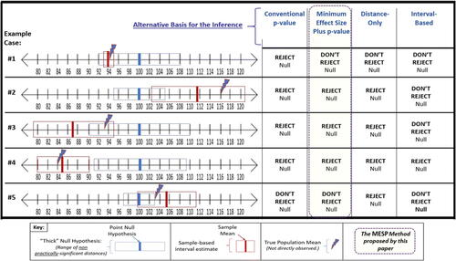
The real, but not directly observable, population mean for each example case is shown with a lightning bolt. The blue rectangle for each case (labeled “‘Thick’ Null Hypothesis” in the key) represents the range of values for the scenario that would be considered not meaningfully different from equaling the null mean, identified as the central blue line. Based on a case’s random sample drawn from the true population, the sample mean is shown as a vertical red line, with a surrounding red rectangle to signify a sample-based confidence interval for the estimate. Example Case #4 illustrates what is needed for all four methods to output the same inference indication that the evidence goes against the null: The p-value is low, and the sample mean and confidence interval around the sample mean lie beyond the thick null interval. #5 illustrates a scenario where the sample mean is beyond the thick null, which triggers a correct decision to Reject by Distance-only, yet the methods looking for a low enough p-value or for no overlap of thick null with the sample confidence interval estimate, do not reject in this instance. On the other hand, Example Case #1 shows a p-value-based decision to reject that is inconsistent with the mean’s true location (which is within the thick null).

3 Results

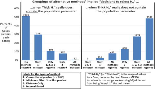
Figure 2 highlights a particular weakness of the p-value-based inference method compared to some alternatives, when the inference decision is to reject a null hypothesis that the population mean equals a specific value. If the true parameter is not meaningfully different from the null value (i.e., if the thick null is true), then a decision to reject the null would be in error. The left panel of Figure 2 shows that when the thick null was really true, the p-value-based method erred by rejecting it in 40% of the cases—often on its own (second bar) and sometimes it erred along with other methods (3rd and 5th bars). The alternative methods all performed better in this regard. The right panel shows that the p-value-based inferences were much more successful when the thick null was actually false: Alone, or with other methods, the conventional p-value’s call to reject the null was correct in about 80% of the cases (represented in the 7th, 10th, and 11th bars).

Fig. 2 Inference-success rates for four alternative methods.

These reported percentages were moderately sensitive to sample size, but much more influential was how large was the thick null range for the inference (determined by the Minimum Practically Significant Distance) relative to the variability in the underlying population. These sensitivities were explored further in Tables 1–3.

Table 1 Impacts of power and method on overall inference success rates.

		Proportions of implied inferences that were consistent with the true location of the mean, for each combination of approach and power
Power ^a	Number of simulated cases	Conventional^b	Small alpha^c	MESP^d	Distance-only^e	Interval-based^f
$\ge 0.80$	4214	63.2%	71.1%	91.2%	91.2%	84.3%
0.30 to 0.80	2791	81.5%	78.9%	83.2%	83.2%	69.5%
< 0.30	2995	67.6%	54.0%	67.6%	78.5%	57.8%
Numbers of cases	10,000	6963	6817	8192	8518	7220

a Nominal power, as calculated for a z-test for the mean, given these inputs: $\mathit{\alpha }=0.05$; minimum detectable difference $=$ MPSD for the case; n = the simulated case’s sample size; and σ = the true population sigma for the case

b Two-tailed, p-value based test, $\mathit{\alpha }=0.05$

c Two-tailed, p-value based test, $\mathit{\alpha }=0.005$

d Minimum effect size plus p-value approach proposed in this article.

e Directly compares effect size to MPSD

f Compares the thick null interval with a sample-based confidence interval for the mean

Table 2 Impact of power, method, and true location of the null on inference success.

Does the true location fall within the bounds of the “thick null”?	Power ^a	Number of simulated cases	Proportions of implied inferences that were consistent with the true location of the mean, for each combination of approach, power, and true location of the mean
			Conventional^b	Small Alpha^c	MESP^d	Distance-Only^e	Interval-based^f
Yes (4652 Cases)	$\ge 0.80$	2436	37.1%	52.7%	90.4%	90.4%	99.7%
	0.30 to 0.80	1325	76.7%	92.9%	82.9%	78.9%	99.5%
	< 0.30	891	92.0%	98.9%	92.0%	56.9%	98.0%
No (5348 Cases)	$\ge 0.80$	1778	98.9%	96.5%	92.4%	92.4%	63.1%
	0.30 to 0.80	1466	85.8%	66.3%	83.4%	87.2%	42.4%
	< 0.30	2104	57.3%	34.9%	57.3%	87.6%	40.7%
Numbers of cases:		10,000	6963	6817	8192	8518	7220

a Nominal power, as calculated for a z-test for the mean, given these inputs: $\mathit{\alpha }=0,05$; minimum detectable difference $=$ MPSD for the case; n = the simulated case’s sample size; and $\mathit{\sigma }$ = the true population sigma for the case

b Two-tailed, p-value based test, $\mathit{\alpha }=0.05$

c Two-tailed, p-value based test, $\mathit{\alpha }=0.005$

d Minimum effect size plus p-value approach, proposed in this article.

e Directly compares effect size to MPSD

f Compares the thick null interval with a sample-based confidence interval for the mean

Table 3 Impact of relative MPSD and method on inference success.

Does the true location fall within the bounds of the “thick null”?	Decile for MPSD in population standard deviations^a	Number of simulated cases	Proportions of implied inferences that were consistent with the true location of the mean, for each combination of approach, relative MPSD, and true location of the mean
			Conventional^b	Small Alpha^c	MESP^d	Distance-Only^e	Interva-Based^f
Yes (4652 Cases)	1	184	91.8%	99.5%	91.8%	43.5%	96.2%
	2	259	90.0%	98.5%	90.0%	52.1%	99,2%
	3	359	85.0%	97.2%	85.2%	64.1%	99.4%
	4	429	82.8%	935%	86.2%	79.5%	99.1%
	5	532	75.9%	90.8%	85.2%	78.2%	99.2%
	6	524	66.0%	84.9%	84.9%	81.9%	99.4%
	7	580	56.6%	76.7%	86.2%	83.8%	99.3%
	8	579	49.9%	66.8%	88.1%	87.0%	99.5%
	9	596	35.2%	50.2%	93.0%	92.6%	99.8%
	10	610	16.6%	24.3%	95.2%	95.2%	99.7%
No (5348 Cases)	1	807	54.9%	34.3%	54.9%	91.6%	45.4%
	2	682	66.7%	43.3%	66.7%	90.3%	45.2%
	3	703	71.0%	50.6%	71.0%	85.8%	44.0%
	4	566	78.8%	61.3%	77.0%	86.2%	39.6%
	5	476	82.1%	64.3%	77.5%	85.1%	36.6%
	6	467	86.9%	74.9%	79.7%	83.9%	43.7%
	7	427	90.6%	79.6%	83.8%	88.1%	41.9%
	8	419	96.4%	90.9%	91.4%	92.1%	58.2%
	9	410	97.8%	93.7%	93.2%	93.9%	70.0%
	10	391	100.0%	98.7%	95.7%	95.7%	78.0%
Numbers of cases		10,000	6963	6817	8192	8518	7220

a These ranges of values for MPSD/$\mathit{\sigma }$ correspond to the deciles:

1: 0.000–0.1076: 0.349–0.421

2: 0.107–0.1677: 0.421–0.531

3: 0.167–0.2328: 0.531–0.750

4: 0.232–0.2909: 0.750–1.214

5: 0.290–0.34910: 1.214–5.000

b Two-tailed, p-value based test, $\mathit{\alpha }=0.05$

c Two-tailed, p-value based test, $\mathit{\alpha }=0.005$

d Minimum effect size plus p-value approach, proposed in this article

e Directly compares effect size to MPSD

f Compares the thick null interval with a sample-based confidence interval for the mean

Table 1 compares the overall success rates of the alternative methods, controlled for the nominal power of the cases’ inference conditions. Nominal power values were determined for each case in the simulation, based on conventional power calculations for a one-sample z-test for the mean, given: α = 0.05, σ equal the case’s true population standard deviation, n = the case’s sample size, and minimum detectable difference equal to the case’s MPSD. These power values are nominal, since even the p-value-based approaches were not z-tests (since researchers would not know the true σ), and the z-test power calculations do not apply directly to the other methods. Nonetheless, the power-based distinctions in the table reflect differences in sample sizes and relative MPSD and variance sizes, etc., that would be relevant in general for making successful inferences.

A fifth method, proposed by some to address the false discovery problem for novel discoveries, is included in the above comparison; this bases its results on a smaller-alpha version of a conventional t-test ($\alpha =0.005$). (See Appendix A2 for more discussion on false discovery rates (FDRs).) Success rates based just on method can be calculated from Table 1 by dividing each method’s case count by the total number of cases: 10,000. Distance-Only appears to perform the best by all these measures, followed by MESP. The authors caution, however, that depending on one’s research goals and context, a researcher may be more concerned with the risks of (true) Type I error or of (true) Type II error. Table 1 masks those distinctions by averaging the two error risks into a single number.

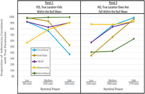
Table 2 breaks down the results of Table 1, based on whether the true mean falls within the thick null or falls beyond the thick null. Figure 3 displays this information graphically.

Fig. 3 Graph of impact of power, method, and true location of the null on inference success.

In the following discussions, power refers to nominal power unless true power is specifically indicated. A method’s true power is the proportion of really false thick nulls that the method correctly signals to Reject.

The various methods’ true powers are revealed by the success rates in the bottom half of Table 2. In all these cases, rejecting the null is the correct inference, since the real mean’s location is outside the thick null range. The conventional test stands up well against the alternatives in its true power to detect a difference from the null when there is a difference. For high nominal-power cases, it correctly rejected the false null almost 99% of the time and was correct 86% of the time for mid-power cases. When the null should be rejected in low-power cases, the conventional test does falter, as expected; in that scenario, only 57% of its inferences are correct. Interestingly, however, in low power cases, the only method that out-performs the conventional, α = 0.05 test is the distance-only approach, with a success rate of 88%.

Replacing the $P<$ 0.05 criterion with $P<$ 0.005 (small-alpha method) shows a considerable cost in true power for lower nominal-power cases. For the lowest-power cases, it only detects 35% of cases where there is really a meaningful difference from the null. However, when interpreting the small-alpha findings, a caution is that Benjamin et al.’s (2017) proposal for $P<$ 0.005 is specifically addressed to “novel discoveries,” that is, tests for rejecting the null where there is low prior probability for the alternative hypothesis being true. The simulation does not explicitly manipulate or control for that prior probability, when applying methods for comparison; so, the small-alpha results may not model an implementation of Benjamin et al.’s specific proposal with complete fidelity.

In trying to reduce Type I error (discussed next paragraph), the interval-based method pays a considerable price in true power: We see that for all levels of nominal power under the simulated conditions, the interval-based method has the worst or second-worst inference success when the null is really false. It outperforms only the small-alpha method when nominal power is low, with inference success of 41% in those cases compared to small-alpha’s 35%. The proposed MESP approach also has its main advantages regarding Type I error rather than for true power; yet we see that its benefits have little cost in terms of true power compared to the conventional test. For all nominal powers, MESP’s true power is comparable to the conventional approaches.

The top half of Table 2 shows methods’ rates of inference success (i.e., decisions to correctly not reject the null) when the real parameter is not meaningfully different from the null value (i.e., the thick null is true). A true Type I error occurs when the thick null is true yet is rejected (or a non-meaningful effect size is deemed meaningful, etc.); so, a method’s true Type I error rate (or true α) is the complement of its inference success rate for this half of the table. The table confirms the well-known limitation of conventional p-value tests when sample size (hence power) are large: For high-power cases where the thick null is really true, the conventional method’s true Type I error rate is a sobering 63% (based on 1— (successful inference rate = 37%)); for mid-power cases, its true α is 1 – 77% = 23%. The “α” in the conventional method’s “α = 0.05” criterion is clearly nominal; we see that the true α—the empirical Type I error rate for the method—is much higher. The small alpha approach predictably improves true Type I error rates, though they are still very poor for high-power cases, where the true α is 1 – 53% = 47%. The distance-only method, on the other hand, performs best under the simulated conditions for higher power cases: Its true α ranges from 1 – 90% = 10% for high-power cases to 1 – 57% = 43% for low-power cases.

The interval-based method implemented for this study outperforms all the displayed alternatives, with respect to true Type I error: never higher than 1 – 98% = 2%. But as mentioned with respect to the bottom half of the table, the method pays a considerable price in terms of true power.

MESP appears to offer a good compromise: Its true α stays comparatively low for all nominal power levels (ranging from 8% to 17%), while we observed its true power remains roughly comparable to conventional tests.

MESP’s combined use of a p-value and a distance criterion results in a notable pattern in Table 2: For both true and false thick nulls, MESP and distance-only methods perform identically when power is high, while the MESP and conventional methods perform identically when power is low. The reason is, when nominal power is high, MESP’s indication to reject or not-reject essentially hinges on the distance criterion’s signal (since getting a low p-value will be relatively easy to attain, and not the deciding issue). So, when the distance criterion leads to error in such cases (either rejecting a true null or not-rejecting a false one), the MESP shares in the error. But when nominal power is low, effect sizes tend to need to be larger to trigger the p-value reject signal (so attaining minimal distance is not the deciding issue); instead, MESP’s indication to reject or not reject tends to hinge on the p-value signal—so those methods share the same success and error rates.

A deeper analysis of the power breakdown in Table 2, with more power categories, is provided in Appendix A2, in Table A1.

All methods’ success rates are sensitive to relative MPSD, that is, the magnitude of the minimum practically significant distance (MPSD), relative to population standard deviation. These sizes ranged from (< 0.04 x σ) up to (5 x σ), and Table 3 breaks this size range into deciles. The discussion below focuses on Deciles 2 to 9 within each column. (Potential reliability issues of the outer deciles are discussed in Section 4.2 and Appendix A1).

In the top entries of the fourth column of Table 3, we see that the true Type I error rate (true α) for the conventional method is not a large concern when relative MPSD magnitudes are in the lowest deciles. In decile 2, true α was only about 10% (i.e., 1—90% successful inference rate for when thick null is true). But as relative MPSD increases, the conventional method’s true error rate increases consistently in tandem—reaching (1—35% successful = 65%) by the ninth decile. This occurs because the conventional method does not consider practical importance; a larger relative MPSD results in more cases where a value is rejected based on the null mean alone, yet is getting included in the expanded thick null, so it is an error to reject the null.

The conventional method’s true power to correctly reject a false null (bottom half of fourth column), increases consistently as relative MPSD increases. This is because, for subsets of the false-null cases which have wider thick null intervals, the p-value approach is assessing effect sizes that tend to be larger, and so is more likely to correctly reject the null for those cases.

The small-alpha approach’s success rates (fifth column) show similar directions of sensitivity to relative MPSD as for the conventional approach, across all deciles, for the same reasons as explained in the previous two paragraphs. The interval-based method that was modeled appears insensitive to relative MPSD size and is almost always correct when the thick null is true (top half of right column). Its generally poor true power to reject a false null improves a bit (about 70%) when MPSD is relatively large compared to σ (perhaps because this method is also sensitive to having a small σ, for reasons not related to MPSD.) The distance-only method appears comparatively insensitive to relative MPSD size for true power (bottom half of the seventh column). However, for small relative MPSD’s (top of the seventh column), the method’s true α rate is very poor: In the second decile, (1 – (52% success rate when the null is true) = 48%. This occurs because small differences that the method deems meaningful are often due simply to sampling error, which this method does not account for.

The MESP method generally maintains strong relative performance regardless of the size of MPSD/σ. The method’s true power is comparable, for all relative MPSD levels, with the conventional method’s; while it is true α rates (top half of the sixth column) never exceed 15% (in the sixth row, based on 1—85% success).

Table A2 in the appendix shows how the effects of power and relative MPSD size combine. For example, the lowest inference success rate (37%) displayed in Table 2 is for the conventional test, when nominal power is high and the thick null is true. If that context is subdivided based on relative MPSD size, then consistently with Table 3, the lower success rates are more specifically occurring as relative MPSD increases: 62% success for the second quartile but down to 49% for the third quartile, etc. Because some of the simulated combinations of power and relative MPSD in Table A2 would, if they occurred in practice, reflect conditions of poor study design or execution, such cases may be overrepresented in the simulation, which could affect the reported findings.

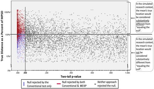
Figure 4 illustrates how p-values combined with a distance criterion can be informative for inference as heuristic cues, as discussed in Section 1.2—even though p-values on their own are noisy as predictors of whether a thick null is really false or true. The figure plots, for each case in the simulation, the true distance of the parameter from the null (Y-axis), versus the two-tailed p-value that was generated for that case (X-axis). For any case shown below the central horizontal line, the distance of the true parameter value from 100 is less than the minimum practically significant distance, consistent with the thick null being correct; above the line the thick null would not be correct. (Logarithmic scales for the axes are simply to make the graph’s salient features more visually prominent, with less blank space.) Cases where the MESP inference procedure would signal to reject the null are displayed as the red, horizontal lines; this rejection signal is seen to clearly, though imperfectly, be associated with cases when the thick null really is false. In other words, obtaining the MESP signal-to-reject provides a heuristic, yet nondefinitive, piece of evidence toward inferring the mean’s true location.

Fig. 4 p-Value’s inference performance, compared to MESP.

4 Model Assumptions and Limitations

4.1 Representativeness of the Model

Although the authors believe that the versions of methods included in the simulation model are reasonably generic and representative of the methods discussed, the generality of the model has not been formally tested or demonstrated for nonincluded variations. The applicability of the results for one-tailed tests was checked in Appendix A2, Table A4, and the simulation results there appear comparable to those in Table 2 for two-tailed tests.

Results reported for the interval-based method may not fully extend to a recent variation of the method proposed by Blume et al. (2018). Both versions signal to reject the null when the thick null interval and a sample-based 95% confidence interval (CI) do not overlap. But absent that signal, Blume et al. distinguish (a) when the null interval subsumes the CI completely versus (b) when the intervals’ overlap is only partial. The impact if any of that added distinction is not modeled in the present study.

4.2 Generation of Data for Cases

The design choices made in this study for generating set-up values from particular input-ranges can impact the comparative decision results that are reported. This echoes the insight of Bayesians that prior probabilities can impact posterior probabilities. It is not possible to make absolute inferences based on observed data, without some reference to the context in which the data are drawn. For example, combinations of set-up values generated by the simulation were not assigned different weights for being more or less likely to be encountered, though in some research contexts, perhaps some combinations are more or less likely. Therefore, the exact numbers reported in the Results section for true power and true α, etc., cannot be interpreted in absolute terms. In general, more research is needed on the extent and nature of the simulation’s sensitivity to unmodeled differences in actual likelihoods, for different combinations of scenarios or extremes of distributions generated by the simulation.

More detailed discussions on the design decisions for the generated set-up values and their impacts on the overall distributions of the test cases, and on the plausibility of those distributions to represent a realistic example set, are provided in Appendix A1.

4.3 Risks of MPSD “Hacking”

An acknowledged risk of including a distance criterion within MESP is that researchers could potentially “hack” results by setting MPSD sizes that are biased or specified-post hoc to their own study’s advantage. The authors believe this issue is important, but that it should be viewed as primarily a matter of professional ethics and training, and also that risks for such tainting are not inherently different for MESP than those for any inference method—for example, one’s selecting a more favorable α or Cohen’s d benchmark post hoc. The authors recommended in Section 1.1 that MPSD values should derive from a researcher’s reflective professional practice, and be documented along with his or her results. This suggestion is consistent with proposals that research benchmarks of this sort be preregistered in some way before starting one’s study. The authors also encourage efforts for the research community at large to become more sensitive to issues of effect size. For example, if the data include strong measures such as amounts of money spent or cigarettes smoked over a period of time, unstandardized regression weights can inform whether the impact of a one unit increase in the independent variable really has an appreciable impact on the dependent variable; such as, is the impact just a small number of extra or fewer dollars spent or cigarettes smoked over the period, or is the increase or reduction in dozens or hundreds of dollars or cigarettes?

Note that in the simulation, random assignments of MPSDs to cases is not intended to imply that MPSDs’ assignments to actual research would or should be random—just as sample sizes would not be random in practice but are assigned randomly in the simulation. The goal for the simulation was to generate many different combinations of independently generated set-up values, to observe the factors’ effects and interactions. Each simulated case is taken to represent data collected by a specific (simulated) researcher who would have set that study’s MPSD value competently and appropriately, in the context of his or her research specialty.

5 Discussion and Conclusions

This study confirms, using simulations, that p-values provide some evidential information relevant to an inference about a population mean, given a sample. It examines p-values’ strengths and weaknesses if used as an inference signal in various contexts, and compares these with successes and weaknesses of some alternative methods. Among these, an alternative, hybrid inference method is introduced, which uses a criterion called minimum effect size plus p-value (MESP).

Key findings from the simulation are summarized below:

• For tests that were high nominal powered (e.g., large samples; small population variance), the p-value-only approaches had the worst true Type I error rates. Specifically, for conventional $P<$ 0.05 tests with high nominal power, true α was 63%. For small alpha tests, true α was 47% with nominal high power. For both versions of p-value tests compared, true α increases markedly (i.e., inference success drops) as the thickness of the null increases.

• Both p-value methods have good true power when nominal power is high. But for small alpha true power drops to under 40% for low nominal power cases, or when the relative MPSD is small. Conventional ($P<$ 0.05) performs better in those circumstances.

• The distance-only method falters in true α ($\alpha =43\%$) for low-power cases, or when relative MPSD is comparatively small. The method has good true power (> 87%) for all nominal power levels and relative thicknesses of the null.

• A generic interval-based method has consistently good true α for all nominal power levels and relative thicknesses of the null—never worse than 2%. But for all nominal powers, its true power is much less than the conventional methods.

• MESP balances reasonably consistent true power (roughly equivalent with the ($P<$ 0.05) at all nominal powers and relative thicknesses of the null, with a true α that compares well with other methods—without other methods’ problems with some nominal power levels or thicknesses of the null.

• Changing from two- to one-tailed tests does not appreciably change the performance patterns described for the p-value and MESP approaches.

• A method that combines p-values with a distance criterion can generate heuristic, but nondefinitive, evidence toward inferring a mean’s location—even though p-values on their own are noisy as predictors of the mean’s true location.

The percentages reported could potentially be different under different—yet plausible—simulated conditions.

In summary, all of the compared methods have strengths and weaknesses; and none of them generates an automatic final answer for a definitive inference, based on one application. In practice, the researcher is blind to the left columns of Tables 2 and 3, which show the true mean, and this makes a crucial difference: The interval-based method is, for example, the best method under the simulated conditions when the null is true, but the worst method under those conditions when the null is false. But the researcher cannot know which half of that column he or she is really working in.

The authors recommend preferring a tool that (a) is not sensitive to factors that are not knowable to the researcher (such as the true mean, and to a lesser extent, the true size of MPSD relative to population sigma), and (b) performs well in contexts that the researcher can check for. MESP performs well regardless of whether the unseen real mean happens to be within the thick null or not. Its true power weakens in low nominal power cases; but the researcher can know when that applies, and can respond accordingly.

Added to those advantages for MESP is the ready availability of the p-value component of its indicator. Statistical software can already flag when a correlation or regression coefficient or other estimate appears significant, in terms of the $p<$ 0.05 signal. If a researcher also has in mind a reasoned criterion for a meaningful effect size, MESP can be directly applied to the case, without requiring any new type of calculations. In contrast, data to implement the procedures for the interval-based method may not be visible on standard outputs, and may require additional, unfamiliar calculations.

As noted in Section 4, the exact success ratios displayed in this article’s text and tables are specific to the design decisions for the simulations. Choosing a p-value criterion other than 0.05 or 0.005, or designing alternative algorithms for distance-only or interval-based decisions, or revising the bounds of possible inputs for the simulation, etc., could all impact apparent results. Yet, the versions of methods compared in this study, and the ranges of independently varied random set-up factors for cases, were designed to generate a dataset of cases that the authors believe are reasonably representative of real-research cases and methods that could be encountered. Informal, additional checks were also conducted (such as adapting the simulation to assess tests for correlation rather than for the mean); and the broad patterns of the results reported here appear to be generalizable.

The usefulness of any inference method’s results depends on the care taken to ensure that all fundamental assumptions are satisfied for using that method—not just assumptions specific to that method, such as distributional assumptions, but also, more generally, having an unbiased, representative sample, with no unacknowledged confounders influencing results, or missing variables causing proxy effects, and so on. The comparisons presented in this article are intended to the compare the findings of the several methods so far as they have been carefully and properly implemented, under circumstances that meet their assumptions.

With that proviso, the authors believe that the NHST model can still have a place in scientific research and in the journalistic reporting of research findings if results are interpreted properly and not taken as automatically justifying final conclusions. If the p-value criterion is met, it should also be assessed whether a meaningful minimum effect size was observed. MESP combines the traditional p-value < 0.05 condition with a minimum effect size criterion. The simulations show that even for the traditional method, “α = 0.05” is essentially just a nominal trigger, it is not the true α; MESP merely acknowledges this heuristic use of the α term and adds the important effect-size criterion. If the two rejection criteria for MESP occur, take that cue and build a convincing story using full disclosure on sampling methods, sample size and what is already known, unknown or hypothesized.

Appendix A.

Additional Analyses and Simulation Details

A.1 Distributions of Set-up Values and Their Combinations

How realistic or generalizable the simulation’s results are could be impacted by the distributions of the set-up values that were randomly generated over the 10,000 passes of the simulation—or of the relations among those values. This appendix displays and discusses several of those key distributions.

• Individual Set-up Values

For each pass of the simulation, set-up values for each of $\mathit{\mu }$, $\mathit{\sigma }$, n, and MPSD were independently determined by randomly selecting an integer from a specified range of equiprobable integer values for that element: Those ranges were 75 $\le$ $\mathit{\mu }$ $\le$ 125; 4 $\le$ $\mathit{\sigma }$ $\le$ 60; 5 $\le$ n $\le$ 100; and 2 $\le$ MPSD $\le$ 20. Figure A1 shows that—allowing for random variation—the distributions are all flat as intended by the study, and bounded within the designed ranges.

• Combinations of Set-up Values

Each pass of the simulation is intended to model a realistic example of a hypothesis test for a population mean that might be conducted, with respect to the actual values that $\mathit{\mu },\mathit{\sigma }$, n, and MPSD may have when the test is conducted. The limits bounding an example’s being realistic are difficult to define formally; but some potential issues can be intuited and addressed in connection with the following results.

Since H₀ is unvaried in the simulation, the relation between mean and sigma that is relevant for the simulated hypothesis tests is the ratio $|\mu -H_0|$/σ, that is, the absolute real distance of the population mean from the null mean, in standard deviations. Figure A2 shows that most of the simulated true distances had a magnitude of less than one population standard deviation, and very few magnitudes exceeded 2.5 standard deviations. Occasionally in practice, researchers may be unaware if they have posited a null value that far from the true μ (perhaps because an unobserved change occurred in the environment), so the few outliers like this generated in the distribution are not necessarily implausible, and are useful for comparing the different inference methods’ performance in such cases.

In most cases, the values for relative MPSD—that is, MPSD standardized relative to population standard deviation (MPSD/σ)—were very consistent with effect sizes that, for example, researchers would want to power their studies to detect. Assuming a researcher has obtained a reasonable, preliminary estimate for the population standard deviation σ, then it may be unrealistic that MPSD would be set deliberately to large values like two or more standard deviations. However, note that large MPSD/σ ratios of this sort in Figure A3 occur only within the uppermost decile of the distribution. Also, the lowest decile is of interest, since it roughly corresponds to a smaller setting of MPSD—0.1 standard deviation—that social scientists sometimes employ. Table 3 in the main text groups MPSD/σ values into deciles, in order to observe the comparative impacts of relative MPSD sizes at various levels, including the more extreme categories.

The potential distortion that large sample sizes can have on conventional test results is often discussed. However, the derivation on the right panel of Figure A4 clarifies, more specifically, that the test statistic is inflated (lowering the p-value) by the ratio of $\surd n$ to σ. Even though the simulation has capped the set-up values for n at 100, some cases’ results could be distorted if n is large and σ is small; however, according to the histogram in the figure’s left panel, this “multiplier” ratio for the test statistic does not appear to have an excessive spread for the simulated data. Larger values could realistically occur if a researcher has access to larger sample sizes, and takes advantage of them, while perhaps is not certain of the true sigma value when estimating sample size or power.

Figure A5 shows the distribution of ratios generated by the simulation for absolute real distances (i.e., $|\mu$ - $H_0|)$ over MPSD. For cases where the true mean falls within the thick null (top half of Tables 2 and 3), that ratio is $\le$ 1; where that ratio is > 1, the true mean falls beyond the thick null (bottom half of Tables 2 and 3).

The simulation did not exclude any cases based on this ratio, since it was not known, a priori, whether it would be realistic for ($|\mu$ - $H_0|)$/MPSD to have a ratio as large as, for example, 6 or greater. This suggests questions for further research: (a) How do actual researchers set the values they would use for MPSD? (b) In particular, do they include in their reasoning some estimate of how far from the null the true mean could realistically fall? (c) If so, how do they derive their belief or expectation about how far that could be, and (d) do they generally tend to be accurate in that estimate.

A.2 Additional Analyses of Methods’ Inference Success

• Impact of Power and Method on Inference Success (Expanded)

Table A1 deepens the analysis in Table 2, by breaking power into six categories instead of the three categories used in the main text. The finer-grain analysis in Table A1 preserves the general value trends displayed in Table 2 for each status of the thick null, when scanning down the alternative methods’ columns. However, for the highest or lowest power categories, sudden value jumps do occur in some columns. For example, when the thick null is true, the success rate of the conventional method decreases monotonically as power increases—yet the drop is 30 percentage points from second-highest to the highest power category. And that method’s success rate drops 20 percentage points at the lowest power category, when the thick null is incorrect. It would useful in future research to investigate for any factors, unmodeled in the simulation, that may contribute to these sudden jumps.

• Impact of Combined Power and Relative MPSD on Methods’ Inference Success Rates.

Tables A2 and A3 supplement the stand-alone analyses in the main text for the impacts of Power (Table 2) and relative MPSD (Table 3), respectively, on different methods’ inference success rates. Table A2 looks at the impact of the two factors combined. To reduce the complexity of the table, the sub-classes for MPSD/σ are based on quartiles rather than deciles for the distribution. Table A3 supports using that simplification of classes for relative MPSD: Namely, if values up and down individual columns in Table A3 (Quartile-based) are directly compared with counterparts in Table 3 (Decile-base), it is observed that dividing the data more finely into deciles uncovers no reversals or inconsistency of the general trends that can be observed using quartiles.

• Impact of Power on Methods’ Inference Success Rates—One-tailed Cases

Table A4 and Figure A6 suggest that the results would be very similar for one-tailed tests, as for two-tailed tests. Only the cases of the main simulation where μ > 100 are evaluated in this section, presuming contexts where the true mean could not realistically be less than that null; and one-tailed p-value calculations were applied where applicable. The small-alpha method was not evaluated for this table.

When comparing relative strengths and weaknesses of different methods, broken down by whether the thick null is true, and nominal power levels, Table A4 (for one-tailed cases) is clearly very similar to Table 2 (for two-tailed cases). Apart from small random variations (from reducing the set of relevant cases included), Table A4’s differences from Table 2 are as expected: For a given p-value cutoff, a one-tailed test does not require as large an effect size (in the one direction of interest) as a two-tailed test does to reject a null hypothesis. Therefore, at all nominal power levels, the one-tailed conventional test shows a bit more power to reject the null when the thick null is really false yet has poorer success rates (i.e., more true Type I error) when the thick nulls are really true. Because of its extra distance criterion, MESP did not display that same increase in true power, for one-tailed versus two-tailed decisions, for the cases with the highest nominal power. For one-tailed tests, for all but the lowest-powered cases, MESP continues to show better success when the thick null is true (smaller true $\alpha )$ compared to the conventional method.

• FDRs Comparisons and Implications

Sometimes, many tests are conducted simultaneously, for example, in multiple testing of biological materials on “microarrays.” Each of the many tests simulated for this study—even if they were simultaneous—models a stand-alone hypothesis test, with different set-up values. Still, this partial analogy with multiple-testing suggests a useful concept to consider, called FDR, which may also suggest a potential limitation of the simulation design.

In the microarrays analogy, each individual test that rejects the null (i.e., each “discovery”) could be interpreted as testing positive for a condition of interest. The FDR is a way to quantify, for comparisons and quality assessment, the overall rate of false positives across all the simultaneously conducted tests (Colquhoun 2014). FDR is calculated by dividing the number of false-positive test results (when there is really no effect) by the sum of all positive test results (the number of false positives + the number of true positives).

Figure A7 compares methods’ relative successes by FDR, where a lower value is preferable. There are rough similarities to the results in the upper half of Table 2 (not controlling for nominal power); but FDR factors in information from both halves of Table 2—both real effect cases and no effect cases.

To calculate FDR in practice, the process (depicted in Colquhoun’s “Figure 2” (2014, p. 4)) requires the ratio of real effects cases to no effects cases to first be estimated in advance; and, from this prior estimate, expected counts of true and false positives to be estimated in turn. In Figure A7, the counts in the boxes are not estimated, but are observed directly from the simulation results. Yet, that said, the counts and ratios of inference successes displayed in Figure A7 do depend on the prior ratio of real to no effects generated by the simulation (in the second column of boxes); and that ratio could have been quite different—if for example, the simulated true means were all far from the null, so real effects were more prevalent. This reflection echoes the observation made with respect to Figure A5, for the simulation’s distribution of (absolute real distance)/MPSD. Further study of what distributions and scenarios would be most realistic to embody in the simulation is recommended.

Supplementary Material

1. Title: Comparative Inference Experiments_Data and Formulas (Excel file)

Simulation results and formulas. This Excel file contains the full set of outputs (10,000 cases) for the simulation run described in the article. It also includes pages showing (a) all formulas used within the simulation, and (b) explanations of the formulas.

Note that for the output columns generated during the simulation run, only the resulting numeric values of the outputs are included in the Results spreadsheet; whereas for supplemental columns added to the Results spreadsheet—for example, to calculate nominal power for each case or to calculate what would have been the one-tailed p-value for each case—the formulas are retained in the spreadsheet in those extra columns.

2. Title: Supplemental_Key Algorithms Implemented (PDF file)

Generic descriptions of algorithms. This PDF document provides brief, generic descriptions of key algorithms and formulas implemented in this article’s simulation.

Fig. A1 Distributions of the individual set-up values.

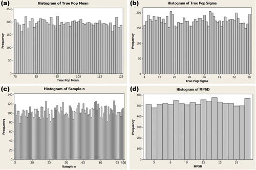
Fig. A2 Histogram of absolute real distances in population standard deviations.

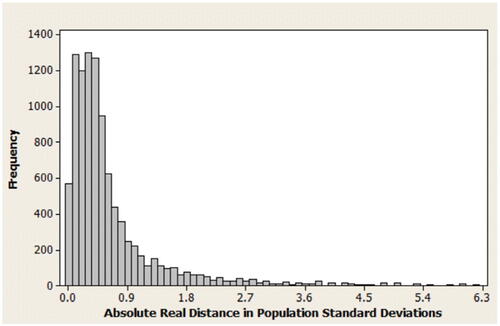
Fig. A3 Absolute and cumulative percent frequencies for MPSD/σ.

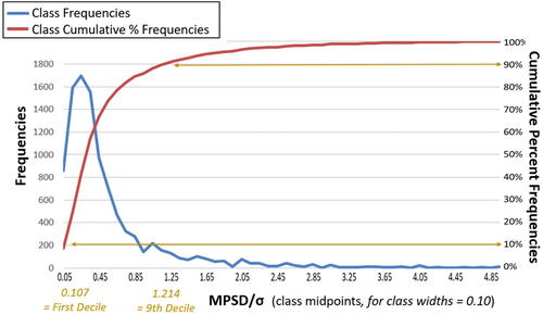
Fig. A4 Ratio of $\surd$n to $\mathit{\sigma }$.

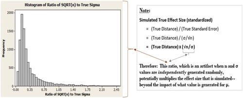
Fig. A5 Ratio of absolute real distance to MPSD.

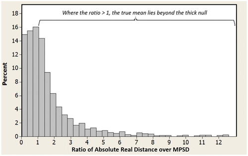
Fig. A6 Graph of Impact of power and method on inference success, for one-tailed cases.

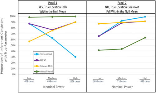
Fig. A7 Methods’ False-positive rates compared.

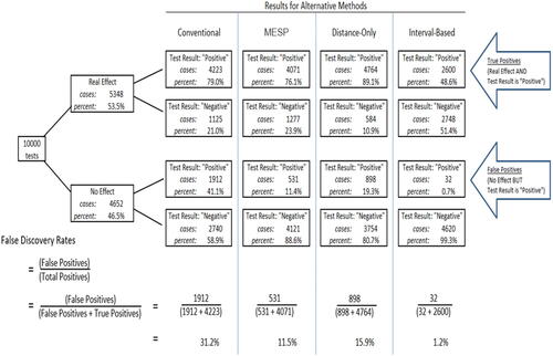
Table A1 Impact of power and method on inference success rates—expanded version.

Does the true location fall within the bounds of the “thick null”?	Nominal power	Number of simulated cases	Proportions of implied inferences that were consistent with the true location of the mean, for each combination of approach, power, and true location of the mean
			Conventional	Small alpha	MESP	Distance-only	Interval-based
Yes	$\ge 0.90$	2075	32.8%	47.1%	91.3%	91.3%	99.7%
	0.80–0.90	361	62.0%	84.8%	85.0%	85.0%	100.0%
	0.60–0.80	542	68.8%	88.4%	81.7%	81.5%	99.3%
	0.40–0.60	489	81.8%	95.7%	84.3%	80.4%	99.6%
	0.20–0.40	575	85.7%	97.2%	85.9%	71.0%	99.1%
	< 0.20	610	93.4%	99.3%	93.4%	50.7%	97.7%
No	$\ge 0.90$	1475	99.7%	98.8%	93.5%	93.5%	66.0%
	0.80–0.90	303	95.4%	85,1%	87.1%	87.1%	48.8%
	0.60–0.80	502	92.4%	76.7%	86.9%	87.3%	43.0%
	0.40–0.60	590	87.1%	65.1%	85.8%	88.6%	41.4%
	0.20– 0.40	840	73.1%	50.8%	73.1%	86.0%	43.9%
	< 0.20	1638	53.2%	31.2%	53.2%	87.8%	39.6%
Numbers of cases		10,000	6963	6817	8192	8518	7220

Table A2 Impact of combined power and relative MPSD on methods’ inference success rates.

Does the true location fall within the bounds of the “thick null”?	Power^a	Quartile for MPSD in population standard deviations^b	Number of simulated cases	Proportions of implied inferences that were consistent with the true location of the mean, for each combination of approach, relative MPSD, nominal power, and true location of the mean.
				Conventional^c	Small alpha^d	MESP^e	Distance-only^f	+--
	$\ge 0.80$	1	–	–	–	–	–	–
		2	126	61.9%	81.7%	81.0%	81.0%	100.0%
		3	879	49.0%	69.6%	86.5%	86.5%	99.7%
		4	1431	27.6%	39.7%	93.6%	93.6%	99.7%
	0.30–0.8	1	87	79.3%	94.3%	79.3%	69.0%	100.0%
Yes		2	745	77.4%	92.S%	83.2%	79.9%	99.7%
(4652 Cases)		3	423	74.7%	92.4%	83.0%	73.7%	99.1%
		4	70	77.1%	95.7%	84,3%	81.4%	98.6%
	< 0.30	1	518	91.5%	99.0%	91.5%	50.4%	98.1%
		2	297	92.9%	98.3%	92.9%	65.3%	97.6%
		3	74	91.9%	100.0%	91.9%	67.6%	98.6%
		4	2	100.0%	100.0%	100.0%	100.0%	100.0%
	$\ge 0.80$	1	–	–	–	–	–	–
		2	113	96.5%	85.8%	84.1%	84.1%	48.7%
		3	701	98.3%	95.7%	90.2%	90.2%	51.5%
		4	964	99.7%	98.2%	95.0%	95.0%	73.2%
	0.30–0.80	1	185	82.2%	60.5%	82.2%	87.6%	51.9%
No		2	908	881%	71.7%	85.8%	88.3%	42.8%
(5348 Cases)		3	324	83.0%	59.3%	78.7%	84.6 %	36.4%
		4	49	75.5%	34.7%	73.5%	81.6 %	36.7%
	< 0.30	1	1656	60.3%	37.9%	60.3%	90.9%	44.3%
		2	378	47.9%	25.9%	47.9%	76.7%	28.8%
		3	69	37.7%	13.0%	37.7%	68.1%	20.3%
		4	1	100.0%	0.0%	100.0%	100.0%	0.0%
Numbers of cases			10,000	6963	6817	8192	8518	7220

a Nominal power, as calculated for a z-test for the mean, given these inputs: $\mathit{\alpha }$ = 0.05; minimum detectable difference_MPSD for the case; n = the simulated case’s sample size; and $\mathit{\sigma }$= the true population sigma for the case.

b These ranges of values for MPSD/$\mathit{\sigma }$ correspond to the Quartiles: 1: 0.000 to 0.200 2: 0.200 to 0.349 3: 0.349 to 0.615 4: 0.615 to 5.000

c Two-tailed. p-value based test, $\mathit{\alpha }$ = 0.05

d Two-tailed, p-value based test, $\mathit{\alpha }$ = 0.005

e Minimum effect size plus p-value approach, proposed in this article.

f Directly compares effect size to MPSD.

g Compares the Thick Null Interval with a sample-based confidence interval for the mean.

Table A3 Impact of relative MPSD on methods’ inference success rates—using quartiles.

Does the true location fall within the bounds of the “thick null”?	Quartile for MPSD in population standard deviations^a	Number of simulated cases	Proportions of implied inferences that were consistent with the true location of the mean, for each combination of approach, relative MPSD, and true location of the mean
			Conventional^b	Small alpha^c	MESP^d	Distance-only^e	Interval-based^f
Yes	1	605	89.8%	98.3%	89.8%	53.1%	98.3%
	2	1168	79.7%	93.0%	85.4%	76.3%	99.2%
	3	1376	59.2%	78.3%	85.7%	83.1%	99.4%
	4	1503	30.0%	42.4%	93.2%	93.1%	99.7%
NO	1	1841	62.5%	40.2%	62.5%	90.5%	45.1%
	2	1399	77.9%	60.5%	75.4%	84.8%	39.5%
	3	1094	89.9%	79.7%	83.5%	87.1%	45.1%
	4	1014	98.5%	95.1%	94.0%	94.4%	71.4%
Numbers of cases:		10,000	6963	6817	8192	8518	7220

a “1”: <0.200 “2”: 0.200 to 0.349, “3”: 0.349 to 0.615, and “4”: 0.615 to 5.000

b Two-tailed, p-value based test, α = 0.05.

c Two-tailed, p-value based test, α = 0.005.

d Minimum effect size plus p-value approach, proposed in this article.

e Directly compare effect size to MPSD.

f Compares the thick null interval with a sample-based confidence interval for the mean.

Table A4 Impact of power and method on inference success, for one-tailed cases.

Does the true location fall within the bounds of the “thick null”?	Power^a	Number of simulated cases	Proportions of implied inferences that were consistent with the true location of the mean, for each combination of approach, power, and true location of the mean.
			Conventional^b	MESP^c	Distance-only^d	Interval-based^e
Yes (2217 Cases)	$\ge 0.80$	1156	30.3%	90.2%	90.2%	99.7%
	0.30 to 0.80	653	62.6%	76.9%	75.5%	99.2%
	< 0.30	408	87.5%	87.5%	56.9%	98.5%
No (2636 Cases)	$\ge 0.80$	896	99.2%	91.4%	91.4%	63.2%
	0.30–0.80	710	92.4%	88.7%	89.4%	43.5%
	< 0.30	1030	65.8%	65.8%	87.2%	41.7%
Numbers of cases		4853	3339	4029	4120	3507

a Nominal power, as calculated for a z-test for the mean, given these inputs: $\mathit{\alpha }$ = 0.05; minimum detectable difference = MPSD for the case; n = the simulated case’s sample size; and $\mathit{\sigma }$ = the true population sigma for the case

b One-tailed, p-value based test α = 0.05.

c Minimum effect size plus p-value approach, using the p-value for one-tailed.

d Directly compares effect size to MPSD.

e Compares the thick null interval with a sample-based confidence interval for the mean.

References

- Benjamin, D.J., Berger, J., Johannesson, M., Nosek, B. A., Wagenmakers, E.-J., Berk, R., …, Johnson, V. (2017, July 22). “Redefine Statistical Significance,” PsyArXiv Preprints (Online), available at https://psyarxiv.com/mky9j
- Berger, J.O., and Delampady, M. (1987), “Testing Precise Hypotheses,” Statistical Science, 2(3), 317–352. DOI: 10.1214/ss/1177013238.
- Berger, J.O., and Sellke, T. (1987), “Rejoinder to Comments on ‘Testing a Point Null Hypothesis: The Irreconcilability of p Values and Evidence,”’ Journal of the American Statistical Association, 82(397), 135–139. DOI: 10.2307/2289139.
- Blume J.D., D’Agostino McGowan, L., Dupont W.D., Greevy, R.A. Jr (2018) “Second-Generation pValues: Improved Rigor, Reproducibility, & Transparency in Statistical Analyses,” PLoS ONE, 13(3): e0188299, available at DOI: 10.1371/journal.pone.0188299.
- Chow, S.L. (1988), “Significance Test or Effect size?” Psychological Bulletin, 103, 105–110. DOI: 10.1037/0033-2909.103.1.105.
- Cohen, J. (1988), Statistical Power Analysis for the Behavioral Sciences (2nd ed.), Hillsdale, NJ: Lawrence Erlbaum Associates.
- Colquhoun, D. (2014), “An Investigation of the False Discovery Rate and the Misinterpretation of p-values,” Royal Society Open Science, 1: 140216. DOI: 10.1098/rsos.140216.
- Ellis, P.D. (2010), The Essential Guide to Effect Sizes: Statistical Power, Meta-Analysis, and the Interpretation of Research Results, Cambridge, UK: Cambridge University Press.
- Fisher, R. A. (1925), Statistical Methods for Research Workers (1st ed.), Edinburgh, Scotland: Oliver & Boyd. [Chapter 3, 5th paragraph.]
- Folger, R. (1989), “Significance Tests and the Duplicity of Binary Decisions,” Psychological Bulletin, 106, 155–160. DOI: 10.1037/0033-2909.106.1.155.
- Goodman, W.M. (2010), “The Undetectable Difference: An Experimental Look at the ‘Problem’ of p-Values,” in American Statistical Association JSM Proceedings, available at http://www.statlit.org/pdf/2010GoodmanASA.pdf.
- Greenland, S. (2017). “Invited Commentary: The need for Cognitive Science in Methodology,” American Journal of Epidemiology, 186, 639–645. DOI: 10.1093/aje/kwx259.
- Howard, G.S., Maxwell, S.E., and Fleming, K.J. (2000), “The Proof of the Pudding: An Illustration of the Relative Strengths of Null Hypothesis, Meta-Analysis, and Bayesian Analysis,” Psychological Methods, 5(3), 315–332. DOI: 10.1037/1082-989X.5.3.315.
- Krueger, J.I., and Heck, P. R. (2017), “The Heuristic Value of p in Inductive Statistical Inference,” Frontiers in Psychology, available at http://journal.frontiersin.org/article/10.3389/fpsyg.2017.00908/abstract
- Lakens, D., Adolfi, F. G., Albers, C. J., Anvari, F., Apps, M. A. J., Argamon, S. E., …, Zwaan, R.A. (2018). “Justify your Alpha,” Nature Human Behavior, 2, 168–171. DOI: 10.1038/s41562-018-0311-x.
- Leek, J.T. and Peng, R.D. (2015), “Statistics: p-Values are Just the Tip pf the Iceberg,” Nature, 520, 612, available at https://www.nature.com/polopoly_fs/1.17412!/menu/main/topColumns/topLeftColumn/pdf/520612a.pdf
- Meehl, P.E. (1967), “Theory Testing in Psychology and in Physics: A Methodological Paradox,” Philosophy of Science, 34, 103–115. DOI: 10.1086/288135.
- Nunnally, J. (1960), “The Place of Statistics in Psychology,” Educational and Psychological Measurement, 20, 641–650. DOI: 10.1177/001316446002000401.
- Nuzzo, R. (2015), “Scientists Perturbed by Loss of Stat Tool to Sift Research Fudge from Fact,” Scientific American [online], available at https://www.scientificamerican.com/article/scientists-perturbed-by-loss-of-stat-toolstosift-research-fudge-from-fact/.
- Peng, R. (2015), “The Reproducibility Crisis in Science: A Statistical Counterattack,” Significance, 12(3), 30–32. DOI: 10.1111/j.1740-9713.2015.00827.x.
- Siegfried, T. (2015), “P Value Ban: Small Step for a Journal, Giant Leap for Science,” Science News [online], available at https://www.sciencenews.org/blog/context/p-value-ban-small-step-journal-giant-leapscience.
- Trafimow, D, Amrhein, V, Areshenkoff, C.N., Barrera-Causil, C.J., Beh, E.J., Bilgiç, Y.K., …, Marmolejo-Ramos, F. (2018) “Manipulating the Alpha Level Cannot Cure Significance Testing,” Frontiers in Psychology, 9, 699, available at https://www.frontiersin.org/articles/10.3389/fpsyg.2018.00699/full
- Trafimow, D. and Marks, M. (2015), Editorial, Basic and Applied Social Psychology, 37(1), 1–2. DOI: 10.1080/01973533.2015.1012991.
- Wasserstein, R.L., and Lazar, N.A. (2016a), “The ASA’s Statement on p-Values: Context, Process, and Purpose (Editorial, March 7, 2016),” The American Statistician, 70(2), 129–133.
- Wasserstein, R.L., and Lazar, N.A. (2016b), “The ASA’s Statement on p-Values: Context, Process, and Purpose. Figshare, The American Statistician [online, supplemental materials] (March 7, 2016), available at https://figshare.com/collections/The_ASA’s_statement_on_p_values_context_process_and_purpose/2851090/1.
- Wetzels, R., Matzke, D., Lee, M.D., Rouder, J.N., Iverson G.J., and Wagenmakers, E.J. (2011), “Statistical Evidence in Experimental Psychology: An Empirical Comparison Using 855 t Tests,” Perspectives on Psychological Science, 6(3), 291–298. DOI: 10.1177/1745691611406923.
- Woolston, C. (2015), “Psychology Journal Bans p-Values,” Nature, 519, 9, available at http://www.nature.com/news/psychologyjournalbans-p-values-1.17001.