Multiple Perspectives on Inference for Two Simple Statistical Scenarios

ABSTRACT

When data analysts operate within different statistical frameworks (e.g., frequentist versus Bayesian, emphasis on estimation versus emphasis on testing), how does this impact the qualitative conclusions that are drawn for real data? To study this question empirically we selected from the literature two simple scenarios—involving a comparison of two proportions and a Pearson correlation—and asked four teams of statisticians to provide a concise analysis and a qualitative interpretation of the outcome. The results showed considerable overall agreement; nevertheless, this agreement did not appear to diminish the intensity of the subsequent debate over which statistical framework is more appropriate to address the questions at hand.

KEYWORDS:

• Frequentist or Bayesian
• Multilab analysis
• Statistical paradigms
• Testing or estimation

1 Introduction

When analyzing a specific dataset, statisticians usually operate within the confines of their preferred inferential paradigm. For instance, frequentist statisticians interested in hypothesis testing may report p-values, whereas those interested in estimation may seek to draw conclusions from confidence intervals. In the Bayesian realm, those who wish to test hypotheses may use Bayes factors and those who wish to estimate parameters may report credible intervals. And then there are likelihoodists, information-theorists, and machine-learners—there exists a diverse collection of statistical approaches, many of which are philosophically incompatible.

Moreover, proponents of the various camps regularly explain why their position is the most exalted, either in practical or theoretical terms. For instance, in a well-known article ‘Why Isn’t Everyone a Bayesian?’, Bradley Efron claimed that “The high ground of scientific objectivity has been seized by the frequentists” (Efron 1986, p. 4), upon which Dennis Lindley replied that “Every statistician would be a Bayesian if he took the trouble to read the literature thoroughly and was honest enough to admit that he might have been wrong” (Lindley 1986, p. 7). Similarly spirited debates occurred earlier, notably between Fisher and Jeffreys (e.g., Howie 2002) and between Fisher and Neyman. Even today, the paradigmatic debates show no sign of stalling, neither in the published literature (e.g., Benjamin et al. 2018; McShane et al. in press; Wasserstein and Lazar 2016) nor on social media.

The question that concerns us here is purely pragmatic: “does it matter?” In other words, will reasonable statistical analyses on the same dataset, each conducted within their own paradigm, result in qualitatively similar conclusions (Berger 2003)? One of the first to pose this question was Ronald Fisher. In a letter to Harold Jeffreys, dated on March 29, 1934, Fisher proposed that “From the point of view of interesting the general scientific public, which really ought to be much more interested than it is in the problem of inductive inference, probably the most useful thing we could do would be to take one or more specific puzzles and show what our respective methods made of them” (Bennett 1990, p. 156; see also Howie 2002, p. 167). The two men then proceeded to construct somewhat idiosyncratic statistical “puzzles” that the other found difficult to solve. Nevertheless, three years and several letters later, on May 18, 1937, Jeffreys stated that “Your letter confirms my previous impression that it would only be once in a blue moon that we would disagree about the inference to be drawn in any particular case, and that in the exceptional cases we would both be a bit doubtful” (Bennett 1990, p. 162). Similarly, Edwards, Lindman, and Savage (1963) suggested that well-conducted experiments often satisfy Berkson’s interocular traumatic test—“you know what the data mean when the conclusion hits you between the eyes” (p. 217). Nevertheless, surprisingly little is known about the extent to which, in concrete scenarios, a data analyst’s statistical plumage affects the inference.

Here we revisit Fisher’s challenge. We invited four groups of statisticians to analyze two real datasets, report and interpret their results in about 300 words, and discuss these results and interpretations in a round-table discussion. The datasets are provided online at https://osf.io/hykmz/ and described below. In addition to providing an empirical answer to the question “does it matter?”, we hope to highlight how the same dataset can give rise to rather different statistical treatments. In our opinion, this method variability ought to be acknowledged rather than ignored (for a complementary approach see Silberzahn et al. in press).¹

The selected datasets are straightforward: the first dataset concerns a 2 × 2 contingency table, and the second concerns a correlation between two variables. The simplicity of the statistical scenarios is on purpose, as we hoped to facilitate a detailed discussion about assumptions and conclusions that could otherwise have remained hidden underneath an unavoidable layer of statistical sophistication. The full instructions for participation can be found online at https://osf.io/dg9t7/.

2 DataSet I: Birth Defects and Cetirizine Exposure

2.1 Study Summary

Cetirizine is a nonsedating long-acting antihistamine with some mast-cell stabilizing activity. It is used for the symptomatic relief of allergic conditions, such as rhinitis and urticaria, which are common in pregnant women. In the study of interest, Weber-Schoendorfer and Schaefer (2008) aimed to assess the safety of cetirizine during the first trimester of pregnancy when used. The pregnancy outcomes of a cetirizine group (n = 181) were compared to those of the control group (n = 1685; pregnant women who had been counseled during pregnancy about exposures known to be nonteratogenic). Due to the observational nature of the data, the allocation of participants to the groups was nonrandomized. The main point of interest was the rate of birth defects.² Variables of the dataset³ are described in Table 1 and the data are presented in Table 2.

Table 1 Variable names and their description.

Variable	Description
Cetirizine exposure	Whether exposed to cetirizine
Birth defect	Whether birth defects were detected
Counts	Count data for each cell

Table 2 Cetirizine exposure and birth defects.

	Birth defects
Cetirizine exposure	No	Yes	Total
No	1588	97	1685
Yes	167	14	181
Total	1755	111	1866

2.2 Cetirizine Research Question

Is cetirizine exposure during pregnancy associated with a higher incidence of birth defects? In the next sections each of four data analysis teams will attempt to address this question.

2.3 Analysis and Interpretation by Lakens and Hennig

2.3.1 Preamble

Frequentist statistics is based on idealised models of data-generating processes. We cannot expect these models to be literally true in practice, but it is instructive to see whether data are consistent with such models, which is what hypothesis tests and confidence intervals allow us to examine. We do appreciate that automatic procedures involving for example fixed significance levels allow us to control error probabilities assuming the model, but given that the models do never hold precisely, and that there are often issues with measurement or selection effects, in most cases we think it is prudent to interpret outcomes in a coarse way rather than to read too much meaning into, say, differences between p-values of 0.047 and 0.062. We stick to quite elementary methodology in our analyses.

2.3.2 Analysis and Software

We performed a Pearson’s chi-squared test with Yates’ continuity correction to test for dependence between exposure of pregnant women exposed to cetirizine and birth defects using the chisq.test function in R software version 3.4.3 (R Development Core Team 2004). However, because Weber-Schoendorfer and Schaefer (2008) wanted “to assess the safety of cetirizine during the first trimester of pregnancy,” their actual research question is whether we can reject the presence of a meaningful effect. We therefore performed an equivalence test on proportions (Chen, Tsong, and Kang, 2000) as implemented in the TOSTtwo.prop function in the TOSTER package (Lakens 2017).

2.3.3 Results and Interpretation

The chi-squared test yielded ${\chi }^2$(1, N = 1866) = 0.817, p = 0.366, which suggests that the data are consistent with an independence model at any significance level in general use. The answer to the question whether the drug is safe depends on a smallest effect size of interest (when is the difference in birth defects considered too small to matter?). This choice, and the selection of equivalence bounds more generally, should always be justified by clinical and statistical considerations pertinent to the case at hand. In the absence of a discussion of this essential aspect of the study by the authors, and in order to show an example computation, we will test against a difference in proportions of 10%, which, although debatable, has been suggested as a sensible bound for some drugs (see Röhmel 2001, for a discussion).

An equivalence test against a difference in proportions ($M_{\text{dif}}=0.02$, 95% CI$[-0.02;0.06]$) of 10% based on Fisher’s exact z-test was significant, $z=-3.88$, p < 0.001. This means that we can reject differences in proportions as large, or larger, than 10%, again at any significance level in general use.

Is cetirizine exposure during pregnancy associated with a higher incidence of birth defects? Based on the current study, there is no evidence that cetirizine exposure during pregnancy is associated with a higher incidence of birth defects. Obviously, this does not mean that cetirizine is safe; in fact the observed birth defect rate in the cetirizine group is about 2% higher than without exposure, which may or may not be explained by random variation. Is cetirizine during the first trimester of pregnancy “safe”? If we accept a difference in the proportion of birth defects of 10%, and desire a 5% long run error rate, there is clear evidence that the drug is safe. However, we expect that a cost–benefit analysis would suggest proportions of 5% to be unacceptably high, which is in the 95% confidence interval and therefore well compatible with the data. Therefore, we would personally consider the current data inconclusive.

2.4 Analysis and Interpretation by Morey and Homer

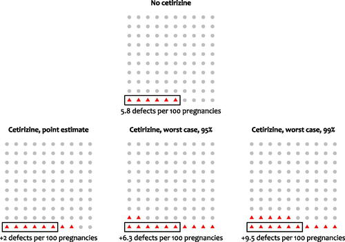
Fitting a classical logistic model with the binary birth defect outcome predicted from the cetirizine indicator confirmed the nonsignificant relationship (p = 0.287). The point estimate of the effect of taking cetirizine is to increase the odds of the birth defect by only 37%. At the baseline levels of birth defects in the non-cetirizine-exposed sample (approximately 6%), this would amount to about an extra two birth defects in every hundred pregnancies in the cetirizine-exposed group.

There are several problems with taking these data as evidence that cetirizine is safe. The first is the observational nature of the data. We have no way of knowing whether an apparent effect—or lack of effect—reflects confounds. Suppose, though, that we set this question aside and assess the evidence that birth defects are not more common in the cetirizine group. We can use a classical one-sided CI to determine the size of the differences we can rule out. We call the upper bound of the 100($1-\alpha$)% CI the “worst case” for that confidence coefficient. Figure 1 shows that at 95%, the worst-case odds increase is for the cetirizine group is 124%. At 99.5%, the worst case increase is 195%. We can translate this into more a more intuitive metric of numbers of birth defects: at baseline rates of birth defects, these would amount to additional 6 and 10 birth defects per 100, respectively (Figure 2).

Fig. 1 Estimates of the odds of a birth defect when no cetirizine (control) was taken during pregnancy and when cetirizine was taken. Horizontal dashed lines and shaded regions show point estimates and standard errors. The solid line labeled “Cetirizine worst case” shows the upper bound of the one-sided CI as a function of the confidence coefficient (x-axis). The right axis shows the estimated increase in odds of a birth defect for the cetirizine group compared to the control group.

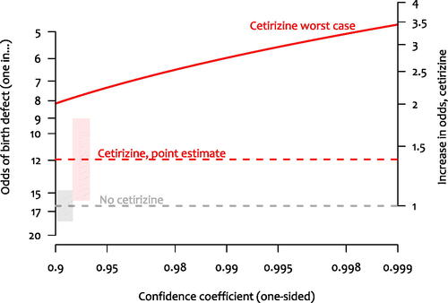
Fig. 2 Frequency representations of the number of birth defects expected under various scenarios. Top: Expected frequency of birth defects when cetirizine was not taken (control). Bottom-left: Point estimate of the expected frequency of birth defects when cetirizine is taken. Bottom-middle (bottom-right): Upper bound of a one-sided 95% (99%) CI for the expected frequency of birth defects when cetirizine was taken. Because the analysis is intended to be comparative, in the bottom panels the no-cetirizine estimate was assumed to be the truth when calculating the increase in frequency.

The large p-value of the initial significance test suggests that we cannot rule out that cetirizine group has lower rates of birth defects; the one-sided test assuming a decrease in birth defects as the null would not yield a rejection except at high α levels. But also, the “worst-case” analysis using the upper bound of the one-sided CI suggests we also cannot rule out a substantial increase in birth defects in the cetirizine group.

We are unsure whether cetirizine is safe, but it seems clear to us that these data do not provide much evidence of its relative safety, contrary to what Weber-Schoendorfer and Schaefer suggest.

2.5 Analysis and Interpretation by Gronau, van Doorn, and Wagenmakers

We used the model proposed by Kass and Vaidyanathan (1992):$$\begin{array}{cc}\hfill & \hspace{0.17em}\text{log}\hspace{0.17em}\left(\frac{p_1}{1-p_1}\right)=\beta -\frac{\psi }{2},\hfill \\ \hfill & \hspace{0.17em}\text{log}\hspace{0.17em}\left(\frac{p_2}{1-p_2}\right)=\beta +\frac{\psi }{2},\hfill \\ \hfill & y_1\sim \text{Binomial}(n_1,p_1),\hfill \\ \hfill & y_2\sim \text{Binomial}(n_2,p_2).\hfill \end{array}$$

Here, $y_1=97,n_1=1,685,y_2=14$, and $n_2=181$, p₁ is the probability of a birth defect in the control group, and p₂ is that probability in the cetirizine group. Probabilities p₁ and p₂ are functions of model parameters β and ψ. Nuisance parameter β corresponds to the grand mean of the log odds, whereas the test-relevant parameter ψ corresponds to the log odds ratio. We assigned β a standard normal prior and used a zero-centred normal prior with standard deviation σ for the log odds ratio ψ. Inference was conducted with Stan (Carpenter et al. 2017; Stan Development Team 2016) and the bridgesampling package (Gronau, Singmann, and Wagenmakers in press). For ease of interpretation, the results will be shown on the odds ratio scale.

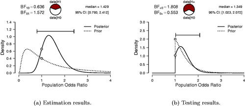
Our first analysis focuses on estimation and uses σ = 1. The result, shown in the left panel of Figure 3, indicates that the posterior median equals 1.429, with a 95% credible interval ranging from 0.793 to 2.412. This credible interval is relatively wide, indicating substantial uncertainty about the true value of the odds ratio.

Fig. 3 Gronau, van Doorn, and Wagenmakers’ Bayesian analysis of the cetirizine dataset. The left panel shows the results of estimating the log odds ratio under ${\mathcal{H}}_1$ with a two-sided standard normal prior. For ease of interpretation, results are displayed in the odds ratio scale. The right panel shows the results of testing the one-sided alternative hypothesis ${\mathcal{H}}_{+}:\psi \sim {\mathcal{N}}^{+}(0,{0.4}^2)$ versus the null hypothesis ${\mathcal{H}}_0:\psi =0$. Figures inspired by JASP (jasp-stats.org).

Our second analysis focuses on testing and quantifies the extent to which the data support the skeptic’s ${\mathcal{H}}_0:\psi =0$ versus the proponent’s ${\mathcal{H}}_1$. To specify ${\mathcal{H}}_1$ we initially use $\sigma =0.4$ (i.e., a mildly informative prior; Diamond and Kaul 2004), truncated at zero to respect the fact that cetirizine exposure is hypothesized to cause a higher incidence of birth defects: ${\mathcal{H}}_{+}:\psi \sim N^{+}(0,{0.4}^2)$.

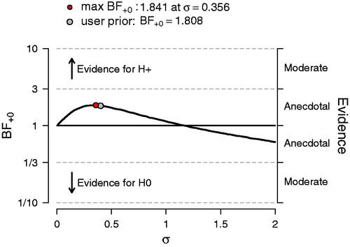
As can be seen from the right panel of Figure 3, the observed data are predicted about 1.8 times better by ${\mathcal{H}}_{+}$ than by ${\mathcal{H}}_0$. According to Jeffreys (1961, Appendix B), this level of support is “not worth more than a bare mention.” To investigate the robustness of this result, we explored a range of alternative prior choices for σ under ${\mathcal{H}}_{+}$, varying it from 0.01 to 2. The results of this sensitivity analysis are shown in Figure 4 and reveal that across a wide range of priors, the data never provide more than anecdotal support for one model over the other. When σ is selected post hoc to maximize the support for ${\mathcal{H}}_{+}$ this yields ${\text{BF}}_{+0}=1.84$, which, starting from a position of equipoise, raises the probability of ${\mathcal{H}}_{+}$ from 0.50 to about 0.65, leaving a posterior probability of 0.35 for ${\mathcal{H}}_0$.

Fig. 4 Sensitivity analysis for the Bayesian one-sided test. The Bayes factor ${\text{BF}}_{+0}$ is a function of the prior standard deviation σ. Figure inspired by JASP.

In sum, based on this dataset we cannot draw strong conclusions about whether or not cetirizine exposure during pregnancy is associated with a higher incidence of birth defects. Our analysis shows an “absence of evidence,” not “evidence for absence.”

2.6 Analysis and interpretation by Gelman

I summarized the data with a simple comparison: the proportion of birth defects is 0.06 in the control group and 0.08 in the cetirizine group. The difference is 0.02 with a standard error of 0.02. I got essentially the same result with a logistic regression predicting birth defect: the coefficient of cetirizine is 0.3 with a standard error of 0.3. I performed the analyses in R using rstanarm (code available at https://osf.io/nh4gc/).

I then looked up the article, “The safety of cetirizine during pregnancy: A prospective observational cohort study,” by Weber-Schoendorfer and Schaefer (2008) and noticed some interesting things:

1. The published article gives N = 196 and 1686 for the two groups, not quite the same as the 181 and 1685 for the “all birth defects” category. I could not follow the exact reasoning.⁴

2. The two groups differ in various background variables: most notably, the cetirizine group has a higher smoking rate (17% compared to 10%).

3. In the published article, the outcome of focus was “major birth defects,” not the “all birth defects” given for us to study.

4. The published article has a causal aim (as can be seen, for example, from the word “safety” in its title); our assignment is purely observational.

Now the question, “Is cetirizine exposure during pregnancy associated with a higher incidence of birth defects?” I have not read the literature on the topic. To understand how the data at hand address this question, I would like to think of the mapping from prior to posterior distribution. In this case, the prior would be the distribution of association with birth defects of all drugs of this sort. That is, imagine a population of drugs, $j=1,2,\dots$, taken by pregnant women, and for each drug, define θ_j as the proportion of birth defects among women who took drug j, minus the proportion of birth defects in the general population. Just based on my general understanding (which could be wrong), I would expect this distribution to be more positive than negative and concentrated near zero: some drugs could be mildly protective against birth defects or associated with low-risk pregnancies, most would have small effects and not be strongly associated with low- or high-risk pregnancies, and some could cause birth defects or be taken disproportionately by women with high-risk pregnancies. Supposing that the prior is concentrated within the range (–0.01, + 0.01), the data would not add much information to this prior.

To answer, “Is cetirizine exposure during pregnancy associated with a higher incidence of birth defects?,” the key question would seem to be whether the drug is more or less likely to be taken by women at a higher risk of birth defects. I am guessing that maternal age is a big predictor here. In the reported study, average age of the exposed and control groups was the same, but I do not know if that is generally the case or if the designers of the study were purposely seeking a balanced comparison.

3 DataSet II: Amygdalar Activity and Perceived Stress

3.1 Study Summary

In a recent study published in the Lancet, Tawakol et al. (2017) tested the hypothesis that perceived stress is positively associated with resting activity in the amygdala. In the second study reported in Tawakol et al. (2017), n = 13 individuals with an increased burden of chronic stress (i.e., a history of posttraumatic stress disorder or PTSD) were recruited from the community, completed a Perceived Stress Scale (i.e., the PSS-10; Cohen, Kamarck, and Mermelstein 1983) and had their amygdalar activity measured. Variables of the dataset⁵ are described in Table 3, the raw data are presented in Table 4, and the data are visualized in Figure 5.

Fig. 5 Scatterplot of amygdalar activity and perceived stress in 13 patients with PTSD. Data extracted from Figure 5 in Tawakol et al. (2017), with help of Jurgen Rusch, Philips Research Eindhoven.

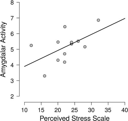
Table 3 Variable names and their description.

Variable	Description
Perceived stress scale	Participant score on the PSS
Amygdalar activity	Intensity of amygdalar resting state activity

Table 4 Raw data as extracted from Figure 5 in Tawakol et al. (2017), with help of Jurgen Rusch, Philips Research Eindhoven.

Perceived	Amygdalar
Stress Scale	Activity
12.0103	5.2418
32.0350	6.8601
22.0296	6.4402
20.0079	5.4620
24.0155	5.4439
24.0155	5.3349
24.0155	5.4216
26.0082	5.5176
28.0120	5.1615
21.9872	4.7114
21.9872	4.1844
20.0138	4.3079
16.0088	3.3015

3.2 Amygdala Research Question

Do PTSD patients with high resting state amygdalar activity experience more stress? In the next sections each of four data analysis teams will attempt to address this question.

3.3 Analysis and Interpretation by Lakens and Hennig

3.3.1 Analysis and Software

We calculated tests for uncorrelatedness based on both Pearson’s product-moment correlation and Spearman’s rank correlation using the cor.test function in the stats package in R 3.4.3.

3.3.2 Results and interpretation

The Pearson correlation between perceived stress and resting activity in the amygdala is r = 0.555, and the corresponding test yields $p=0.047$. Although this is just smaller than the conventional 5% level, we do not consider it as clear evidence for nonzero correlation. From the appendix it becomes clear that the reported correlations are exploratory: “Patients completed a battery of self-report measures that assessed variables that may correlate with PTSD symptom severity, including comorbid depressive and anxiety symptoms (MADRS, HAMA) and a well-validated questionnaire Perceived Stress Scale (PSS-10).” Therefore, corrections for multiple comparisons would be required to maintain a given significance level. The article does not provide us with sufficient information to determine the number of tests that were performed, but corrections for multiple comparisons would thus be in order. Consequently, the fairly large observed correlation and the borderline significant p-value can be interpreted as an indication that it may be worthwhile to investigate the issue with a larger sample size, but do not give conclusive evidence. Visual inspection of the data does not give any indication against the validity of using Pearson’s correlation, but with N = 13 we do not have very strong information regarding the distributional shape. The analogous test based on Spearman’s correlation yields $p=0.062$, which given its weaker power is compatible with the qualitative interpretation we gave based on the Pearson correlation.

Do PTSD patients with high resting state amygdalar activity experience more stress? Based on the current study, we cannot conclude that PTSD patients with high resting state amygdalar activity experience more stress. The single p = 0.047 is not low enough to indicate clear evidence against the null hypothesis after correcting for multiple comparisons when using an alpha of 0.05. Therefore, our conclusion is: Based on the desired error rate specified by the authors, we cannot reject a correlation of zero between amygdalar activity and participants’ score on the perceived stress scale. With a 95% CI that ranges from r = 0 to r = 0.85, it seems clear that effects that would be considered interesting cannot be rejected in an equivalence test. Thus, the results are inconclusive.

3.4 Analysis and Interpretation by Morey and Homer

The first thing that should be noted about this dataset is that it contains a meager 13 data points. The linear correlation by Tawakol et al. (2017) depends on assumptions that are for all intents and purposes unverifiable with this few participants. Add to this the difficulty of interpreting the independent variable—a sum of ordinal responses—and we are justified being skeptical of any hard conclusions from these data.

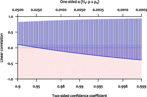
Suppose, however, that the relationship between these two variables was best characterized by a linear correlation, and set aside any worries about assumptions. The large observed correlation coupled with the marginal p-value should signal to us that a wide range of correlations are not ruled out by the data. Consider that the 95% CI on the Pearson correlation is [0.009,0.848]; the 99.5% CI is [–0.254,0.908]. Negligible correlations are not ruled out; due to the small sample size, any correlation from “essentially zero” to “the correlation between height and leg length” (i.e., very high) is consistent with these data. The solid curve in Figure 6 shows the lower bound of the confidence interval on the linear correlation for a wide range of confidence levels; they are all negligible or even negative.

Fig. 6 Confidence intervals and one-sided tests for the Pearson correlation as a function of the confidence coefficient. The vertical lines represent the confidence intervals (confidence coefficient on lower axis), and the curve represents the value that is just rejected by the one-sided test (α on the upper axis).

Finally, the authors did not show that this correlation is selective to the amygdala; it seems to us that interpreting the correlation as evidence for their model requires selectivity. It is important to interpret the correlation in the context of the relationship between amygdala resting state activity, stress, and cardiovascular disease. If one could not show that amygdala resting-state activation showed a substantially higher correlation with stress than other brain regions not implicated in the model, this would suggest that the correlation cannot be used to bolster their case. Given the uncertainty in the estimate of the correlation, there is little chance of being able to show this.

All in all, we are not sure that the information in these thirteen participants is enough to say anything beyond “the correlation doesn’t appear to be (very) negative.”

3.5 Analysis and Interpretation by Van Doorn, Gronau, and Wagenmakers

We applied Harold Jeffreys’s test for a Pearson correlation coefficient ρ (Jeffreys 1961; Ly, Marsman, and Wagenmakers 2018) as implemented in JASP (jasp-stats.org; JASP Team 2018).⁶ Our first analysis focuses on estimation and assigns ρ a uniform prior from –1 to 1. The result, shown in the left panel of Figure 7, indicates that the posterior median equals 0.47, with a 95% credible interval ranging from –0.01 to 0.81. As can be expected with only 13 observations, there is great uncertainty about the size of ρ.

Fig. 7 van Doorn, Gronau, and Wagenmakers’ Bayesian analysis of the amygdala dataset. The left panel shows the result of estimating the Pearson correlation coefficient ρ under ${\mathcal{H}}_1$ with a two-sided uniform prior. The right panel shows the result of testing ${\mathcal{H}}_0:\rho =0$ versus the one-sided alternative hypothesis ${\mathcal{H}}_{+}:\rho \sim U[0,1]$. Figures from JASP.

Our second analysis focuses on testing and quantifies the extent to which the data support the skeptic’s ${\mathcal{H}}_0:\rho =0$ versus the proponent’s ${\mathcal{H}}_1$. To specify ${\mathcal{H}}_1$, we initially use Jeffreys’s default uniform distribution, truncated at zero to respect the directionality of the hypothesized effect: ${\mathcal{H}}_{+}:\rho \sim U[0,1]$.

As can be seen from the right panel of Figure 7, the observed data are predicted about 3.9 times better by ${\mathcal{H}}_{+}$ than by ${\mathcal{H}}_0$. This degree of support is relatively modest: when ${\mathcal{H}}_{+}$ and ${\mathcal{H}}_0$ are equally likely a priori, the Bayes factor of 3.9 raises the posterior plausibility of ${\mathcal{H}}_{+}$ from 0.50 to 0.80, leaving a nonnegligible 0.20 for ${\mathcal{H}}_0$.

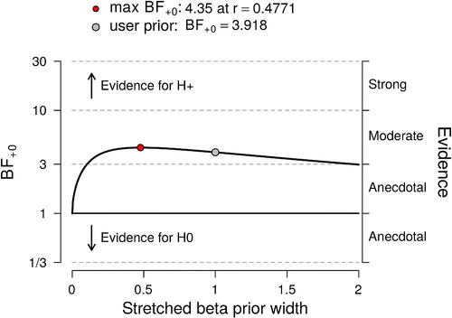
To investigate the robustness of this result, we explored a continuous range of alternative prior distributions for ρ under ${\mathcal{H}}_{+}$; specifically, we assigned ρ a stretched Beta(a,a) distribution truncated at zero, and studied how the Bayes factor changes with $1/a$, the parameter that quantifies the prior width and governs the extent to which ${\mathcal{H}}_{+}$ predicts large values of r. The results of this sensitivity analysis are shown in Figure 8 and confirm that the data provide modest support for ${\mathcal{H}}_{+}$ across a wide range of priors. When the precision is selected post hoc to maximize the support for ${\mathcal{H}}_{+}$ this yields ${\text{BF}}_{+0}=4.35$, which—under a position of equipose– raises the plausibility of ${\mathcal{H}}_{+}$ from 0.50 to about 0.81, leaving a posterior probability of 0.19 for ${\mathcal{H}}_0$.

Fig. 8 Sensitivity analysis for the Bayesian one-sided correlation test. The Bayes factor ${\text{BF}}_{+0}$ is a function of the prior width parameter $1/a$ from the stretched Beta(a,a) distribution. Figure from JASP.

A similar sensitivity analysis could be conducted for ${\mathcal{H}}_0$ by assuming a “perinull” (Tukey 1995, p. 8)—a distribution tightly centered around ρ = 0 rather than a point mass on ρ = 0. The results will be qualitatively similar.

In sum, the claim that “PTSD patients with high resting state amygdalar activity experience more stress” receives modest but not compelling support from the data.” The 13 observations do not warrant categorical statements, neither about the presence nor about the strength of the hypothesized effect.

3.6 Analysis and interpretation by Gelman

I summarized the data with a simple scatterplot and a linear regression of logarithm of perceived stress on logarithm of amygdalar activity, using log scales because the data were all-positive and it seemed reasonable to model a multiplicative relation. The scatterplot revealed a positive correlation and no other striking patterns, and the regression coefficient was estimated at 0.6 with a standard error of 0.4. I performed the analyses in R using rstanarm (code available at https://osf.io/nh4gc/). and the standard error is based on the median absolute deviation of posterior simulations (see help(“mad”) in R for more on this).

I then looked up the article, “Relation between resting amygdalar activity and cardiovascular events: a longitudinal and cohort study,” by Tawakol et al. (2017). The goal of the research is “to determine whether [the amygdala’s] resting metabolic activity predicts risk of subsequent cardiovascular events.” Here are some items relevant to our current task:

1. Perceived stress is an intermediate outcome, not the ultimate goal of the study.

2. Any correlation or predictive relation will depend on the reference population. The people in this particular study are “individuals with a history of posttraumatic stress disorder” living in the Boston area.

3. The published article reports that “Perceived stress was associated with amygdalar activity (r = 0.56; p = 0.0485).” Performing the correlation (or, equivalently, the regression) on the log scale, the result is not statistically significant at the 5% level. This is no big deal given that I do not think that it makes sense to make decisions based on a statistical significance threshold, but it is relevant when considering scientific communication.

4. Comparing my log-scale scatterplot to the raw-scale scatterplot (Figure 5A in the published article), I would say that the unlogged scatterplot looks cleaner, with the points more symmetrically distributed. Indeed, based on these data alone, I would move to an unlogged analysis–that is, the estimated correlation of 0.56 reported in the article.

To address the question, “Do PTSD patients with high resting state amygdalar activity experience more stress?,” we need two additional decisions or pieces of information. First, we must decide the population of interest; here there is a challenge in extrapolating from people with PTSD to the general population. Second, we need a prior distribution for the correlation being estimated. It is difficult for me to address either of these issues: as a statistician my contribution would be to map from assumptions to conclusions. In this case, the assumptions about the prior distribution and the assumptions about extrapolation go together, as in both cases we need some sense of how likely it is to see large correlations between the responses to a subjective stress survey and a biomeasurement such as amygdalar activity. It could well be that there is a prior expectation of positive correlation between these two variables in the general population, but that the current data do not provide much information beyond our prior for this general question.

4 Round-Table Discussion

As described above, the two datasets have each been analyzed by four teams. The different approaches and conclusions are summarized in Table 5. The discussion was carried out via E-mail and a transcript can be found online at https://osf.io/f4z7x/. Below we highlight and summarize the central elements of a discussion that quickly proceeded from the data analysis techniques in the concrete case to more fundamental philosophical issues. Given the relative agreement among the conclusions reached by different methodological angles, our discussion started out with the following deliberately provocative statement:

Table 5 Overview of the approaches and results of the research teams.

Research team	DataSet I: Cetirizine and birth defects	DataSet II:Amygdalar Activity
Lakens and Hennig	Frequentist test of equivalence 10% equivalence region Data deemed inconclusive	Frequentist correlation, p =.047 Concerns about multiple comparisons Data deemed inconclusive
Morey and Homer	Frequentist logistic model, p =.287 Observational, so possible confounds Data deemed inconclusive	Frequentist correlation, $p=.047$ Small n means assumptions unverifiable Is the effect specific for amygdala? Data deemed inconclusive
Gronau, Van Doorn, and Wagenmakers	Default Bayes factor ${\text{BF}}_{01}=1.6$ Evidence “not worth more than a bare mention” Data deemed inconclusive	Default Bayes factor ${\text{BF}}_{10}=2$ Small n Data deemed inconclusive
Gelman	Bayesian analysis needs good prior Data likely to be inconclusive A key question is who takes the drug in the population	Bayesian analysis needs good prior Problems with generalizing to population Data likely to be inconclusive

In statistics, it doesn’t matter what approach is used. As long as you do conduct your analysis with care, you will invariably arrive at the same qualitative conclusion.⁷

In agreement with this claim, Hennig stated that “we all seem to have a healthy skepticism about the models that we are using. This probably contributes strongly to the fact that all our final interpretations by and large agree. Ultimately our conclusions all state that “the data are inconclusive.” I think the important point here is that we all treat our models as tools for thinking that can only do so much, and of which the limitations need to be explored, rather than ‘believing in’ our relying on any specific model (Email 29). On the other hand, Hennig wonders “whether differences between us would’ve been more pronounced with data that wouldn’t have allowed us to sit on the fence that easily” (Email 29) and Lakens wonders “about what would have happened if the data were clearer” (Email 32). In addition, Morey points out that “none of us had anything invested in these questions, whereas almost always analyses are published by people who are most invested” (Email 33). Wagenmakers responds that we [referring to the group that organized this study] wanted to use simple problems that would not pose immediate problems for either one of the paradigms…[and] we tried to avoid data sets that met Berkson’s ‘inter-ocular traumatic test’ (when the data are so clear that the conclusion hits you right between the eyes) where we would immediately agree. (Email 31).

Moreover, the focus was on the analyses and discussion as free as possible from other consideration (e.g., personal investment in the questions).

However, differences between the analyses were emphasized as well. First, Morey argued that the differences (e.g., research planning, execution, analysis, etc.) between the Bayesian and frequentist approach are critically important and not easily inter-translatable (Email 2). This gave rise to an extended discussion about the frequentist procedures’ dependence of the sampling protocol, which Bayesian procedures lack. While Bayesians such as Wagenmakers see this as a critical objection against the coherent use of frequentist procedures (e.g., in cases where the sampling protocol is uncertain), Hennig contends that one can still interpret the p-value as indicating the compatibility of the data with the null model, assuming a hypothetical sampling plan (see Email 5–11, 16–18, 23, and 24). Second, Lakens speculated that, in the cases where the approaches differ, there “might be more variation within specific approaches, than between” (Email 1). Third, Hennig pointed out that differences in prior specifications could lead to discrepancies between Bayesians (Email 4) and Homer pointed out that differences in alpha decision boundaries could lead to discrepancies between frequentists’ conclusions (Email 11). Finally, Gelman disagreed with most of what had been said in the discussion thus far. Specifically, he said: “I don’t think ‘alpha’ makes any sense, I don’t think 95% intervals are generally a good idea, I don’t think it’s necessarily true that points in 95% interval are compatible with the data, etc etc.” (Email 15).

A concrete issue concerned the equivalence test used by Lakens and Hennig for the first dataset. Wagenmakers objects that it does not add relevant information to the presentation of a confidence interval (Email 12). Lakens responds that it allows to reject the hypothesis of a >10% difference in proportions at almost any alpha level, thereby avoiding reliance on default alpha levels, which are often used in a mindless way and without attention to the particular case (Email 13).

A more foundational point of contention with the two datasets and their analysis was about the question of how to formulate Bayesian priors. For these concrete cases, Hennig contends that the subject-matter information cannot be smoothly translated into prior specifications (Email 27), which is the reason why Morey and Homer choose a frequentist approach, while Gelman considers it “hard for me to imagine how to answer the questions without thinking about subject-matter information” (Email 26).

Lakens raised the question of how much the approaches in this paper are representative of what researchers do in general (Email 43 and 44). Wagenmakers’ discussion of p-values echoes this point. While Lakens describes p-values as a guide to “deciding to act in a certain way with an acceptable risk of error” and contends many scientists conform to this rationale (Email 32), Wagenmakers has a more pessimistic view. In his experience, the role of p-values is less epistemic than social: they are used to convince referees and editors and to suggest that the hypothesis in question is true (Email 37). Also Hennig disagrees with Lakens, but from a frequentist point of view: p-values should not guide binary accept/reject-decisions, they just indicate the degree to which the observed data is compatible with the model specified by the null hypothesis (Email 34).

The question of how data analysis relates to learning, inference and decision making was also discussed regarding the merits (and problems) of Bayesian statistics. Hennig contends that there can be “some substantial gain from them [priors] only if the prior encodes some relevant information that can help the analysis. However, here we don’t have such information” and the Bayesian “approach added unnecessary complexity” (Email 23). Wagenmakers reply is that “the prior is not there to help or hurt an analysis: it is there because without it, the models do not make predictions; and without making predictions, the hypotheses or parameters cannot be evaluated” and that “the approach is more complex, but this is because it includes some essential ingredients that the classical analysis omits” (Email 24). In fact, he insinuates that frequentists learn from data through “Bayes by stealth”: the observed p-values, confidence intervals and other quantities are used to update the plausibility of the models in an “inexact and intuitive” way. “Without invoking Bayes’ rule (by stealth) you can’t learn much from a classical analysis, at least not in any formal sense.” (Email 24) According to Hennig, there is more to learning than “updating epistemic probabilities of certain parameter values being true. For example I find it informative to learn that ‘Model X is compatible with the data’” (Email 25). However, Wagenmakers considers Hennig’s example of learning as a synonymous to observing. Though he agrees that “it is informative to know when a specific model is or is not compatible with data; to learn anything, however, by its very definition requires some form of knowledge updating” (Email 30). This discussion evolved, finally, into a general discussion about the philosophical principles and ideas underlying schools of statistical inference. Ironically, both Lakens (decision-theoretically oriented frequentism) and Gelman (falsificationist Bayesianism) claim the philosophers of science Karl Popper and Imre Lakatos, known for their ideas of accumulating scientific progress through successive falsification attempts, as one of their primary inspirations, although they spell out their ideas in a different way (Email 42 and 45).

Hennig and Lakens also devoted some attention to improving statistical practice and either directly or indirectly questioned the relevance of foundational debates. Concerning the above issue with using p-values for binary decision making, Hennig suspects that “if Bayesian methodology would be in more widespread use, we’d see the same issue there… and then ‘reject’ or ‘accept’ based on whether a posterior probability is larger than some mechanical cutoff” (Email 34) and “that much of the controversy about these approaches concerns naive ‘mechanical’ applications in which formal assumptions are taken for granted to be fulfilled in reality” (Email 29). In addition, Lakens points out thatwhether you use one approach to statistics or another doesn’t matter anything in practice. If my entire department would use a different approach to statistical inferences (now everyone uses frequentist hypothesis testing) it would have basically zero impact on their work. However, if they would learn how to better use statistics, and apply it in a more thoughtful manner, a lot would be gained. (Email 32)

Homer provides an apt conclusion to this topic by stating “I think a lot of problems with research happen long before statistics get involved. E.g. Issues with measurement; samples and/or methods that can’t answer the research question; untrained or poor observers” (Email 35).

Finally, an interesting distinction was made between a prescriptive use of statistics and a more pragmatic use of statistics. As an illustration of the latter, Hennig has a more pragmatic perspective on statistics, because a strong prescriptive view (i.e., fulfillment of modeling assumptions as a strict requirement for statistical inference) would often mean that we can’t do anything in practice (Email 2). To clarify this point, he adds: “Model assumptions are never literally fulfilled so the question cannot be whether they are…, but rather whether there is information or features of the data that will mislead the methods that we want to apply” (Email 23). The former is illustrated by Homer:

I think that assumptions are critically important in statistical analysis. Statistical assumptions are the axioms which allow a flow of mathematical logic to lead to a statistical inference. There is some wiggle room when it comes to things like ‘how robust is this test, which assumes normality, to skew?’ but you are on far safer ground when all the assumptions are/appear to be met. I personally think that not even checking the plausibility of assumptions is inexcusable sloppiness (not that I feel anyone here suggested otherwise). (Email 11)

From what has been said in the discussion, there is general consensus that not all assumptions need to be met and not all rules need to be strictly followed. However, there is great disagreement about which assumptions are important; which rules should be followed and how strictly; and what can be interpreted from the results when (it is uncertain if) these rules and assumptions are violated. The interesting subtleties of this topic and the discussants’ views on use of statistics can be read in the online supplement (model assumptions: Email 4, 11, 23, and 24; alpha-levels, p-values, Bayes factors, and decision procedures: Email 2, 9, 11, 14, 15, 24, and 31–40; sampling plan, optional stopping, and conditioning on the data: Email 2, 5–11, 16–18, 23, and 24).

In summary, dissimilar methods were used that resulted in similar conclusions and varying views were discussed on how statistical methods are used and should be used. At times it was a heated debate with interesting arguments from both (or more) sides. As one might expect, there was disagreement about particularities of procedures and consensus on the expectation that scientific practice would be improved by better general education on the use of statistics.

5 Closing Remarks

Four teams each analyzed two published datasets. Despite substantial variation in the statistical approaches employed, all teams agreed that it would be premature to draw strong conclusions from either of the datasets. Adding to this cautious attitude are concerns about the nature of the data. For instance, the first dataset was observational, and the second dataset may require a correction for multiplicity. In addition, for each scenario, the research teams indicated that more background information was desired; for instance, “when is the difference in birth defects considered too small to matter?”; “what are the effects for similar drugs?”; “is the correlation selective to the amygdala?”; and “what is the prior distribution for the correlation?”. Unfortunately, in the routine use of statistical procedures such information is provided only rarely.

It also became evident that the analysis teams not only needed to make assumptions about the nature of the data and any relevant background knowledge, but they also needed to interpret the research question. For the first dataset, for instance, the question was formulated as “Is cetirizine exposure during pregnancy associated with a higher incidence of birth defects?”. What the original researchers wanted to know, however, is whether or not cetirizine is safe—this more general question opens up the possibility of applying alternative approaches, such as the equivalence test, or even a statistical decision analysis: should pregnant women be advised not to take cetirizine? We purposefully tried to steer clear from decision analyses because the context-dependent specification of utilities adds another layer of complexity and requires even more background knowledge than was already demanded for the present approaches. More generally, the formulation of our research questions was susceptible to multiple interpretation: as tests against a point null, as tests of direction, or as tests of effect size. The goals of a statistical analysis can be many, and it is important to define them unambiguously—again, the routine use of statistical procedures almost never conveys this information.

Despite the (unfortunately near-universal) ambiguity about the nature of the data, the background knowledge, and the research question, each analysis team added valuable insights and ideas. This reinforces the idea that a careful statistical analysis, even for the simplest of scenarios, requires more than a mechanical application of a set of rules; a careful analysis is a process that involves both skepticism and creativity. Perhaps popular opinion is correct, and statistics is difficult. On the other hand, despite employing widely different approaches, all teams nevertheless arrived at a similar conclusion. This tentatively supports the Fisher–Jeffreys conjecture that, regardless of the statistical framework in which they operate, careful analysts will often come to similar conclusions.

Notes

Additional information

Funding

This work was supported in part by a Vici grant from the Netherlands Organisation of Scientific Research awarded to EJW (016.Vici.170.083) and a Vidi grant awarded to DL (452.17.013). NvD’s and JS’s work was supported by ERC Starting Investigator Grant No. 640638.

Notes

1 In contrast to the current approach, Silberzahn et al. (in press) used a relatively complex dataset and did not emphasize the differences in interpretation caused by the adoption of dissimilar statistical paradigms.

2 The original study focused on cetirizine-induced differences in major birth defects, spontaneous abortions, and preterm deliveries. We decided to look at all birth defects, because the sample sizes were larger for this comparison and we deemed the data more interesting.

3 The dataset is made available on the OSF repository: https://osf.io/hykmz/.

4 Clarification: the original article does not provide a rationale for why several participants were excluded from the analysis.

5 The dataset is made available on the OSF repository: https://osf.io/hykmz/.

6 JASP is an open-source statistical software program with a graphical user interface that supports both frequentist and Bayesian analyses.

7 The statement is based on Jeffreys’ claims “[a]s a matter of fact I have applied my significance tests to numerous applications that have also been worked out by Fisher’s, and have not yet found a disagreement in the actual decisions reached” (Jeffreys 1939, p. 365) and “it would only be once in a blue moon that we [Fisher and Jeffreys] would disagree about the inference to be drawn in any particular case, and that in the exceptional cases we would both be a bit doubtful” (Bennett 1990, p. 162).

References

- Benjamin, D. J., Berger, J. O., Johannesson, M., Nosek, B. A., Wagenmakers, E.-J., Berk, R., Bollen, K. A., Brembs, B., Brown, L., Camerer, C., Cesarini, D., Chambers, C. D., Clyde, M., Cook, T. D., De Boeck, P., Dienes, Z., Dreber, A., Easwaran, K., Efferson, C., Fehr, E., Fidler, F., Field, A. P., Forster, M., George, E. I., Gonzalez, R., Goodman, S., Green, E., Green, D. P., Greenwald, A., Hadfield, J. D., Hedges, L. V., Held, L., Ho, T.-H., Hoijtink, H., Jones, J. H., Hruschka, D. J., Imai, K., Imbens, G., Ioannidis, J. P. A., Jeon, M., Kirchler, M., Laibson, D., List, J., Little, R., Lupia, A., Machery, E., Maxwell, S. E., McCarthy, M., Moore, D., Morgan, S. L., Munafò, M., Nakagawa, S., Nyhan, B., Parker, T. H., Pericchi, L., Perugini, M., Rouder, J., Rousseau, J., Savalei, V., Schönbrodt, F. D., Sellke, T., Sinclair, B., Tingley, D., Van Zandt, T., Vazire, S., Watts, D. J., Winship, C., Wolpert, R. L., Xie, Y., Young, C., Zinman, J., and Johnson, V. E. (2018), “Redefine Statistical Significance.” Nature Human Behaviour, 2:6–10. DOI: 10.1038/s41562-017-0189-z.
- Bennett, J. H., editor (1990), Statistical Inference and Analysis: Selected Correspondence of R. A. Fisher. Clarendon Press, Oxford.
- Berger, J. O. (2003), “Could Fisher, Jeffreys and Neyman Have Agreed on Testing?” Statistical Science, 18:1–32. DOI: 10.1214/ss/1056397485.
- Carpenter, B., Gelman, A., Hoffman, M., Lee, D., Goodrich, B., Betancourt, M., Brubaker, M., Guo, J., Li, P., and Riddell, A. (2017). “Stan: A probabilistic Programming Language.” Journal of Statistical Software, 76:1–32.
- Chen, J. J., Tsong, Y., and Kang, S.-H. (2000), “Tests for Equivalence or Noninferiority Between Two Proportions.” Drug Information Journal, 26:569–578. DOI: 10.1177/009286150003400225.
- Cohen, S., Kamarck, T., and Mermelstein, R. (1983), “A Global Measure of Perceived Stress.” Journal of Health and Social Behavior, 24:385–396.
- Diamond, G. A., and Kaul, S. (2004), “Prior Convictions: Bayesian Approaches to the Analysis and Interpretation of Clinical Megatrials,” Journal of the American College of Cardiology, 43:1929–1939. DOI: 10.1016/j.jacc.2004.01.035.
- Edwards, W., Lindman, H., and Savage, L. J. (1963), “Bayesian Statistical Inference for Psychological Research,” Psychological Review, 70:193–242. DOI: 10.1037/h0044139.
- Efron, B. (1986), “Why Isn’t Everyone a Bayesian?” The American Statistician, 40:1–5. DOI: 10.2307/2683105.
- Gronau, Q. F., Singmann, H., and Wagenmakers, E.-J. (in press), “Bridgesampling: An R Package for Estimating Normalizing Constants,” Journal of Statistical Software.
- Howie, D. (2002). Interpreting Probability: Controversies and Developments in the Early Twentieth Century. Cambridge: Cambridge University Press. DOI: 10.1163/182539104X00304.
- JASP Team (2018). JASP (Version 0.9)[Computer software].
- Jeffreys, H. (1939). Theory of Probability (1st ed.). Oxford: Oxford University Press.
- Jeffreys, H. (1961). Theory of Probability (3rd ed.). Oxford: Oxford University Press.
- Kass, R. E., and Vaidyanathan, S. K. (1992), “Approximate Bayes Factors and Orthogonal Parameters, With Application to Testing Equality of Two Binomial Proportions,” Journal of the Royal Statistical Society, Series B, 54:129–144. DOI: 10.1111/j.2517-6161.1992.tb01868.x.
- Lakens, D. (2017), “Equivalence Tests: A Practical Primer for t Tests, Correlations, and Meta-analyses,” Social Psychological and Personality Science, 8:355–362. DOI: 10.1177/1948550617697177.
- Lindley, D. V. (1986). “Comment on ‘Why Isn’t Everyone a Bayesian?’ By Bradley Efron.” The American Statistician, 40:6–7.
- Ly, A., Marsman, M., and Wagenmakers, E.-J. (2018), “Analytic Posteriors for Pearson’s Correlation Coefficient,” Statistica Neerlandica, 72:4–13. DOI: 10.1111/stan.12111.
- McShane, B. B., Gal, D., Gelman, A., Robert, C., and Tackett, J. L. (in press), “Abandon Statistical Significance,” The American Statistician.
- R Development Core Team (2004). R: A Language and Environment for Statistical Computing, Vienna, Austria: R Foundation for Statistical Computing. ISBN 3–900051–00–3.
- Röhmel, J. (2001), “Statistical Considerations of FDA and CPMP Rules for the Investigation of New Anti-Bacterial Products,” Statistics in Medicine, 20:2561–2571. DOI: 10.1002/sim.729.
- Silberzahn, R., Uhlmann, E. L., Martin, D. P., Anselmi, P., Aust, F., Awtrey, E., Bahník, u., Bai, F., Bannard, C., Bonnier, E., Carlsson, R., Cheung, F., Christensen, G., Clay, R., Craig, M. A., Dalla Rosa, A., Dam, L., Evans, M. H., Flores Cervantes, I., Fong, N., Gamez–Djokic, M., Glenz, A., Gordon–McKeon, S., Heaton, T. J., Hederos, K., Heene, M., Hofelich Mohr, A. J., F., H., Hui, K., Johannesson, M., Kalodimos, J., Kaszubowski, E., Kennedy, D. M., Lei, R., Lindsay, T. A., Liverani, S., Madan, C. R., Molden, D., Molleman, E., Morey, R. D., Mulder, L. B., Nijstad, B. R., Pope, N. G., Pope, B., Prenoveau, J. M., Rink, F., Robusto, E., Roderique, H., Sandberg, A., Schlüter, E., Schönbrodt, F. D., Sherman, M. F., Sommer, S. A., Sotak, K., Spain, S., C., S., Stafford, T., Stefanutti, L., Tauber, S., Ullrich, J., Vianello, M., Wagenmakers, E.-J., Witkowiak, M., Yoon, S., and Nosek, B. A. (in press), “Many Analysts, One Dataset: Making Transparent How Variations in Analytical Choices Affect Results,” Advances in Methods and Practices in Psychological Science.
- Stan Development Team (2016). rstan: The R interface to Stan. R package version 2.14.1.
- Tawakol, A., Ishai, A., Takx, R. A. P., Figueroa, A. L., Ali, A., Kaiser, Y., Truong, Q. A., Solomon, C. J. E., Calcagno, C., Mani, V., Tang, C. Y., Mulder, W. J. M., Murrough, J. W., Hoffmann, U., Nahrendorf, M., Shin, L. M., Fayad, Z. A., and Pitman, R. K. (2017), “Relation Between Resting Amygdalar Activity and Cardiovascular Events: A Longitudinal and Cohort Study,” The Lancet, 389:834–845. DOI: 10.1016/S0140-6736(16)31714-7.
- Tukey, J. W. (1995), “Controlling the Proportion of False Discoveries for Multiple Comparisons: Future Directions,” in Perspectives on Statistics for Educational Research: Proceedings of a Workshop, eds. V. S. L. Williams, L. V. Jones, and I. Olkin, Research Triangle Park, NC: National Institute of Statistical Sciences, pp. 6–9.
- Wasserstein, R. L., and Lazar, N. A. (2016), “The ASA’s Statement on p–values: Context, Process, and Purpose,” The American Statistician, 70:129–133. DOI: 10.1080/00031305.2016.1154108.
- Weber-Schoendorfer, C. and Schaefer, C. (2008), “The Safety of Cetirizine During Pregnancy: A Prospective Observational Cohort Study,” Reproductive Toxicology, 26:19–23. DOI: 10.1016/j.reprotox.2008.05.053.