Homogenization of the generalized Poisson–Nernst–Planck problem in a two-phase medium: correctors and estimates

Abstract

The paper provides a rigorous homogenization of the Poisson–Nernst–Planck problem stated in an inhomogeneous domain composed of two, solid and pore, phases. The generalized PNP model is constituted of the Fickian cross-diffusion law coupled with electrostatic and quasi-Fermi electrochemical potentials, and Darcy's flow model. At the interface between two phases inhomogeneous boundary conditions describing electrochemical reactions are considered. The resulting doubly non-linear problem admits discontinuous solutions caused by jumps of field variables. Using an averaged problem and first-order asymptotic correctors, the homogenization procedure gives us an asymptotic expansion of the solution which is justified by residual error estimates.

COMMUNICATED BY:

• Andrey Piatnitski

Keywords:

• Generalized Poisson–Nernst–Planck model
• two-phase interface condition
• homogenization
• periodic unfolding method
• residual error estimate

AMS Subject Classifications:

• 35B27
• 35M10
• 82C24

1. Introduction

The paper is devoted to the mathematical study of homogenization of a non-linear diffusion model in a two-phase domain.

The Poisson–Nernst–Planck (PNP) model extends the diffusion law due to electro-kinetic phenomena. Namely, we consider cross-diffusion of multiple charged species coupled with an overall electrostatic potential. Motivated by the physical nature, species concentrations satisfy the total mass balance and the positivity conditions. Following [1–4], this approach generalizes the classic PNP model.

The problem under consideration is characterized by the following issues.

We describe a two-phase medium with a micro-structure consisting of solid and pore phases which are separated by a thin interface. The corresponding geometry is represented by a disconnected domain. Therefore, field variables defined in the two-phase domain allow discontinuity with jumps across the interface.

A special interest of our consideration is the interface between the two phases because of electrochemical reactions that occur here. At the interface we state mixed, inhomogeneous Neumann and Robin-type conditions. Diffusion fluxes and the electric current are assumed continuous across the phase interface. The key issue is that the inhomogeneous boundary fluxes are to be described by non-linear functions of the field variables.

From a mathematical point of view, we examine a mixed system of partial differential equations of the parabolic-elliptic type. The governing equations are non-linear, coupled, and differ on the two phases. The non-linearity is due to the presence of electrochemical potentials in the model. The solvability of classic PNP systems was studied in [5,6]. Based on a general approach from [7,8], in the previous works [9–11], we proved existence theorem for the generalized PNP problem and derived a-priori estimates.

Homogenization of diffusion equations is widely studied in the literature, see, for instance [12–17] for adopted approaches. Most of the asymptotic results concern either linear equations, or homogeneous Neumann conditions excluding interface reactions, which are of primary importance in electro-chemistry. For possible transmission conditions stated at the interface we refer to [18–20]. Homogenization of classic PNP equations was studied in [21–23]. A homogenization procedure in a two-phase domain for steady-state Poisson–Boltzmann equations and homogeneous Neumann boundary conditions was investigated in [24]. In the present work we continue this approach to the inhomogeneous conditions in the dynamic case. We rely on hydrostatic setting of the non-stationary problem, which is typical, e.g. for modelling of Li-ion batteries [25]. For homogenization accounting for velocity fields, we refer to [26,27].

The difficulty of the homogenization procedure is caused by the two-phase domain. Typically, homogenization problems are considered in a perforated domain. In contrast, we describe a discontinuous prolongation from the perforated domain inside solid particles following the approach of [28]. In this respect, the two-phase homogenization procedure differs from a perforated domain case. To describe jumps of the field variables across the interface and interface reaction terms, we will specify their suitable asymptotic orders.

To derive an averaged model, typically, the two-scale convergence is applied. As an advantage, we endow our asymptotic expansion with residual error estimates.

As the result of homogenization of the PNP model, we obtain an averaged model consisting of linear parabolic-elliptic equations and supported by first-order correctors. The correctors appear due to oscillating and interface data expressed by solutions of auxiliary cell problems in a unit cell. Respectively, there are three correctors given with respect to:

• the periodic boundary function of the electric current at the phase interface;

• the periodic matrix of permittivity;

• the periodic matrices of diffusivity.

In order to justify cell problems we use the periodic unfolding technique. It is based on the unfolding operator and the averaging operator, which were defined for perforated domains in [29]. We extend the concept of the unfolding operator to a two-phase domain, and we define its extension to a non-periodic boundary according to [30].

The paper has the following structure. Section 2 contains a brief description of the unfolding method: definitions and main properties. In Section 3, we formulate the PNP problem and describe its solution. Section 4 accounts for auxiliary cell problems. In Section 5, a homogenization procedure is introduced and proved rigorously. By this, the averaged problem is formulated and supported by error estimates of the corrector terms.

2. Unfolding technique

Let Ω be a domain in ${\mathbb{R}}^d$, where $d\in \mathbb{N}$, with the smooth boundary $\mathrm{\partial \Omega }$ and the unit normal vector ν, which is outward to Ω. We consider the unit cell $Y=(0,1{)}^d$ consisted of the isolated solid part $\overline{\omega }\subset Y$ and the complementary pore part $\mathrm{\Pi }:=Y\setminus \overline{\omega }$ such that $Y=\mathrm{\Pi }\cup \omega \cup \mathrm{\partial }\omega$ and $\mathrm{\partial }\omega \cap \mathrm{\partial }Y=\mathrm{\varnothing }$. The interface $\mathrm{\partial }\omega$ is assumed to be a smooth continuous manifold with a unit normal vector ν. We set ν outward to ω, thus inward to Π.

For a small $\epsilon \in {\mathbb{R}}_{+}$ every spacial point $x\in {\mathbb{R}}^d$ can be decomposed as follows (1) $x=\epsilon ⌊\frac{x}{\epsilon }⌋+\epsilon \left\{\frac{x}{\epsilon }\right\}$(1) into the floor part $\lfloor x/\epsilon \rfloor \in {\mathbb{Z}}^d$ and the fractional part $\left\{x/\epsilon \right\}\in Y$. There exists a bijection $\mathfrak{C}:{\mathbb{Z}}^d\mapsto \mathbb{N}$ implying a natural ordering, and its inverse is ${\mathfrak{C}}^{-1}:\mathbb{N}\mapsto {\mathbb{Z}}^d$. Based on (1(1) $x=\epsilon ⌊\frac{x}{\epsilon }⌋+\epsilon \left\{\frac{x}{\epsilon }\right\}$(1) ), we can determine a local cell $Y_{\epsilon }^l$ with the index $l=\mathfrak{C}(\lfloor x/\epsilon \rfloor )$, such that $x\in Y_{\epsilon }^l$, and $\left\{x/\epsilon \right\}\in Y$ are the local coordinates with respect to the cell $Y_{\epsilon }^l$.

Let $I^{\epsilon }:=\{l\in \mathbb{N}:Y_{\epsilon }^l\subset \mathrm{\Omega }\}$ be the set of indexes of all periodic cells contained in Ω, and ${\mathrm{\Omega }}_{\epsilon }:=\mathrm{int}\left(\bigcup _{l\in I^{\epsilon }}\overline{Y_{\epsilon }^l}\right)$ be the union of these cells. For every index $l\in I^{\epsilon }$, after rescaling $y=\left\{x/\epsilon \right\}$, the local coordinate $y\in \omega$ determines the solid particle such that $\left\{x/\epsilon \right\}\in {\omega }_{\epsilon }^l$ with the smooth boundary $\mathrm{\partial }{\omega }_{\epsilon }^l$. Its complement composes the pore ${\mathrm{\Pi }}_{\epsilon }^l:=Y_{\epsilon }^l\setminus \overline{{\omega }_{\epsilon }^l}$ by analogy with $\mathrm{\Pi }=Y\setminus \overline{\omega }$.

Gathering over all local cells, we define the multi-component domain of periodic particles (the solid phase) denoted by ${\omega }_{\epsilon }:=\bigcup _{l\in I^{\epsilon }}{\omega }_{\epsilon }^l$ with the union of boundaries $\mathrm{\partial }{\omega }_{\epsilon }:=\bigcup _{l\in I^{\epsilon }}\mathrm{\partial }{\omega }_{\epsilon }^l$ and the unit normal vector ν to each of $\mathrm{\partial }{\omega }_{\epsilon }^l$. The Hausdorff measure $|\mathrm{\partial }{\omega }_{\epsilon }|$ of the interface $\mathrm{\partial }{\omega }_{\epsilon }$ is of the order $O\left({\epsilon }^{-1}\right)$ due to $|\mathrm{\partial }{\omega }_{\epsilon }^l|=O\left({\epsilon }^{d-1}\right)$ and the cardinality $|I^{\epsilon }|=O\left({\epsilon }^{-d}\right)$. We denote ${\mathrm{\Pi }}_{\epsilon }:={\mathrm{\Omega }}_{\epsilon }\setminus {\overline{\omega }}_{\epsilon }$, which is a perforated domain. Adding a thin layer $\mathrm{\Omega }\setminus {\mathrm{\Omega }}_{\epsilon }$, possibly attached to the external boundary $\mathrm{\partial \Omega }$, composes the pore phase $Q_{\epsilon }:=(\mathrm{\Omega }\setminus {\mathrm{\Omega }}_{\epsilon })\cup {\mathrm{\Pi }}_{\epsilon }$.

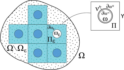
For fixed $\epsilon >0$, a two-phase medium associated to the disconnected domain $Q_{\epsilon }\cup {\omega }_{\epsilon }$ with the external boundary $\mathrm{\partial \Omega }$ and the interface $\mathrm{\partial }{\omega }_{\epsilon }$ is considered, see an example geometry in Figure 1.

Figure 1. A two-phase domain consisted of solid particles ${\omega }_{\epsilon }$ and the pore space $Q_{\epsilon }$ with the phase interface $\mathrm{\partial }{\omega }_{\epsilon }$.

Following [29,30] and based on the decomposition (1(1) $x=\epsilon ⌊\frac{x}{\epsilon }⌋+\epsilon \left\{\frac{x}{\epsilon }\right\}$(1) ), we introduce two linear continuous operators: the unfolding operator $f\left(x\right)\mapsto T_{\epsilon }:H^1\left(Q_{\epsilon }\right)\times H^1\left({\omega }_{\epsilon }\right)\mapsto L^2(\mathrm{\Omega };H^1(\mathrm{\Pi })\times H^1(\omega \left)\right)$, defined by (2) $\left(T_{\epsilon }f\right)(x,y)=\left\{\begin{array}{ll}f\left(\epsilon ⌊\frac{x}{\epsilon }⌋+\epsilon y\right),& \mathrm{a}.\mathrm{e}.\mathrm{for}x\in {\mathrm{\Omega }}_{\epsilon }\\ f\left(x\right),& \mathrm{a}.\mathrm{e}.\mathrm{for}x\in \mathrm{\Omega }\setminus {\mathrm{\Omega }}_{\epsilon }\end{array}\right.\mathrm{and}y\in \mathrm{\Pi }\cup \omega ,$(2) and its left-inverse operator $u(x,y)\mapsto T_{\epsilon }^{-1}:L^2(\mathrm{\Omega };H^1(\mathrm{\Pi })\times H^1(\omega \left)\right)\mapsto H^1\left(\bigcup _{l\in I^{\epsilon }}{\mathrm{\Pi }}_{\epsilon }^l\right)\times H^1\left({\omega }_{\epsilon }\right)\times H^1(\mathrm{\Omega }\setminus {\mathrm{\Omega }}_{\epsilon })$ called the averaging operator: (3) $\left(T_{\epsilon }^{-1}u\right)\left(x\right)=\left\{\begin{array}{ll}\frac{1}{|Y|}{\int }_{\mathrm{\Pi }\cup \omega }u\left(\epsilon ⌊\frac{x}{\epsilon }⌋+\epsilon z,\left\{\frac{x}{\epsilon }\right\}\right)\mathrm{d}z,& \mathrm{a}.\mathrm{e}.\mathrm{for}x\in {\mathrm{\Pi }}_{\epsilon }\cup {\omega }_{\epsilon },\\ \frac{1}{|Y|}{\int }_{\mathrm{\Pi }\cup \omega }u(x,y)\mathrm{d}y,& \mathrm{a}.\mathrm{e}.\mathrm{for}x\in \mathrm{\Omega }\setminus {\mathrm{\Omega }}_{\epsilon },\end{array}\right.$(3) where $|Y|$ stands for the Hausdorff measure of the set Y in ${\mathbb{R}}^d$. We note that $T_{\epsilon }^{-1}u$ in (3(3) $\left(T_{\epsilon }^{-1}u\right)\left(x\right)=\left\{\begin{array}{ll}\frac{1}{|Y|}{\int }_{\mathrm{\Pi }\cup \omega }u\left(\epsilon ⌊\frac{x}{\epsilon }⌋+\epsilon z,\left\{\frac{x}{\epsilon }\right\}\right)\mathrm{d}z,& \mathrm{a}.\mathrm{e}.\mathrm{for}x\in {\mathrm{\Pi }}_{\epsilon }\cup {\omega }_{\epsilon },\\ \frac{1}{|Y|}{\int }_{\mathrm{\Pi }\cup \omega }u(x,y)\mathrm{d}y,& \mathrm{a}.\mathrm{e}.\mathrm{for}x\in \mathrm{\Omega }\setminus {\mathrm{\Omega }}_{\epsilon },\end{array}\right.$(3) ) is discontinuous across $\mathrm{\partial }{Y}_{\epsilon }^l$ and $\mathrm{\partial }{\mathrm{\Omega }}_{\epsilon }$. In the homogenization theory, usually x refers to as a macro-variable, y as a micro-variable, and $(x,y)$ as the two-scale variables.

Lemma 2.1

Properties of the operators $T_{\epsilon }$ and $T_{\epsilon }^{-1}$ in the domain

For arbitrary functions $f,q,h\in H^1\left(Q_{\epsilon }\right)\times H^1\left({\omega }_{\epsilon }\right),$ the following properties hold: (4a) $\begin{array}{rl}& \left(\mathrm{i}\right)\text{invertibility:}\left(T_{\epsilon }^{-1}{T}_{\epsilon }\right)f\left(x\right)=f\left(x\right);\end{array}$(4a) (4b) $\begin{array}{rl}& \left(T_{\epsilon }{T}_{\epsilon }^{-1}u\right)(x,y)=u\left(y\right)\text{when }u\text{ is constant for }x\in Q_{\epsilon }\cup {\omega }_{\epsilon },\\ & \text{or a periodic function }u\left(y\right)\text{ of }y\in \mathrm{\Pi }\cup \omega \text{ for }x\in {\mathrm{\Pi }}_{\epsilon }\cup {\omega }_{\epsilon };\\ \left(\mathrm{ii}\right)& \text{product rule:}{T}_{\epsilon }\left(fq\right)=\left(T_{\epsilon }f\right)\left(T_{\epsilon }q\right);\end{array}$(4b) (4c) $\begin{array}{rl}\left(\mathrm{iii}\right)& \text{integration rules in the periodic domain and in the boundary layer:}\\ & {\int }_{{\mathrm{\Pi }}_{\epsilon }\cup {\omega }_{\epsilon }}f\left(x\right)q\left(x\right)\mathrm{d}x=\frac{1}{|Y|}{\int }_{{\mathrm{\Omega }}_{\epsilon }}{\int }_{\mathrm{\Pi }\cup \omega }\left(T_{\epsilon }f\right)(x,y)\cdot \left(T_{\epsilon }q\right)(x,y)\mathrm{d}y\mathrm{d}x,\end{array}$(4c) (4d) $\begin{array}{rl}& {\int }_{\mathrm{\Omega }\setminus {\mathrm{\Omega }}_{\epsilon }}f\left(x\right)q\left(x\right)\mathrm{d}x=\frac{1}{|Y|}{\int }_{\mathrm{\Omega }\setminus {\mathrm{\Omega }}_{\epsilon }}{\int }_{\mathrm{\Pi }\cup \omega }\left(T_{\epsilon }f\right)(x,y)\cdot \left(T_{\epsilon }q\right)(x,y)\mathrm{d}y\mathrm{d}x;\end{array}$(4d) (4e) $\begin{array}{rl}\left(\mathrm{iv}\right)& \text{boundedness of }{T}_{\epsilon }\text{ in the }{L}^2\text{-norm and the }{H}^1\text{-semi-norm:}\\ & {\int }_{Q_{\epsilon }\cup {\omega }_{\epsilon }}{h}^2\left(x\right)\mathrm{d}x=\frac{1}{|Y|}{\int }_{\mathrm{\Omega }}{\int }_{\mathrm{\Pi }\cup \omega }\left(T_{\epsilon }h{)}^2\right(x,y)\mathrm{d}y\mathrm{d}x,\end{array}$(4e) (4f) $\begin{array}{rl}& {\int }_{Q_{\epsilon }\cup {\omega }_{\epsilon }}|\mathrm{\nabla }h{|}^2\left(x\right)\mathrm{d}x=\frac{1}{{\epsilon }^2|Y|}{\int }_{\mathrm{\Omega }}{\int }_{\mathrm{\Pi }\cup \omega }|{\mathrm{\nabla }}_y\left(T_{\epsilon }h\right){|}^2(x,y)\mathrm{d}y\mathrm{d}x.\end{array}$(4f)

Proof.

(i) For $x\in \mathrm{\Omega }\setminus {\mathrm{\Omega }}_{\epsilon }$ and $f\in L^2(\mathrm{\Omega }\setminus {\mathrm{\Omega }}_{\epsilon })$, we calculate straightforwardly $\left(T_{\epsilon }^{-1}{T}_{\epsilon }\right)f\left(x\right)=\left(T_{\epsilon }^{-1}\right(T_{\epsilon }f\left)\right)\left(x\right)=\left(T_{\epsilon }^{-1}f\right)\left(x\right)=f\left(x\right)$. For $x\in {\mathrm{\Pi }}_{\epsilon }\cup {\omega }_{\epsilon }$ and $f\in L^2\left({\mathrm{\Pi }}_{\epsilon }\right)\times L^2\left({\omega }_{\epsilon }\right)$ according to (1(1) $x=\epsilon ⌊\frac{x}{\epsilon }⌋+\epsilon \left\{\frac{x}{\epsilon }\right\}$(1) ), the definitions (2(2) $\left(T_{\epsilon }f\right)(x,y)=\left\{\begin{array}{ll}f\left(\epsilon ⌊\frac{x}{\epsilon }⌋+\epsilon y\right),& \mathrm{a}.\mathrm{e}.\mathrm{for}x\in {\mathrm{\Omega }}_{\epsilon }\\ f\left(x\right),& \mathrm{a}.\mathrm{e}.\mathrm{for}x\in \mathrm{\Omega }\setminus {\mathrm{\Omega }}_{\epsilon }\end{array}\right.\mathrm{and}y\in \mathrm{\Pi }\cup \omega ,$(2) ) and (3(3) $\left(T_{\epsilon }^{-1}u\right)\left(x\right)=\left\{\begin{array}{ll}\frac{1}{|Y|}{\int }_{\mathrm{\Pi }\cup \omega }u\left(\epsilon ⌊\frac{x}{\epsilon }⌋+\epsilon z,\left\{\frac{x}{\epsilon }\right\}\right)\mathrm{d}z,& \mathrm{a}.\mathrm{e}.\mathrm{for}x\in {\mathrm{\Pi }}_{\epsilon }\cup {\omega }_{\epsilon },\\ \frac{1}{|Y|}{\int }_{\mathrm{\Pi }\cup \omega }u(x,y)\mathrm{d}y,& \mathrm{a}.\mathrm{e}.\mathrm{for}x\in \mathrm{\Omega }\setminus {\mathrm{\Omega }}_{\epsilon },\end{array}\right.$(3) ) with $z\in Y$ we have $\begin{array}{rl}\left(T_{\epsilon }^{-1}\right(T_{\epsilon }f\left)\right)\left(x\right)& =\frac{1}{|Y|}{\int }_{\mathrm{\Pi }\cup \omega }f\left(\epsilon ⌊\frac{\epsilon ⌊\frac{x}{\epsilon }⌋+\epsilon z}{\epsilon }⌋+\epsilon \left\{\frac{x}{\epsilon }\right\}\right)\mathrm{d}z\\ & =\frac{1}{|Y|}{\int }_{\mathrm{\Pi }\cup \omega }f\left(x\right)\mathrm{d}z=f\left(x\right),\end{array}$ since $\lfloor \lfloor x/\epsilon \rfloor +z\rfloor =\lfloor x/\epsilon \rfloor$, hence (4a(4a) $\begin{array}{rl}& \left(\mathrm{i}\right)\text{invertibility:}\left(T_{\epsilon }^{-1}{T}_{\epsilon }\right)f\left(x\right)=f\left(x\right);\end{array}$(4a) ) holds. The assertion for $T_{\epsilon }{T}_{\epsilon }^{-1}$ can be checked.

(ii) The identity (4b(4b) $\begin{array}{rl}& \left(T_{\epsilon }{T}_{\epsilon }^{-1}u\right)(x,y)=u\left(y\right)\text{when }u\text{ is constant for }x\in Q_{\epsilon }\cup {\omega }_{\epsilon },\\ & \text{or a periodic function }u\left(y\right)\text{ of }y\in \mathrm{\Pi }\cup \omega \text{ for }x\in {\mathrm{\Pi }}_{\epsilon }\cup {\omega }_{\epsilon };\\ \left(\mathrm{ii}\right)& \text{product rule:}{T}_{\epsilon }\left(fq\right)=\left(T_{\epsilon }f\right)\left(T_{\epsilon }q\right);\end{array}$(4b) ) is obvious.

(iii) The proof of (4c(4c) $\begin{array}{rl}\left(\mathrm{iii}\right)& \text{integration rules in the periodic domain and in the boundary layer:}\\ & {\int }_{{\mathrm{\Pi }}_{\epsilon }\cup {\omega }_{\epsilon }}f\left(x\right)q\left(x\right)\mathrm{d}x=\frac{1}{|Y|}{\int }_{{\mathrm{\Omega }}_{\epsilon }}{\int }_{\mathrm{\Pi }\cup \omega }\left(T_{\epsilon }f\right)(x,y)\cdot \left(T_{\epsilon }q\right)(x,y)\mathrm{d}y\mathrm{d}x,\end{array}$(4c) ) is known (see [29, Section 2]). In the boundary layer, we derive straightforwardly (4d(4d) $\begin{array}{rl}& {\int }_{\mathrm{\Omega }\setminus {\mathrm{\Omega }}_{\epsilon }}f\left(x\right)q\left(x\right)\mathrm{d}x=\frac{1}{|Y|}{\int }_{\mathrm{\Omega }\setminus {\mathrm{\Omega }}_{\epsilon }}{\int }_{\mathrm{\Pi }\cup \omega }\left(T_{\epsilon }f\right)(x,y)\cdot \left(T_{\epsilon }q\right)(x,y)\mathrm{d}y\mathrm{d}x;\end{array}$(4d) ) from (2(2) $\left(T_{\epsilon }f\right)(x,y)=\left\{\begin{array}{ll}f\left(\epsilon ⌊\frac{x}{\epsilon }⌋+\epsilon y\right),& \mathrm{a}.\mathrm{e}.\mathrm{for}x\in {\mathrm{\Omega }}_{\epsilon }\\ f\left(x\right),& \mathrm{a}.\mathrm{e}.\mathrm{for}x\in \mathrm{\Omega }\setminus {\mathrm{\Omega }}_{\epsilon }\end{array}\right.\mathrm{and}y\in \mathrm{\Pi }\cup \omega ,$(2) ) and (3(3) $\left(T_{\epsilon }^{-1}u\right)\left(x\right)=\left\{\begin{array}{ll}\frac{1}{|Y|}{\int }_{\mathrm{\Pi }\cup \omega }u\left(\epsilon ⌊\frac{x}{\epsilon }⌋+\epsilon z,\left\{\frac{x}{\epsilon }\right\}\right)\mathrm{d}z,& \mathrm{a}.\mathrm{e}.\mathrm{for}x\in {\mathrm{\Pi }}_{\epsilon }\cup {\omega }_{\epsilon },\\ \frac{1}{|Y|}{\int }_{\mathrm{\Pi }\cup \omega }u(x,y)\mathrm{d}y,& \mathrm{a}.\mathrm{e}.\mathrm{for}x\in \mathrm{\Omega }\setminus {\mathrm{\Omega }}_{\epsilon },\end{array}\right.$(3) ).

(iv) Taking first q=f=h, then $q=f=\mathrm{\nabla }h$ in (4c(4c) $\begin{array}{rl}\left(\mathrm{iii}\right)& \text{integration rules in the periodic domain and in the boundary layer:}\\ & {\int }_{{\mathrm{\Pi }}_{\epsilon }\cup {\omega }_{\epsilon }}f\left(x\right)q\left(x\right)\mathrm{d}x=\frac{1}{|Y|}{\int }_{{\mathrm{\Omega }}_{\epsilon }}{\int }_{\mathrm{\Pi }\cup \omega }\left(T_{\epsilon }f\right)(x,y)\cdot \left(T_{\epsilon }q\right)(x,y)\mathrm{d}y\mathrm{d}x,\end{array}$(4c) ) and (4d(4d) $\begin{array}{rl}& {\int }_{\mathrm{\Omega }\setminus {\mathrm{\Omega }}_{\epsilon }}f\left(x\right)q\left(x\right)\mathrm{d}x=\frac{1}{|Y|}{\int }_{\mathrm{\Omega }\setminus {\mathrm{\Omega }}_{\epsilon }}{\int }_{\mathrm{\Pi }\cup \omega }\left(T_{\epsilon }f\right)(x,y)\cdot \left(T_{\epsilon }q\right)(x,y)\mathrm{d}y\mathrm{d}x;\end{array}$(4d) ), summing them, and using $T_{\epsilon }\left(\mathrm{\nabla }f\right)=\left(1/\epsilon \right){\mathrm{\nabla }}_y\left(T_{\epsilon }f\right)$ due to the chain rule $\mathrm{\nabla }=\left(1/\epsilon \right){\mathrm{\nabla }}_y$, we arrive at (4e(4e) $\begin{array}{rl}\left(\mathrm{iv}\right)& \text{boundedness of }{T}_{\epsilon }\text{ in the }{L}^2\text{-norm and the }{H}^1\text{-semi-norm:}\\ & {\int }_{Q_{\epsilon }\cup {\omega }_{\epsilon }}{h}^2\left(x\right)\mathrm{d}x=\frac{1}{|Y|}{\int }_{\mathrm{\Omega }}{\int }_{\mathrm{\Pi }\cup \omega }\left(T_{\epsilon }h{)}^2\right(x,y)\mathrm{d}y\mathrm{d}x,\end{array}$(4e) ) and (4f(4f) $\begin{array}{rl}& {\int }_{Q_{\epsilon }\cup {\omega }_{\epsilon }}|\mathrm{\nabla }h{|}^2\left(x\right)\mathrm{d}x=\frac{1}{{\epsilon }^2|Y|}{\int }_{\mathrm{\Omega }}{\int }_{\mathrm{\Pi }\cup \omega }|{\mathrm{\nabla }}_y\left(T_{\epsilon }h\right){|}^2(x,y)\mathrm{d}y\mathrm{d}x.\end{array}$(4f) ). This completes the proof.

A function $f\in H^1\left(Q_{\epsilon }\right)\times H^1\left({\omega }_{\epsilon }\right)$ given in the two-phase domain allows discontinuity across the interface $\mathrm{\partial }{\omega }_{\epsilon }$, see zoom in Figure 1. In each local cell $Y_{\epsilon }^l$ we distinguish the negative face $(\mathrm{\partial }{\omega }_{\epsilon }^l{)}^{-}$ as the boundary of the particle ${\omega }_{\epsilon }^l$, and the positive face $(\mathrm{\partial }{\omega }_{\epsilon }^l{)}^{+}$ as the opposite part of the boundary of the pore ${\mathrm{\Pi }}_{\epsilon }^l$. Gathering over all local cells establishes the positive and negative faces of the interface as $\mathrm{\partial }{\omega }_{\epsilon }^{\pm }=\bigcup _{l\in I^{\epsilon }}(\mathrm{\partial }{\omega }_{\epsilon }^l{)}^{\pm }$. We set the interface jump of f across $\mathrm{\partial }{\omega }_{\epsilon }$ by (5) $\left[\right[f\left]\right]:=f{|}_{\mathrm{\partial }{\omega }_{\epsilon }^{+}}-f{|}_{\mathrm{\partial }{\omega }_{\epsilon }^{-}},$(5) where the corresponding traces of f at $\mathrm{\partial }{\omega }_{\epsilon }^{\pm }$ are well defined, see [31, Section 1.4]. Analogously, we define the interface jump for a function $u\left(y\right)\in H^1\left(\mathrm{\Pi }\right)\times H^1\left(\omega \right)$ in the unit cell as $\left[\right[u]{]}_y:=u{|}_{\mathrm{\partial }{\omega }^{+}}-u{|}_{\mathrm{\partial }{\omega }^{-}}$.

Motivated by the traces, we extend to the interface $\mathrm{\partial }{\omega }_{\epsilon }$ the unfolding operator $f\left(x\right)\mapsto T_{\epsilon }:L^2\left(\mathrm{\partial }{\omega }_{\epsilon }\right)\mapsto L^2\left({\mathrm{\Omega }}_{\epsilon }\right)\times L^2\left(\mathrm{\partial }\omega \right)$ by (6) $\left(T_{\epsilon }f\right)(x,y)=f\left(\epsilon ⌊\frac{x}{\epsilon }⌋+\epsilon y\right),\text{a.e. for }x\in {\mathrm{\Omega }}_{\epsilon }\text{and}y\in \mathrm{\partial }\omega ,$(6) and similarly the averaging operator $u(x,y)\mapsto T_{\epsilon }^{-1}:L^2\left({\mathrm{\Omega }}_{\epsilon }\right)\times L^2\left(\mathrm{\partial }\omega \right)\mapsto L^2\left(\mathrm{\partial }{\omega }_{\epsilon }\right)$, (7) $\left(T_{\epsilon }^{-1}u\right)\left(x\right)=\frac{1}{|Y|}{\int }_{\mathrm{\Pi }\cup \omega }u\left(\epsilon ⌊\frac{x}{\epsilon }⌋+\epsilon z,\left\{\frac{x}{\epsilon }\right\}\right)\mathrm{d}z,\text{a.e. for }x\in {\mathrm{\Omega }}_{\epsilon }.$(7) Their properties are stated below in the manner of Lemma 2.1.

Lemma 2.2

Properties of the operators $T_{\epsilon }$ and $T_{\epsilon }^{-1}$ at the interface

For arbitrary functions $f,q\in L^2\left(\mathrm{\partial }{\omega }_{\epsilon }\right),$ the following properties hold: (8a) $\begin{array}{rl}& \left(\mathrm{i}\right)\text{invertibility: }\left(T_{\epsilon }^{-1}{T}_{\epsilon }\right)f=f;\end{array}$(8a) (8b) $\begin{array}{rl}& \left(\mathrm{ii}\right)\text{product rule:}{T}_{\epsilon }\left(fq\right)=\left(T_{\epsilon }f\right)\left(T_{\epsilon }q\right);\end{array}$(8b) (8c) $\begin{array}{rl}& \left(\mathrm{iii}\right)\text{integration rule:}\\ & {\int }_{\mathrm{\partial }{\omega }_{\epsilon }}f\left(x\right)q\left(x\right)\mathrm{d}{S}_x=\frac{1}{\epsilon |Y|}{\int }_{{\mathrm{\Omega }}_{\epsilon }}{\int }_{\mathrm{\partial }\omega }\left(T_{\epsilon }f\right)(x,y)\cdot \left(T_{\epsilon }q\right)(x,y)\mathrm{d}{S}_y\mathrm{d}x;\end{array}$(8c) (8d) $\begin{array}{rl}& \left(\mathrm{iv}\right)\text{boundedness of }{T}_{\epsilon }\text{ in the }{L}^2\text{-norm:}\\ & {\int }_{\mathrm{\partial }{\omega }_{\epsilon }}{f}^2\left(x\right)\mathrm{d}{S}_x=\frac{1}{\epsilon |Y|}{\int }_{{\mathrm{\Omega }}_{\epsilon }}{\int }_{\mathrm{\partial }\omega }\left(T_{\epsilon }f{)}^2\right(x,y)\mathrm{d}{S}_y\mathrm{d}x.\end{array}$(8d)

Proof.

The proof of assertions (i) and (ii) is similar to the proof in Lemma 2.1. The proof of (8c(8c) $\begin{array}{rl}& \left(\mathrm{iii}\right)\text{integration rule:}\\ & {\int }_{\mathrm{\partial }{\omega }_{\epsilon }}f\left(x\right)q\left(x\right)\mathrm{d}{S}_x=\frac{1}{\epsilon |Y|}{\int }_{{\mathrm{\Omega }}_{\epsilon }}{\int }_{\mathrm{\partial }\omega }\left(T_{\epsilon }f\right)(x,y)\cdot \left(T_{\epsilon }q\right)(x,y)\mathrm{d}{S}_y\mathrm{d}x;\end{array}$(8c) ) is known (see [29, Section 4]). Taking q=f in (8c(8c) $\begin{array}{rl}& \left(\mathrm{iii}\right)\text{integration rule:}\\ & {\int }_{\mathrm{\partial }{\omega }_{\epsilon }}f\left(x\right)q\left(x\right)\mathrm{d}{S}_x=\frac{1}{\epsilon |Y|}{\int }_{{\mathrm{\Omega }}_{\epsilon }}{\int }_{\mathrm{\partial }\omega }\left(T_{\epsilon }f\right)(x,y)\cdot \left(T_{\epsilon }q\right)(x,y)\mathrm{d}{S}_y\mathrm{d}x;\end{array}$(8c) ) immediately follows formula (8d(8d) $\begin{array}{rl}& \left(\mathrm{iv}\right)\text{boundedness of }{T}_{\epsilon }\text{ in the }{L}^2\text{-norm:}\\ & {\int }_{\mathrm{\partial }{\omega }_{\epsilon }}{f}^2\left(x\right)\mathrm{d}{S}_x=\frac{1}{\epsilon |Y|}{\int }_{{\mathrm{\Omega }}_{\epsilon }}{\int }_{\mathrm{\partial }\omega }\left(T_{\epsilon }f{)}^2\right(x,y)\mathrm{d}{S}_y\mathrm{d}x.\end{array}$(8d) ) in (iv).

The geometric construction of the operators $T_{\epsilon }$ and $T_{\epsilon }^{-1}$ in this section will be used further for homogenization over $Q_{\epsilon }\cup {\omega }_{\epsilon }$ and $\mathrm{\partial }{\omega }_{\epsilon }$ as $\epsilon \searrow 0^{+}$.

3. Problem formulation

We formulate a generalized Poisson–Nernst–Planck system depending on a fixed parameter $\epsilon >0$, see [9–11]. We consider the number n of charged species with specific charges $z_i$, molar masses $m_i>0$, volume factors ${\beta }_i>0$, and unknown concentrations $c_i^{\epsilon }$ for $i=1,\dots ,n$ and $n⩾2$. By ${\varphi }^{\epsilon }$ we denote the overall electrostatic potential. The two-phase medium introduced in Section 2 will be characterized below separately in the pore phase $Q_{\epsilon }$ and the solid phase ${\omega }_{\epsilon }$.

For the time-space variables $(t,x)$ in $(0,\tau )\times (Q_{\epsilon }\cup {\omega }_{\epsilon })$ with a fixed final time $\tau >0$, we consider the following governing equations for species $i=1,\dots ,n$: (9a) $\begin{array}{rl}& \text{The Fick's law of diffusion:}\frac{\mathrm{\partial }{c}_i^{\epsilon }}{\mathrm{\partial }t}-\text{div}{J}_i^{\epsilon }=0;\end{array}$(9a) (9b) $\begin{array}{rl}& \text{cross-diffusion fluxes:}(J_i^{\epsilon }{)}^{\mathrm{\top }}=\sum _{j=1}^n{c}_j^{\epsilon }(\mathrm{\nabla }{\mu }_j^{\epsilon }+{\mathbf{1}}_{Q_{\epsilon }}\frac{{\epsilon }^{\kappa }\eta }{N_{A}C}{v}^{\epsilon }{)}^{\mathrm{\top }}{m}_i\left(T_{\epsilon }^{-1}{D}^{ij}\right);\end{array}$(9b) (9c) $\begin{array}{rl}& \text{ electrochemical potentials:}{\mu }_i^{\epsilon }=k_{\mathrm{B}}\mathrm{\Theta }\text{ln}\left({\beta }_i{c}_i^{\epsilon }\right)+{\mathbf{1}}_{Q_{\epsilon }}\frac{{\epsilon }^{\kappa }}{N_A}\left(\frac{1}{C}{p}^{\epsilon }+z_i{\varphi }^{\epsilon }\right);\end{array}$(9c) (9d) $\begin{array}{rl}& \text{the Darcy flow in pores:}\eta v^{\epsilon }+\mathrm{\nabla }{p}^{\epsilon }=-\left(\sum _{j=1}^n{z}_j{c}_j^{\epsilon }\right)\mathrm{\nabla }{\varphi }^{\epsilon },\text{div }{v}^{\epsilon }=0;\end{array}$(9d) (9e) $\begin{array}{rl}& \text{and the Gauss's flux law:}-\text{div}\left(\right(\mathrm{\nabla }{\varphi }^{\epsilon }{)}^{\mathrm{\top }}\left(T_{\epsilon }^{-1}A\right))={\mathbf{1}}_{Q_{\epsilon }}\sum _{j=1}^n{z}_j{c}_j^{\epsilon }.\end{array}$(9e) The indicator function ${\mathbf{1}}_{Q_{\epsilon }}$ is equal to 1 in $Q_{\epsilon }$, and 0 in ${\omega }_{\epsilon }$. The Equation (9c(9c) $\begin{array}{rl}& \text{ electrochemical potentials:}{\mu }_i^{\epsilon }=k_{\mathrm{B}}\mathrm{\Theta }\text{ln}\left({\beta }_i{c}_i^{\epsilon }\right)+{\mathbf{1}}_{Q_{\epsilon }}\frac{{\epsilon }^{\kappa }}{N_A}\left(\frac{1}{C}{p}^{\epsilon }+z_i{\varphi }^{\epsilon }\right);\end{array}$(9c) ) contains the Boltzmann constant $k_{\mathrm{B}}$, the temperature Θ, the Avogadro constant $N_A$, and $\kappa ⩾1$ in (9c(9c) $\begin{array}{rl}& \text{ electrochemical potentials:}{\mu }_i^{\epsilon }=k_{\mathrm{B}}\mathrm{\Theta }\text{ln}\left({\beta }_i{c}_i^{\epsilon }\right)+{\mathbf{1}}_{Q_{\epsilon }}\frac{{\epsilon }^{\kappa }}{N_A}\left(\frac{1}{C}{p}^{\epsilon }+z_i{\varphi }^{\epsilon }\right);\end{array}$(9c) ) allows us to average the non-linear diffusion fluxes (see (71(71) $\begin{array}{rl}& {\int }_0^{\tau }{\int }_{Q_{\epsilon }\cup {\omega }_{\epsilon }}\left\{\frac{\mathrm{\partial }{c}_i^{\epsilon }}{\mathrm{\partial }t}{\overline{c}}_i+k_{\mathrm{B}}\mathrm{\Theta }\left(\mathrm{\nabla }{c}_i^{\epsilon }{)}^{\mathrm{\top }}\right(T_{\epsilon }^{-1}D)\mathrm{\nabla }{\overline{c}}_i\right\}\mathrm{d}x\mathrm{d}t\\ & ={\int }_0^{\tau }{\int }_{\mathrm{\partial }{\omega }_{\epsilon }}{\epsilon }^2{g}_i({\hat{\mathit{c}}}^{\epsilon },{\hat{\varphi }}^{\epsilon })\left[\right[{\overline{c}}_i\left]\right]\mathrm{d}{S}_x\mathrm{d}t+O\left(\epsilon \right).\end{array}$(71) )). The fluxes contain the flow velocity following e.g. [3,4], and the dependence of potentials on the fluid pressure is due to the works by Dreyer (see [1,2]). The Equations (9b(9b) $\begin{array}{rl}& \text{cross-diffusion fluxes:}(J_i^{\epsilon }{)}^{\mathrm{\top }}=\sum _{j=1}^n{c}_j^{\epsilon }(\mathrm{\nabla }{\mu }_j^{\epsilon }+{\mathbf{1}}_{Q_{\epsilon }}\frac{{\epsilon }^{\kappa }\eta }{N_{A}C}{v}^{\epsilon }{)}^{\mathrm{\top }}{m}_i\left(T_{\epsilon }^{-1}{D}^{ij}\right);\end{array}$(9b) )–(9d(9d) $\begin{array}{rl}& \text{the Darcy flow in pores:}\eta v^{\epsilon }+\mathrm{\nabla }{p}^{\epsilon }=-\left(\sum _{j=1}^n{z}_j{c}_j^{\epsilon }\right)\mathrm{\nabla }{\varphi }^{\epsilon },\text{div }{v}^{\epsilon }=0;\end{array}$(9d) ) will be not solved with respect to electro-chemical potentials $({\mu }_1^{\epsilon },\dots ,{\mu }_n^{\epsilon })$, flow velocity vector $v^{\epsilon }=(v_1^{\epsilon },\dots ,v_d^{\epsilon })$ with the drug coefficient η, and the pressure $p^{\epsilon }$, but rather reduced within a weak formulation (see (22(22a) $\begin{array}{rl}& {\int }_0^{\tau }{\int }_{Q_{\epsilon }\cup {\omega }_{\epsilon }}\left\{\frac{\mathrm{\partial }{c}_i^{\epsilon }}{\mathrm{\partial }t}{\overline{c}}_i+\sum _{j=1}^n{\left[k_{\mathrm{B}}\mathrm{\Theta \nabla }{c}_j^{\epsilon }+{\epsilon }^{\kappa }{\mathbf{1}}_{Q_{\epsilon }}{\mathrm{{\rm Y}}}_j\left({\mathit{c}}^{\epsilon }\right)\mathrm{\nabla }{\varphi }^{\epsilon }\right]}^{\mathrm{\top }}{m}_i\left(T_{\epsilon }^{-1}{D}^{ij}\right)\mathrm{\nabla }{\overline{c}}_i\right\}\mathrm{d}x\mathrm{d}t\\ & ={\int }_0^{\tau }{\int }_{\mathrm{\partial }{\omega }_{\epsilon }}{\epsilon }^2{g}_i({\hat{\mathit{c}}}^{\epsilon },{\hat{\varphi }}^{\epsilon })\left[\right[{\overline{c}}_i\left]\right]\mathrm{d}{S}_x\mathrm{d}t,i=1,\dots ,n,\end{array}$(22a) )). Conversely, after finding $(c_1^{\epsilon },\dots ,c_n^{\epsilon })$ and ${\varphi }^{\epsilon }$, all the entropy variables $({\mu }_1^{\epsilon },\dots ,{\mu }_n^{\epsilon })$, $v^{\epsilon }$, $p^{\epsilon }$ can be restored from the Equations (9c(9c) $\begin{array}{rl}& \text{ electrochemical potentials:}{\mu }_i^{\epsilon }=k_{\mathrm{B}}\mathrm{\Theta }\text{ln}\left({\beta }_i{c}_i^{\epsilon }\right)+{\mathbf{1}}_{Q_{\epsilon }}\frac{{\epsilon }^{\kappa }}{N_A}\left(\frac{1}{C}{p}^{\epsilon }+z_i{\varphi }^{\epsilon }\right);\end{array}$(9c) ) and (9d(9d) $\begin{array}{rl}& \text{the Darcy flow in pores:}\eta v^{\epsilon }+\mathrm{\nabla }{p}^{\epsilon }=-\left(\sum _{j=1}^n{z}_j{c}_j^{\epsilon }\right)\mathrm{\nabla }{\varphi }^{\epsilon },\text{div }{v}^{\epsilon }=0;\end{array}$(9d) ) supported by suitable boundary conditions.

In (9e(9e) $\begin{array}{rl}& \text{and the Gauss's flux law:}-\text{div}\left(\right(\mathrm{\nabla }{\varphi }^{\epsilon }{)}^{\mathrm{\top }}\left(T_{\epsilon }^{-1}A\right))={\mathbf{1}}_{Q_{\epsilon }}\sum _{j=1}^n{z}_j{c}_j^{\epsilon }.\end{array}$(9e) ) and (9b(9b) $\begin{array}{rl}& \text{cross-diffusion fluxes:}(J_i^{\epsilon }{)}^{\mathrm{\top }}=\sum _{j=1}^n{c}_j^{\epsilon }(\mathrm{\nabla }{\mu }_j^{\epsilon }+{\mathbf{1}}_{Q_{\epsilon }}\frac{{\epsilon }^{\kappa }\eta }{N_{A}C}{v}^{\epsilon }{)}^{\mathrm{\top }}{m}_i\left(T_{\epsilon }^{-1}{D}^{ij}\right);\end{array}$(9b) ) the d-by-d matrices A and $D^{ij}$ for $i,j=1,\dots ,n$ imply the electric permittivity and diffusivity, respectively. They can be discontinuous in the two-phase unit cell $\mathrm{\Pi }\cup \omega$ and satisfy the following assumptions.

• $A\left(y\right)\in {\mathbb{R}}^{d\times d}$ for $y\in \mathrm{\Pi }\cup \omega$ is uniformly bounded and symmetric positive definite (spd) matrix: (10) $\mathrm{there}\mathrm{exist}0<\underset{\_}{a}⩽\overline{a}\mathrm{such}\mathrm{that}\underset{\_}{a}|\xi {|}^2⩽{\xi }^{\mathrm{\top }}A\left(y\right)\xi ⩽\overline{a}|\xi {|}^2\text{for }\xi \in {\mathbb{R}}^d;$(10)

• $m_i{D}^{ij}\left(y\right)\in {\mathbb{R}}^{d\times d}$ for $y\in \mathrm{\Pi }\cup \omega$ are uniformly bounded and elliptic matrices: there exist $0<\underset{\_}{d}⩽\overline{d}$ such that $\underset{\_}{d}\sum _{i=1}^n|{\xi }_i{|}^2⩽\sum _{i,j=1}^n{\xi }_i^{\mathrm{\top }}{m}_i{D}^{ij}\left(y\right){\xi }_j⩽\overline{d}\sum _{i=1}^n|{\xi }_i{|}^2\text{for }{\xi }_1,\dots ,{\xi }_n\in {\mathbb{R}}^d;$

• the mass balance needs a symmetric positive definite (see (13(13) $\underset{\_}{d}|\xi {|}^2⩽{\xi }^{\mathrm{\top }}D\left(y\right)\xi ⩽\overline{d}|\xi {|}^2\text{for }\xi \in {\mathbb{R}}^d.$(13) ) below) matrix $\tilde{D}\left(y\right)\in {\mathbb{R}}^{d\times d}$ for $y\in \mathrm{\Pi }\cup \omega$ such that: (11) $\sum _{i=1}^n{m}_i{D}^{ij}\left(y\right)=\tilde{D}\left(y\right)\text{for }j=1,\dots ,n.$(11)

It is worth noting that conditions (11(11) $\sum _{i=1}^n{m}_i{D}^{ij}\left(y\right)=\tilde{D}\left(y\right)\text{for }j=1,\dots ,n.$(11) ) together with (14a(14a) $\begin{array}{rl}\mathrm{the}\mathrm{total}\mathrm{mass}\mathrm{balance}:& \sum _{i=1}^n{c}_i^{\epsilon }=C;\end{array}$(14a) ) below are sufficient to conserve the mass within the laws (9b(9b) $\begin{array}{rl}& \text{cross-diffusion fluxes:}(J_i^{\epsilon }{)}^{\mathrm{\top }}=\sum _{j=1}^n{c}_j^{\epsilon }(\mathrm{\nabla }{\mu }_j^{\epsilon }+{\mathbf{1}}_{Q_{\epsilon }}\frac{{\epsilon }^{\kappa }\eta }{N_{A}C}{v}^{\epsilon }{)}^{\mathrm{\top }}{m}_i\left(T_{\epsilon }^{-1}{D}^{ij}\right);\end{array}$(9b) )–(9d(9d) $\begin{array}{rl}& \text{the Darcy flow in pores:}\eta v^{\epsilon }+\mathrm{\nabla }{p}^{\epsilon }=-\left(\sum _{j=1}^n{z}_j{c}_j^{\epsilon }\right)\mathrm{\nabla }{\varphi }^{\epsilon },\text{div }{v}^{\epsilon }=0;\end{array}$(9d) ) as follows: $\begin{array}{rl}\sum _{i=1}^n(J_i^{\epsilon }{)}^{\mathrm{\top }}& =\sum _{j=1}^n{c}_j^{\epsilon }{\left(\mathrm{\nabla }{\mu }_j^{\epsilon }+{\mathbf{1}}_{Q_{\epsilon }}\frac{{\epsilon }^{\kappa }\eta }{N_{A}C}{v}^{\epsilon }\right)}^{\mathrm{\top }}{T}_{\epsilon }^{-1}\tilde{D}=\left\{k_{\mathrm{B}}\mathrm{\Theta }\sum _{j=1}^n\mathrm{\nabla }{c}_j^{\epsilon }\right.\\ & {\left.+{\mathbf{1}}_{Q_{\epsilon }}\frac{{\epsilon }^{\kappa }}{N_A}\left(\frac{1}{C}\left(\sum _{j=1}^n{c}_j^{\epsilon }\right)\mathrm{\nabla }{p}^{\epsilon }+\left(\sum _{j=1}^n{z}_j{c}_j^{\epsilon }\right)\mathrm{\nabla }{\varphi }^{\epsilon }+\frac{\eta }{C}\left(\sum _{j=1}^n{c}_j^{\epsilon }\right)v^{\epsilon }\right)\right\}}^{\mathrm{\top }}{T}_{\epsilon }^{-1}\tilde{D}=0.\end{array}$ For homogenization reason, we assume that the diffusivity matrices $D^{ij}$ from (11(11) $\sum _{i=1}^n{m}_i{D}^{ij}\left(y\right)=\tilde{D}\left(y\right)\text{for }j=1,\dots ,n.$(11) ) admit the asymptotic decomposition as follows (12) $m_i{D}^{ij}\left(y\right)={\delta }_{ij}D\left(y\right)+\epsilon {\tilde{D}}^{ij}\left(y\right)\text{for }y\in \mathrm{\Pi }\cup \omega ,$(12) with d-by-d matrices ${\tilde{D}}^{ij}$, $i,j=1,\dots ,n$ and a d-by-d uniformly bounded, symmetric positive definite matrix D such that (13) $\underset{\_}{d}|\xi {|}^2⩽{\xi }^{\mathrm{\top }}D\left(y\right)\xi ⩽\overline{d}|\xi {|}^2\text{for }\xi \in {\mathbb{R}}^d.$(13) The oscillating matrices $\left(T_{\epsilon }^{-1}{D}^{ij}\right)\left(x\right)=D^{ij}\left(\right\{x/\epsilon \left\}\right)$ and $\left(T_{\epsilon }^{-1}A\right)\left(x\right)=A\left(\right\{x/\epsilon \left\}\right)$ in the Equations (9b(9b) $\begin{array}{rl}& \text{cross-diffusion fluxes:}(J_i^{\epsilon }{)}^{\mathrm{\top }}=\sum _{j=1}^n{c}_j^{\epsilon }(\mathrm{\nabla }{\mu }_j^{\epsilon }+{\mathbf{1}}_{Q_{\epsilon }}\frac{{\epsilon }^{\kappa }\eta }{N_{A}C}{v}^{\epsilon }{)}^{\mathrm{\top }}{m}_i\left(T_{\epsilon }^{-1}{D}^{ij}\right);\end{array}$(9b) ) and (9e(9e) $\begin{array}{rl}& \text{and the Gauss's flux law:}-\text{div}\left(\right(\mathrm{\nabla }{\varphi }^{\epsilon }{)}^{\mathrm{\top }}\left(T_{\epsilon }^{-1}A\right))={\mathbf{1}}_{Q_{\epsilon }}\sum _{j=1}^n{z}_j{c}_j^{\epsilon }.\end{array}$(9e) ) are defined in Ω, and they are periodic in ${\mathrm{\Omega }}_{\epsilon }$.

A constant C>0 in (9c(9c) $\begin{array}{rl}& \text{ electrochemical potentials:}{\mu }_i^{\epsilon }=k_{\mathrm{B}}\mathrm{\Theta }\text{ln}\left({\beta }_i{c}_i^{\epsilon }\right)+{\mathbf{1}}_{Q_{\epsilon }}\frac{{\epsilon }^{\kappa }}{N_A}\left(\frac{1}{C}{p}^{\epsilon }+z_i{\varphi }^{\epsilon }\right);\end{array}$(9c) ) stands for the summary concentration. For the physical consistency, species concentrations need to satisfy in pores $(0,\tau )\times Q_{\epsilon }$: (14a) $\begin{array}{rl}\mathrm{the}\mathrm{total}\mathrm{mass}\mathrm{balance}:& \sum _{i=1}^n{c}_i^{\epsilon }=C;\end{array}$(14a) (14b) $\begin{array}{rl}\mathrm{the}\mathrm{positivity}:& c_i^{\epsilon }>0,\text{for }i=1,\dots ,n.\end{array}$(14b)

The system (9(9a) $\begin{array}{rl}& \text{The Fick's law of diffusion:}\frac{\mathrm{\partial }{c}_i^{\epsilon }}{\mathrm{\partial }t}-\text{div}{J}_i^{\epsilon }=0;\end{array}$(9a) ) is supported by the initial condition for $c_i^{\mathrm{in}}\in H^1\left(\mathrm{\Omega }\right)$: (15) $c_i^{\epsilon }=c_i^{\mathrm{in}}\text{on }{Q}_{\epsilon }\cup {\omega }_{\epsilon },$(15) where the initial data satisfy the relations in the manner of (14(14a) $\begin{array}{rl}\mathrm{the}\mathrm{total}\mathrm{mass}\mathrm{balance}:& \sum _{i=1}^n{c}_i^{\epsilon }=C;\end{array}$(14a) ) in pores $Q_{\epsilon }$: (16) $\sum _{i=1}^n{c}_i^{\mathrm{in}}=C,c_i^{\mathrm{in}}>0,\mathrm{for}i=1,\dots ,n.$(16) For given functions $c_i^{\mathrm{D}}\in H^1(0,\tau ;L^2(\mathrm{\Omega }\left)\right)\cap L^2(0,\tau ;H^1(\mathrm{\Omega }\left)\right)$ and ${\varphi }^{\mathrm{D}}\in L^{\mathrm{\infty }}(0,\tau ;H^1(\mathrm{\Omega }\left)\right)$ the Dirichlet boundary conditions are: (17) $c_i^{\epsilon }=c_i^{\mathrm{D}},\text{for }i=1,\dots ,n,{\varphi }^{\epsilon }={\varphi }^{\mathrm{D}}\text{on }(0,\tau )\times \mathrm{\partial \Omega },$(17) with the boundary data satisfying the similar relations and compatibility: (18) $\sum _{i=1}^n{c}_i^{\mathrm{D}}=C,c_i^{\mathrm{D}}>0\text{on }(0,\tau )\times \mathrm{\partial \Omega };c_i^{\mathrm{D}}(0,\cdot )=c_i^{\mathrm{in}}\text{in }{Q}_{\epsilon }\cup {\omega }_{\epsilon }.$(18) The most delicate part of modelling is the interface conditions on $(0,\tau )\times \mathrm{\partial }{\omega }_{\epsilon }$: (19a) $\begin{array}{rl}& \left[\right[J_i^{\epsilon }\left]\right]\nu =0,-J_i^{\epsilon }\nu ={\epsilon }^2{g}_i({\hat{\mathit{c}}}^{\epsilon },{\hat{\varphi }}^{\epsilon });\end{array}$(19a) (19b) $\begin{array}{rl}& \left[\right[\left(\mathrm{\nabla }{\varphi }^{\epsilon }{)}^{\mathrm{\top }}\right(T_{\epsilon }^{-1}A\left)\right]]\nu =0,-(\mathrm{\nabla }{\varphi }^{\epsilon }{)}^{\mathrm{\top }}\left(T_{\epsilon }^{-1}A\right)\nu +\frac{\alpha }{\epsilon }\left[\right[{\varphi }^{\epsilon }\left]\right]=T_{\epsilon }^{-1}g,\end{array}$(19b) where the jump across $\mathrm{\partial }{\omega }_{\epsilon }$ is defined in (5(5) $\left[\right[f\left]\right]:=f{|}_{\mathrm{\partial }{\omega }_{\epsilon }^{+}}-f{|}_{\mathrm{\partial }{\omega }_{\epsilon }^{-}},$(5) ). The notation ${\hat{\mathit{c}}}^{\epsilon }:=({\mathit{c}}^{\epsilon }{|}_{\mathrm{\partial }{\omega }_{\epsilon }^{+}},{\mathit{c}}^{\epsilon }{|}_{\mathrm{\partial }{\omega }_{\epsilon }^{-}})$ and ${\hat{\varphi }}^{\epsilon }:=({\varphi }^{\epsilon }{|}_{\mathrm{\partial }{\omega }_{\epsilon }^{+}},{\varphi }^{\epsilon }{|}_{\mathrm{\partial }{\omega }_{\epsilon }^{-}})$ implies the pair of traces at the phase interface $\mathrm{\partial }{\omega }_{\epsilon }$. The function $g\in L^{\mathrm{\infty }}(0,\tau ;L^2(\mathrm{\partial }\omega \left)\right)$ denotes the electric current through the interface in the unit cell, and $\left(T_{\epsilon }^{-1}g\right)\left(x\right)=g\left(\right\{x/\epsilon \left\}\right)$ in (19b(19b) $\begin{array}{rl}& \left[\right[\left(\mathrm{\nabla }{\varphi }^{\epsilon }{)}^{\mathrm{\top }}\right(T_{\epsilon }^{-1}A\left)\right]]\nu =0,-(\mathrm{\nabla }{\varphi }^{\epsilon }{)}^{\mathrm{\top }}\left(T_{\epsilon }^{-1}A\right)\nu +\frac{\alpha }{\epsilon }\left[\right[{\varphi }^{\epsilon }\left]\right]=T_{\epsilon }^{-1}g,\end{array}$(19b) ) is periodic at $\mathrm{\partial }{\omega }_{\epsilon }$. The capacitance density $\alpha >0$. The equality in (19b(19b) $\begin{array}{rl}& \left[\right[\left(\mathrm{\nabla }{\varphi }^{\epsilon }{)}^{\mathrm{\top }}\right(T_{\epsilon }^{-1}A\left)\right]]\nu =0,-(\mathrm{\nabla }{\varphi }^{\epsilon }{)}^{\mathrm{\top }}\left(T_{\epsilon }^{-1}A\right)\nu +\frac{\alpha }{\epsilon }\left[\right[{\varphi }^{\epsilon }\left]\right]=T_{\epsilon }^{-1}g,\end{array}$(19b) ) implies that the potential jump is asymptotically small $\left[\right[{\varphi }^{\epsilon }\left]\right]=O\left(\epsilon \right)$ in the electric double layer. The factor ${\epsilon }^2$ in (19a(19a) $\begin{array}{rl}& \left[\right[J_i^{\epsilon }\left]\right]\nu =0,-J_i^{\epsilon }\nu ={\epsilon }^2{g}_i({\hat{\mathit{c}}}^{\epsilon },{\hat{\varphi }}^{\epsilon });\end{array}$(19a) ) is used in Theorem 5.1 for averaging of the nonlinear, thus non-periodic interface data (see (72(72) $\begin{array}{rl}\left|{\int }_{\mathrm{\partial }{\omega }_{\epsilon }}{\epsilon }^2{g}_i({\hat{\mathit{c}}}^{\epsilon },{\hat{\varphi }}^{\epsilon })\left[\right[{\overline{c}}_i\left]\right]\mathrm{d}{S}_x\right|& ⩽{\epsilon }^2\left\{\frac{1}{4}{\int }_{\mathrm{\partial }{\omega }_{\epsilon }}|g_i({\hat{\mathit{c}}}^{\epsilon },{\hat{\varphi }}^{\epsilon }){|}^2\mathrm{d}{S}_x+{\int }_{\mathrm{\partial }{\omega }_{\epsilon }}|\left[\right[{\overline{c}}_i\left]\right]{|}^2\mathrm{d}{S}_x\right\}\\ & ⩽{\epsilon }^2\left\{\frac{K_{\mathrm{g}}}{4}|\mathrm{\partial }{\omega }_{\epsilon }|+\frac{K_0}{\epsilon }\parallel {\overline{c}}_i{\parallel }_{H^1\left(Q_{\epsilon }\right)\times H^1\left({\omega }_{\epsilon }\right)}^2\right\}=O\left(\epsilon \right).\end{array}$(72) )), and the factor $1/\epsilon$ in (19b(19b) $\begin{array}{rl}& \left[\right[\left(\mathrm{\nabla }{\varphi }^{\epsilon }{)}^{\mathrm{\top }}\right(T_{\epsilon }^{-1}A\left)\right]]\nu =0,-(\mathrm{\nabla }{\varphi }^{\epsilon }{)}^{\mathrm{\top }}\left(T_{\epsilon }^{-1}A\right)\nu +\frac{\alpha }{\epsilon }\left[\right[{\varphi }^{\epsilon }\left]\right]=T_{\epsilon }^{-1}g,\end{array}$(19b) ) will be explained later in (24(24) $\begin{array}{rl}\parallel f{\parallel }_{H^1\left(Q_{\epsilon }\right)\times H^1\left({\omega }_{\epsilon }\right)}^2& ={\int }_{Q_{\epsilon }\cup {\omega }_{\epsilon }}(f^2+|\mathrm{\nabla }f{|}^2)\mathrm{d}x\\ & ⩽k_{\mathrm{DP}}\left\{{\int }_{Q_{\epsilon }\cup {\omega }_{\epsilon }}|\mathrm{\nabla }f{|}^2\mathrm{d}x+\frac{1}{\epsilon }{\int }_{\mathrm{\partial }{\omega }_{\epsilon }}\left[\right[f]{]}^2\mathrm{d}{S}_x\right\}.\end{array}$(24) ). For modelling and numerical simulations of data for scaling of potentials, interface and boundary conditions, we refer to [25].

In (19a(19a) $\begin{array}{rl}& \left[\right[J_i^{\epsilon }\left]\right]\nu =0,-J_i^{\epsilon }\nu ={\epsilon }^2{g}_i({\hat{\mathit{c}}}^{\epsilon },{\hat{\varphi }}^{\epsilon });\end{array}$(19a) ), the functions $(\hat{\mathit{c}},\hat{\varphi })\mapsto g_i$, ${\mathbb{R}}^{2n}\times {\mathbb{R}}^2\mapsto \mathbb{R}$, $i=1,\dots ,n$, describing the boundary fluxes of species with respect to the traces $\hat{\mathit{c}}:=(\mathit{c}{|}_{\mathrm{\partial }{\omega }_{\epsilon }^{+}},\mathit{c}{|}_{\mathrm{\partial }{\omega }_{\epsilon }^{-}})$ and $\hat{\varphi }:=(\varphi {|}_{\mathrm{\partial }{\omega }_{\epsilon }^{+}},\varphi {|}_{\mathrm{\partial }{\omega }_{\epsilon }^{-}})$ of the variables $\mathit{c}=(c_1,\dots ,c_n)$ and ϕ, should satisfy (20a) $\begin{array}{rl}\mathrm{balance}\mathrm{of}\mathrm{the}\mathrm{mass}:& \sum _{i=1}^n{g}_i(\hat{\mathit{c}},\hat{\varphi })=0;\end{array}$(20a) (20b) $\begin{array}{rl}\mathrm{positive}\mathrm{production}\mathrm{rate}\mathrm{at}\mathrm{\partial }{\omega }_{\epsilon }^{+}:& g_i(\hat{\mathit{c}},\hat{\varphi })\cdot min(0,c_i{|}_{\mathrm{\partial }{\omega }_{\epsilon }^{+}})=0;\end{array}$(20b) (20c) $\begin{array}{rl}\mathrm{uniform}\mathrm{boundedness}(K_{\mathrm{g}}>0):& |g_i(\hat{\mathit{c}},\hat{\varphi }){|}^2⩽K_{\mathrm{g}}.\end{array}$(20c) The example of $g_i$ satisfying all assumptions (20(20a) $\begin{array}{rl}\mathrm{balance}\mathrm{of}\mathrm{the}\mathrm{mass}:& \sum _{i=1}^n{g}_i(\hat{\mathit{c}},\hat{\varphi })=0;\end{array}$(20a) ) can be found in [9,10], e.g. $g_1(\hat{\mathit{c}},\hat{\varphi })=\frac{max(0,c_1{|}_{\mathrm{\partial }{\omega }_{\epsilon }^{+}})max(0,c_2{|}_{\mathrm{\partial }{\omega }_{\epsilon }^{+}})}{[\sum _{k=1}^{n}max(0,c_k{|}_{\mathrm{\partial }{\omega }_{\epsilon }^{+}}){]}^2},g_2(\hat{\mathit{c}},\hat{\varphi })=-g_1(\hat{\mathit{c}},\hat{\varphi }),$ and $g_k(\hat{\mathit{c}},\hat{\varphi })=0\mathrm{for}k⩾3$.

A weak formulation of the generalized PNP problem is the following one: Find $(c_1^{\epsilon },\dots ,c_n^{\epsilon })$ and ${\varphi }^{\epsilon }$ such that for $i=1,\dots ,n$: (21a) $\begin{array}{rl}& c_i^{\epsilon }\in L^{\mathrm{\infty }}(0,\tau ;L^2(Q_{\epsilon })\times L^2({\omega }_{\epsilon }\left)\right)\cap L^2(0,\tau ;H^1(Q_{\epsilon })\times H^1({\omega }_{\epsilon }\left)\right),\end{array}$(21a) (21b) $\begin{array}{rl}& {\varphi }^{\epsilon }\in L^{\mathrm{\infty }}(0,\tau ;H^1(Q_{\epsilon })\times H^1({\omega }_{\epsilon }\left)\right),c_i^{\epsilon }\mathrm{\nabla }{\varphi }_i^{\epsilon }\in L^2\left(\right(0,\tau )\times (Q_{\epsilon }\cup {\omega }_{\epsilon }\left)\right),\end{array}$(21b) which satisfy the Dirichlet boundary conditions (17(17) $c_i^{\epsilon }=c_i^{\mathrm{D}},\text{for }i=1,\dots ,n,{\varphi }^{\epsilon }={\varphi }^{\mathrm{D}}\text{on }(0,\tau )\times \mathrm{\partial \Omega },$(17) ), the initial conditions (15(15) $c_i^{\epsilon }=c_i^{\mathrm{in}}\text{on }{Q}_{\epsilon }\cup {\omega }_{\epsilon },$(15) ), the total mass balance and positivity conditions (14(14a) $\begin{array}{rl}\mathrm{the}\mathrm{total}\mathrm{mass}\mathrm{balance}:& \sum _{i=1}^n{c}_i^{\epsilon }=C;\end{array}$(14a) ), and fulfil the equations: (22a) $\begin{array}{rl}& {\int }_0^{\tau }{\int }_{Q_{\epsilon }\cup {\omega }_{\epsilon }}\left\{\frac{\mathrm{\partial }{c}_i^{\epsilon }}{\mathrm{\partial }t}{\overline{c}}_i+\sum _{j=1}^n{\left[k_{\mathrm{B}}\mathrm{\Theta \nabla }{c}_j^{\epsilon }+{\epsilon }^{\kappa }{\mathbf{1}}_{Q_{\epsilon }}{\mathrm{{\rm Y}}}_j\left({\mathit{c}}^{\epsilon }\right)\mathrm{\nabla }{\varphi }^{\epsilon }\right]}^{\mathrm{\top }}{m}_i\left(T_{\epsilon }^{-1}{D}^{ij}\right)\mathrm{\nabla }{\overline{c}}_i\right\}\mathrm{d}x\mathrm{d}t\\ & ={\int }_0^{\tau }{\int }_{\mathrm{\partial }{\omega }_{\epsilon }}{\epsilon }^2{g}_i({\hat{\mathit{c}}}^{\epsilon },{\hat{\varphi }}^{\epsilon })\left[\right[{\overline{c}}_i\left]\right]\mathrm{d}{S}_x\mathrm{d}t,i=1,\dots ,n,\end{array}$(22a) (22b) $\begin{array}{rl}& {\int }_{Q_{\epsilon }\cup {\omega }_{\epsilon }}\left(\left(\mathrm{\nabla }{\varphi }^{\epsilon }{)}^{\mathrm{\top }}\right(T_{\epsilon }^{-1}A)\mathrm{\nabla }\overline{\varphi }-{\mathbf{1}}_{Q_{\epsilon }}\left(\sum _{k=1}^n{z}_k{c}_k^{\epsilon }\right)\overline{\varphi }\right)\mathrm{d}x+\frac{\alpha }{\epsilon }{\int }_{\mathrm{\partial }{\omega }_{\epsilon }}\left[\right[{\varphi }^{\epsilon }\left]\right]\left[\right[\overline{\varphi }\left]\right]\mathrm{d}{S}_x\\ & ={\int }_{\mathrm{\partial }{\omega }_{\epsilon }}\left(T_{\epsilon }^{-1}g\right)\left[\right[\overline{\varphi }\left]\right]\mathrm{d}{S}_x,t\in (0,\tau ),\end{array}$(22b) for all test functions ${\overline{c}}_i\in H^1(0,\tau ;L^2(Q_{\epsilon })\times L^2({\omega }_{\epsilon }\left)\right)\cap L^2(0,\tau ;H^1(Q_{\epsilon })\times H^1({\omega }_{\epsilon }\left)\right)$ and $\overline{\varphi }\in H^1\left(Q_{\epsilon }\right)\times H^1\left({\omega }_{\epsilon }\right)$ such that ${\overline{c}}_i=0$ on $(0,\tau )\times \mathrm{\partial \Omega }$ and $\overline{\varphi }=0$ on $\mathrm{\partial \Omega }$. In (22a(22a) $\begin{array}{rl}& {\int }_0^{\tau }{\int }_{Q_{\epsilon }\cup {\omega }_{\epsilon }}\left\{\frac{\mathrm{\partial }{c}_i^{\epsilon }}{\mathrm{\partial }t}{\overline{c}}_i+\sum _{j=1}^n{\left[k_{\mathrm{B}}\mathrm{\Theta \nabla }{c}_j^{\epsilon }+{\epsilon }^{\kappa }{\mathbf{1}}_{Q_{\epsilon }}{\mathrm{{\rm Y}}}_j\left({\mathit{c}}^{\epsilon }\right)\mathrm{\nabla }{\varphi }^{\epsilon }\right]}^{\mathrm{\top }}{m}_i\left(T_{\epsilon }^{-1}{D}^{ij}\right)\mathrm{\nabla }{\overline{c}}_i\right\}\mathrm{d}x\mathrm{d}t\\ & ={\int }_0^{\tau }{\int }_{\mathrm{\partial }{\omega }_{\epsilon }}{\epsilon }^2{g}_i({\hat{\mathit{c}}}^{\epsilon },{\hat{\varphi }}^{\epsilon })\left[\right[{\overline{c}}_i\left]\right]\mathrm{d}{S}_x\mathrm{d}t,i=1,\dots ,n,\end{array}$(22a) ) the following notation was used for short: (23) ${\mathrm{{\rm Y}}}_j\left(\mathit{c}\right):=\frac{c_j}{N_A}\left(z_j-\frac{1}{C}\sum _{k=1}^n{z}_k{c}_k\right).$(23) The time-derivative in (22a(22a) $\begin{array}{rl}& {\int }_0^{\tau }{\int }_{Q_{\epsilon }\cup {\omega }_{\epsilon }}\left\{\frac{\mathrm{\partial }{c}_i^{\epsilon }}{\mathrm{\partial }t}{\overline{c}}_i+\sum _{j=1}^n{\left[k_{\mathrm{B}}\mathrm{\Theta \nabla }{c}_j^{\epsilon }+{\epsilon }^{\kappa }{\mathbf{1}}_{Q_{\epsilon }}{\mathrm{{\rm Y}}}_j\left({\mathit{c}}^{\epsilon }\right)\mathrm{\nabla }{\varphi }^{\epsilon }\right]}^{\mathrm{\top }}{m}_i\left(T_{\epsilon }^{-1}{D}^{ij}\right)\mathrm{\nabla }{\overline{c}}_i\right\}\mathrm{d}x\mathrm{d}t\\ & ={\int }_0^{\tau }{\int }_{\mathrm{\partial }{\omega }_{\epsilon }}{\epsilon }^2{g}_i({\hat{\mathit{c}}}^{\epsilon },{\hat{\varphi }}^{\epsilon })\left[\right[{\overline{c}}_i\left]\right]\mathrm{d}{S}_x\mathrm{d}t,i=1,\dots ,n,\end{array}$(22a) ) is understood in the weak sense such that ${\int }_0^{\tau }\frac{\mathrm{\partial }{c}_i^{\epsilon }}{\mathrm{\partial }t}{\overline{c}}_i\mathrm{d}t=-{\int }_0^{\tau }{c}_i^{\epsilon }\frac{\mathrm{\partial }{\overline{c}}_i}{\mathrm{\partial }t}\mathrm{d}t+c_i^{\epsilon }{\overline{c}}_i{|}_{t=0}^{\tau }.$ The factor $1/\epsilon$ in the left-hand side of (22b(22b) $\begin{array}{rl}& {\int }_{Q_{\epsilon }\cup {\omega }_{\epsilon }}\left(\left(\mathrm{\nabla }{\varphi }^{\epsilon }{)}^{\mathrm{\top }}\right(T_{\epsilon }^{-1}A)\mathrm{\nabla }\overline{\varphi }-{\mathbf{1}}_{Q_{\epsilon }}\left(\sum _{k=1}^n{z}_k{c}_k^{\epsilon }\right)\overline{\varphi }\right)\mathrm{d}x+\frac{\alpha }{\epsilon }{\int }_{\mathrm{\partial }{\omega }_{\epsilon }}\left[\right[{\varphi }^{\epsilon }\left]\right]\left[\right[\overline{\varphi }\left]\right]\mathrm{d}{S}_x\\ & ={\int }_{\mathrm{\partial }{\omega }_{\epsilon }}\left(T_{\epsilon }^{-1}g\right)\left[\right[\overline{\varphi }\left]\right]\mathrm{d}{S}_x,t\in (0,\tau ),\end{array}$(22b) ) comes from the discontinuous Poincaré inequality, see [28, Lemma 3.3], that holds for $f\in H^1\left(Q_{\epsilon }\right)\times H^1\left({\omega }_{\epsilon }\right)$ with f=0 on $\mathrm{\partial \Omega }$: (24) $\begin{array}{rl}\parallel f{\parallel }_{H^1\left(Q_{\epsilon }\right)\times H^1\left({\omega }_{\epsilon }\right)}^2& ={\int }_{Q_{\epsilon }\cup {\omega }_{\epsilon }}(f^2+|\mathrm{\nabla }f{|}^2)\mathrm{d}x\\ & ⩽k_{\mathrm{DP}}\left\{{\int }_{Q_{\epsilon }\cup {\omega }_{\epsilon }}|\mathrm{\nabla }f{|}^2\mathrm{d}x+\frac{1}{\epsilon }{\int }_{\mathrm{\partial }{\omega }_{\epsilon }}\left[\right[f]{]}^2\mathrm{d}{S}_x\right\}.\end{array}$(24) Under the assumptions made here, the following theorem is based on [9,10].

Theorem 3.1

Well-posedness

(i) There exists a solution (21(21a) $\begin{array}{rl}& c_i^{\epsilon }\in L^{\mathrm{\infty }}(0,\tau ;L^2(Q_{\epsilon })\times L^2({\omega }_{\epsilon }\left)\right)\cap L^2(0,\tau ;H^1(Q_{\epsilon })\times H^1({\omega }_{\epsilon }\left)\right),\end{array}$(21a) ) of the generalized Poisson–Nernst–Planck problem (22(22a) $\begin{array}{rl}& {\int }_0^{\tau }{\int }_{Q_{\epsilon }\cup {\omega }_{\epsilon }}\left\{\frac{\mathrm{\partial }{c}_i^{\epsilon }}{\mathrm{\partial }t}{\overline{c}}_i+\sum _{j=1}^n{\left[k_{\mathrm{B}}\mathrm{\Theta \nabla }{c}_j^{\epsilon }+{\epsilon }^{\kappa }{\mathbf{1}}_{Q_{\epsilon }}{\mathrm{{\rm Y}}}_j\left({\mathit{c}}^{\epsilon }\right)\mathrm{\nabla }{\varphi }^{\epsilon }\right]}^{\mathrm{\top }}{m}_i\left(T_{\epsilon }^{-1}{D}^{ij}\right)\mathrm{\nabla }{\overline{c}}_i\right\}\mathrm{d}x\mathrm{d}t\\ & ={\int }_0^{\tau }{\int }_{\mathrm{\partial }{\omega }_{\epsilon }}{\epsilon }^2{g}_i({\hat{\mathit{c}}}^{\epsilon },{\hat{\varphi }}^{\epsilon })\left[\right[{\overline{c}}_i\left]\right]\mathrm{d}{S}_x\mathrm{d}t,i=1,\dots ,n,\end{array}$(22a) ) satisfying the total mass balance (14a(14a) $\begin{array}{rl}\mathrm{the}\mathrm{total}\mathrm{mass}\mathrm{balance}:& \sum _{i=1}^n{c}_i^{\epsilon }=C;\end{array}$(14a) ). The positivity (14b(14b) $\begin{array}{rl}\mathrm{the}\mathrm{positivity}:& c_i^{\epsilon }>0,\text{for }i=1,\dots ,n.\end{array}$(14b) ) is guaranteed locally at least for small $\tau \left(\epsilon \right)\ge {\tau }_0>0$ for all $\epsilon \ge 0,$ where the uniform bound is provided by the local in time positivity $c_i^0>0$ of the limit solution of (64(64a) $\begin{array}{r}{\int }_0^{\tau }{\int }_{\mathrm{\Omega }}\left\{\frac{\mathrm{\partial }{c}_i^0}{\mathrm{\partial }t}{\overline{c}}_i+k_{\mathrm{B}}\mathrm{\Theta }(\mathrm{\nabla }{c}_i^0{)}^{\mathrm{\top }}{D}^0\mathrm{\nabla }{\overline{c}}_i\right\}\mathrm{d}x\mathrm{d}t=0,\mathrm{for}i=1,\dots ,n,\end{array}$(64a) ). Moreover, if instead of (11(11) $\sum _{i=1}^n{m}_i{D}^{ij}\left(y\right)=\tilde{D}\left(y\right)\text{for }j=1,\dots ,n.$(11) ) the stronger assumption $m_i{D}^{ij}={\delta }_{ij}\tilde{D},i,j=1,\dots ,n,$ is imposed, then the non-negativity $c_i^{\epsilon }⩾0$ is guaranteed globally for all $\tau >0$.

(ii) The solution satisfies the following a-priori estimates, which are uniform in $\epsilon \in (0,{\epsilon }_0)$ for ${\epsilon }_0>0$ sufficiently small, with constants $K_{\varphi },{\gamma }_c,K_c>0:$ (25a) $\begin{array}{r}|||{\mathit{c}}^{\epsilon }||{|}^2:=\parallel {\mathit{c}}^{\epsilon }{\parallel }_{L^{\mathrm{\infty }}(0,\tau ;L^2(Q_{\epsilon })\times L^2({\omega }_{\epsilon }\left)\right)}^2+\parallel {\mathit{c}}^{\epsilon }{\parallel }_{L^2(0,\tau ;H^1(Q_{\epsilon })\times H^1({\omega }_{\epsilon }\left)\right)}^2⩽K_c+{\gamma }_c{K}_{\varphi },\end{array}$(25a) (25b) $\begin{array}{r}\parallel {\varphi }^{\epsilon }{\parallel }_{L^{\mathrm{\infty }}(0,\tau ;H^1(Q_{\epsilon })\times H^1({\omega }_{\epsilon }\left)\right)}^2⩽K_{\varphi }.\end{array}$(25b)

4. Asymptotic analysis

We aim to homogenize the generalized PNP problem (22(22a) $\begin{array}{rl}& {\int }_0^{\tau }{\int }_{Q_{\epsilon }\cup {\omega }_{\epsilon }}\left\{\frac{\mathrm{\partial }{c}_i^{\epsilon }}{\mathrm{\partial }t}{\overline{c}}_i+\sum _{j=1}^n{\left[k_{\mathrm{B}}\mathrm{\Theta \nabla }{c}_j^{\epsilon }+{\epsilon }^{\kappa }{\mathbf{1}}_{Q_{\epsilon }}{\mathrm{{\rm Y}}}_j\left({\mathit{c}}^{\epsilon }\right)\mathrm{\nabla }{\varphi }^{\epsilon }\right]}^{\mathrm{\top }}{m}_i\left(T_{\epsilon }^{-1}{D}^{ij}\right)\mathrm{\nabla }{\overline{c}}_i\right\}\mathrm{d}x\mathrm{d}t\\ & ={\int }_0^{\tau }{\int }_{\mathrm{\partial }{\omega }_{\epsilon }}{\epsilon }^2{g}_i({\hat{\mathit{c}}}^{\epsilon },{\hat{\varphi }}^{\epsilon })\left[\right[{\overline{c}}_i\left]\right]\mathrm{d}{S}_x\mathrm{d}t,i=1,\dots ,n,\end{array}$(22a) ) and to get residual error estimates. This task needs the asymptotic analysis as $\epsilon \searrow 0^{+}$.

In the following, the Poincaré and trace inequalities will be used. For functions $u\in H^1\left(\mathcal{O}\right)$ defined in a connected domain $\mathcal{O}=Y,\mathrm{\Pi },\omega$, there exists $K_{\mathrm{P}}\left(\mathcal{O}\right)>0$ such that (26) $\parallel u-⟨u{⟩}_{\mathcal{O}}{\parallel }_{L^2\left(\mathcal{O}\right)}^2⩽K_{\mathrm{P}}\left(\mathcal{O}\right)\parallel \mathrm{\nabla }u{\parallel }_{L^2\left(\mathcal{O}\right)}^2,⟨u{⟩}_{\mathcal{O}}:=\frac{1}{|\mathcal{O}|}{\int }_{\mathcal{O}}u\left(y\right)\mathrm{d}y.$(26) In the particles ${\omega }_{\epsilon }$, applying to (26(26) $\parallel u-⟨u{⟩}_{\mathcal{O}}{\parallel }_{L^2\left(\mathcal{O}\right)}^2⩽K_{\mathrm{P}}\left(\mathcal{O}\right)\parallel \mathrm{\nabla }u{\parallel }_{L^2\left(\mathcal{O}\right)}^2,⟨u{⟩}_{\mathcal{O}}:=\frac{1}{|\mathcal{O}|}{\int }_{\mathcal{O}}u\left(y\right)\mathrm{d}y.$(26) ) with $\mathcal{O}=\omega$ the averaging operator $T_{\epsilon }^{-1}$ such that $f=T_{\epsilon }^{-1}u\in H^1\left({\omega }_{\epsilon }\right)$ and using the integration rules (4e(4e) $\begin{array}{rl}\left(\mathrm{iv}\right)& \text{boundedness of }{T}_{\epsilon }\text{ in the }{L}^2\text{-norm and the }{H}^1\text{-semi-norm:}\\ & {\int }_{Q_{\epsilon }\cup {\omega }_{\epsilon }}{h}^2\left(x\right)\mathrm{d}x=\frac{1}{|Y|}{\int }_{\mathrm{\Omega }}{\int }_{\mathrm{\Pi }\cup \omega }\left(T_{\epsilon }h{)}^2\right(x,y)\mathrm{d}y\mathrm{d}x,\end{array}$(4e) ) and (4f(4f) $\begin{array}{rl}& {\int }_{Q_{\epsilon }\cup {\omega }_{\epsilon }}|\mathrm{\nabla }h{|}^2\left(x\right)\mathrm{d}x=\frac{1}{{\epsilon }^2|Y|}{\int }_{\mathrm{\Omega }}{\int }_{\mathrm{\Pi }\cup \omega }|{\mathrm{\nabla }}_y\left(T_{\epsilon }h\right){|}^2(x,y)\mathrm{d}y\mathrm{d}x.\end{array}$(4f) ) provides (27) $\frac{1}{{\epsilon }^2}\sum _{l\in I^{\epsilon }}\parallel f-⟨f{⟩}_{{\omega }_{\epsilon }^l}{\parallel }_{L^2\left({\omega }_{\epsilon }^l\right)}^2⩽K_{\mathrm{P}}\left(\omega \right)\parallel \mathrm{\nabla }f{\parallel }_{L^2\left({\omega }_{\epsilon }\right)}^2.$(27) In the pore phase, for $f\in H^1\left(Q_{\epsilon }\right)$, f=0 on $\mathrm{\partial \Omega }$, the Poincaré inequality holds (28) $\parallel f{\parallel }_{L^2\left(Q_{\epsilon }\right)}^2⩽K_{\mathrm{P}}\left(Q_{\epsilon }\right)\parallel \mathrm{\nabla }f{\parallel }_{L^2\left(Q_{\epsilon }\right)}^2,K_{\mathrm{P}}\left(Q_{\epsilon }\right)>0.$(28) In the following, we write a unique Poincaré constant $K_{\mathrm{P}}$ in (26(26) $\parallel u-⟨u{⟩}_{\mathcal{O}}{\parallel }_{L^2\left(\mathcal{O}\right)}^2⩽K_{\mathrm{P}}\left(\mathcal{O}\right)\parallel \mathrm{\nabla }u{\parallel }_{L^2\left(\mathcal{O}\right)}^2,⟨u{⟩}_{\mathcal{O}}:=\frac{1}{|\mathcal{O}|}{\int }_{\mathcal{O}}u\left(y\right)\mathrm{d}y.$(26) )–(28(28) $\parallel f{\parallel }_{L^2\left(Q_{\epsilon }\right)}^2⩽K_{\mathrm{P}}\left(Q_{\epsilon }\right)\parallel \mathrm{\nabla }f{\parallel }_{L^2\left(Q_{\epsilon }\right)}^2,K_{\mathrm{P}}\left(Q_{\epsilon }\right)>0.$(28) ) for short.

For a discontinuous across the interface $\mathrm{\partial }\omega$ function $u\in H^1\left(\mathrm{\Pi }\right)\times H^1\left(\omega \right)$, the trace theorem provides the following estimate with a constant $K_0>0$: (29) $\parallel \left[\right[u]{]}_y{\parallel }_{L^2\left(\mathrm{\partial }\omega \right)}^2⩽K_0\left(\parallel u{\parallel }_{L^2\left(\mathrm{\Pi }\right)\times L^2\left(\omega \right)}^2+\parallel {\mathrm{\nabla }}_{y}u{\parallel }_{L^2\left(\mathrm{\Pi }\right)\times L^2\left(\omega \right)}^2\right)=K_0\parallel u{\parallel }_{H^1\left(\mathrm{\Pi }\right)\times H^1\left(\omega \right)}^2.$(29) For $f\in H^1\left(Q_{\epsilon }\right)\times H^1\left({\omega }_{\epsilon }\right)$ in the two-phase domain such that $f=T_{\epsilon }^{-1}u$, applying the trace theorem and the integration rules (4e(4e) $\begin{array}{rl}\left(\mathrm{iv}\right)& \text{boundedness of }{T}_{\epsilon }\text{ in the }{L}^2\text{-norm and the }{H}^1\text{-semi-norm:}\\ & {\int }_{Q_{\epsilon }\cup {\omega }_{\epsilon }}{h}^2\left(x\right)\mathrm{d}x=\frac{1}{|Y|}{\int }_{\mathrm{\Omega }}{\int }_{\mathrm{\Pi }\cup \omega }\left(T_{\epsilon }h{)}^2\right(x,y)\mathrm{d}y\mathrm{d}x,\end{array}$(4e) ), (4f(4f) $\begin{array}{rl}& {\int }_{Q_{\epsilon }\cup {\omega }_{\epsilon }}|\mathrm{\nabla }h{|}^2\left(x\right)\mathrm{d}x=\frac{1}{{\epsilon }^2|Y|}{\int }_{\mathrm{\Omega }}{\int }_{\mathrm{\Pi }\cup \omega }|{\mathrm{\nabla }}_y\left(T_{\epsilon }h\right){|}^2(x,y)\mathrm{d}y\mathrm{d}x.\end{array}$(4f) ), and (8d(8d) $\begin{array}{rl}& \left(\mathrm{iv}\right)\text{boundedness of }{T}_{\epsilon }\text{ in the }{L}^2\text{-norm:}\\ & {\int }_{\mathrm{\partial }{\omega }_{\epsilon }}{f}^2\left(x\right)\mathrm{d}{S}_x=\frac{1}{\epsilon |Y|}{\int }_{{\mathrm{\Omega }}_{\epsilon }}{\int }_{\mathrm{\partial }\omega }\left(T_{\epsilon }f{)}^2\right(x,y)\mathrm{d}{S}_y\mathrm{d}x.\end{array}$(8d) ), from (29(29) $\parallel \left[\right[u]{]}_y{\parallel }_{L^2\left(\mathrm{\partial }\omega \right)}^2⩽K_0\left(\parallel u{\parallel }_{L^2\left(\mathrm{\Pi }\right)\times L^2\left(\omega \right)}^2+\parallel {\mathrm{\nabla }}_{y}u{\parallel }_{L^2\left(\mathrm{\Pi }\right)\times L^2\left(\omega \right)}^2\right)=K_0\parallel u{\parallel }_{H^1\left(\mathrm{\Pi }\right)\times H^1\left(\omega \right)}^2.$(29) ) it follows (30) $\begin{array}{rl}\frac{1}{\epsilon }\parallel \left[\right[f\left]\right]{\parallel }_{L^2\left(\mathrm{\partial }{\omega }_{\epsilon }\right)}^2& ⩽K_0\left(\frac{1}{{\epsilon }^2}\parallel f{\parallel }_{L^2\left({\mathrm{\Omega }}_{\epsilon }\right)\times L^2\left({\omega }_{\epsilon }\right)}^2+\parallel \mathrm{\nabla }f{\parallel }_{L^2\left({\mathrm{\Omega }}_{\epsilon }\right)\times L^2\left({\omega }_{\epsilon }\right)}^2\right)\\ & ⩽\frac{K_0}{{\epsilon }^2}\parallel f{\parallel }_{H^1\left({\mathrm{\Omega }}_{\epsilon }\right)\times H^1\left({\omega }_{\epsilon }\right)}^2.\end{array}$(30) Based on [13,24], we formulate an auxiliary lemma for homogenization over the pore part $Q_{\epsilon }$ of the reference domain Ω.

Lemma 4.1

Asymptotic formula for restriction to pores

For given functions $f,q\in H^1\left(\mathrm{\Omega }\right),$ which are continuous over the interface $\mathrm{\partial }{\omega }_{\epsilon },$ the asymptotic representation in the pore space $Q_{\epsilon }$ with the porosity $\varkappa :=|\mathrm{\Pi }|/|Y|$ holds as $\epsilon \searrow 0^{+}:$ (31) ${\int }_{Q_{\epsilon }}fq\mathrm{d}x-\varkappa {\int }_{\mathrm{\Omega }}fq\mathrm{d}x=O\left(\epsilon \right).$(31)

4.1. Cell problems

For homogenization of the periodic function g and periodic matrices A and D, three auxiliary problems below are formulated in the two-phase unit cell $\mathrm{\Pi }\cup \omega$.

First, for the interface data g we set the cell problem for $\mathrm{\Lambda }\left(y\right)$ as follows: (32a) $\begin{array}{rl}& -{\text{div}}_y\left(({\mathrm{\nabla }}_y\mathrm{\Lambda }{)}^{\mathrm{\top }}A\right)=0\text{in }\mathrm{\Pi }\cup \omega ,\end{array}$(32a) (32b) $\begin{array}{rl}& \left[\right[\left({\mathrm{\nabla }}_y\mathrm{\Lambda }{)}^{\mathrm{\top }}A\right]{]}_y\nu =0,-({\mathrm{\nabla }}_y\mathrm{\Lambda }{)}^{\mathrm{\top }}A\nu +\alpha [\left[\mathrm{\Lambda }\right]{]}_y=g\text{on }\mathrm{\partial }\omega ,\end{array}$(32b) (32c) $\begin{array}{rl}& ({\mathrm{\nabla }}_y\mathrm{\Lambda }{)}^{\mathrm{\top }}{A}_{(\cdot ,k)}{|}_{y_k=0}=({\mathrm{\nabla }}_y\mathrm{\Lambda }{)}^{\mathrm{\top }}{A}_{(\cdot ,k)}{|}_{y_k=1},\mathrm{\Lambda }{|}_{y_k=0}=\mathrm{\Lambda }{|}_{y_k=1}\text{for }k=1,\dots ,d.\end{array}$(32c) Using the space of periodic functions $H_{\mathrm{\#}}^1\left(\mathrm{\Pi }\right):=\{u\in H^1(\mathrm{\Pi }):u{|}_{y_k=0}=u{|}_{y_k=1},k=1,\dots ,d\}$ we get the weak formulation of (32(32a) $\begin{array}{rl}& -{\text{div}}_y\left(({\mathrm{\nabla }}_y\mathrm{\Lambda }{)}^{\mathrm{\top }}A\right)=0\text{in }\mathrm{\Pi }\cup \omega ,\end{array}$(32a) ): Find $\mathrm{\Lambda }\in H_{\mathrm{\#}}^1\left(\mathrm{\Pi }\right)\times H^1\left(\omega \right)$ such that (33) ${\int }_{\mathrm{\Pi }\cup \omega }({\mathrm{\nabla }}_y\mathrm{\Lambda }{)}^{\mathrm{\top }}A{\mathrm{\nabla }}_{y}u\mathrm{d}y+{\int }_{\mathrm{\partial }\omega }\alpha [\left[\mathrm{\Lambda }\right]{]}_y\left[\right[u]{]}_y\mathrm{d}{S}_y={\int }_{\mathrm{\partial }\omega }g[\left[u\right]{]}_y\mathrm{d}{S}_y$(33) for all test functions $u\in H_{\mathrm{\#}}^1\left(\mathrm{\Pi }\right)\times H^1\left(\omega \right)$. Based on the standard elliptic theory, there exists a solution Λ defined up to a constant value in the cell Y .

Lemma 4.2

Asymptotic formula for periodic interface data

For a given function $g\in L^{\mathrm{\infty }}(0,\tau ;L^2(\mathrm{\partial }\omega \left)\right)$ and fixed $\epsilon >0,$ a periodic function $\left(T_{\epsilon }^{-1}\mathrm{\Lambda }\right)\left(x\right)=\mathrm{\Lambda }\left(\right\{x/\epsilon \left\}\right)$ defined in (33(33) ${\int }_{\mathrm{\Pi }\cup \omega }({\mathrm{\nabla }}_y\mathrm{\Lambda }{)}^{\mathrm{\top }}A{\mathrm{\nabla }}_{y}u\mathrm{d}y+{\int }_{\mathrm{\partial }\omega }\alpha [\left[\mathrm{\Lambda }\right]{]}_y\left[\right[u]{]}_y\mathrm{d}{S}_y={\int }_{\mathrm{\partial }\omega }g[\left[u\right]{]}_y\mathrm{d}{S}_y$(33) ) satisfies the following asymptotic relation: (34) $\begin{array}{rl}& {\int }_{Q_{\epsilon }\cup {\omega }_{\epsilon }}\epsilon \left(\mathrm{\nabla }\right(T_{\epsilon }^{-1}\mathrm{\Lambda }\left){)}^{\mathrm{\top }}\right(T_{\epsilon }^{-1}A)\mathrm{\nabla }\overline{\varphi }\mathrm{d}x+{\int }_{\mathrm{\partial }{\omega }_{\epsilon }}\alpha [\left[T_{\epsilon }^{-1}\mathrm{\Lambda }\right]\left]\right[\left[\overline{\varphi }\right]]\mathrm{d}{S}_x\\ & ={\int }_{\mathrm{\partial }{\omega }_{\epsilon }}\left(T_{\epsilon }^{-1}g\right)\left[\right[\overline{\varphi }\left]\right]\mathrm{d}{S}_x+O\left(\epsilon \right),\end{array}$(34) for all test functions $\overline{\varphi }\in H^1\left(Q_{\epsilon }\right)\times H^1\left({\omega }_{\epsilon }\right)$ such that $\overline{\varphi }=0$ on $\mathrm{\partial \Omega }$.

Proof.

For $\overline{\varphi }\in H^1\left(Q_{\epsilon }\right)\times H^1\left({\omega }_{\epsilon }\right)$ such that $\overline{\varphi }=0$ on $\mathrm{\partial \Omega }$, we multiply (32a(32a) $\begin{array}{rl}& -{\text{div}}_y\left(({\mathrm{\nabla }}_y\mathrm{\Lambda }{)}^{\mathrm{\top }}A\right)=0\text{in }\mathrm{\Pi }\cup \omega ,\end{array}$(32a) ) with $T_{\epsilon }\overline{\varphi }(x,y)$ and integrate by parts for $y\in \mathrm{\Pi }\cup \omega$ using (32b(32b) $\begin{array}{rl}& \left[\right[\left({\mathrm{\nabla }}_y\mathrm{\Lambda }{)}^{\mathrm{\top }}A\right]{]}_y\nu =0,-({\mathrm{\nabla }}_y\mathrm{\Lambda }{)}^{\mathrm{\top }}A\nu +\alpha [\left[\mathrm{\Lambda }\right]{]}_y=g\text{on }\mathrm{\partial }\omega ,\end{array}$(32b) ) such that $\begin{array}{rl}0& =-{\int }_{\mathrm{\Pi }\cup \omega }{\text{div}}_y\left(({\mathrm{\nabla }}_y\mathrm{\Lambda }{)}^{\mathrm{\top }}A\right)\left(T_{\epsilon }\overline{\varphi }\right)\mathrm{d}y={\int }_{\mathrm{\Pi }\cup \omega }\left({\mathrm{\nabla }}_y\mathrm{\Lambda }{)}^{\mathrm{\top }}A{\mathrm{\nabla }}_y\right(T_{\epsilon }\overline{\varphi })\mathrm{d}y\\ & +{\int }_{\mathrm{\partial }\omega }\left(\alpha \right[\left[\mathrm{\Lambda }\right]{]}_y-g\left)\right[\left[T_{\epsilon }\overline{\varphi }\right]{]}_y\mathrm{d}{S}_y-{\int }_{\mathrm{\partial }Y}\left({\mathrm{\nabla }}_y\mathrm{\Lambda }{)}^{\mathrm{\top }}A\nu \right(T_{\epsilon }\overline{\varphi })\mathrm{d}{S}_y.\end{array}$ After integration of this relation over $x\in {\mathrm{\Omega }}_{\epsilon }$, using the periodicity in (32c(32c) $\begin{array}{rl}& ({\mathrm{\nabla }}_y\mathrm{\Lambda }{)}^{\mathrm{\top }}{A}_{(\cdot ,k)}{|}_{y_k=0}=({\mathrm{\nabla }}_y\mathrm{\Lambda }{)}^{\mathrm{\top }}{A}_{(\cdot ,k)}{|}_{y_k=1},\mathrm{\Lambda }{|}_{y_k=0}=\mathrm{\Lambda }{|}_{y_k=1}\text{for }k=1,\dots ,d.\end{array}$(32c) ) for $({\mathrm{\nabla }}_y\mathrm{\Lambda }{)}^{\mathrm{\top }}A\nu$ on $\mathrm{\partial }Y$, we get (35) $\begin{array}{rl}& {\int }_{{\mathrm{\Omega }}_{\epsilon }}{\int }_{\mathrm{\Pi }\cup \omega }\left({\mathrm{\nabla }}_y\mathrm{\Lambda }{)}^{\mathrm{\top }}A{\mathrm{\nabla }}_y\right(T_{\epsilon }\overline{\varphi })\mathrm{d}y\mathrm{d}x+{\int }_{{\mathrm{\Omega }}_{\epsilon }}{\int }_{\mathrm{\partial }\omega }(\alpha \left[\right[\mathrm{\Lambda }]{]}_y-g)\left[\right[T_{\epsilon }\overline{\varphi }]{]}_y\mathrm{d}{S}_y\mathrm{d}x\\ & ={\int }_{{\mathrm{\Omega }}_{\epsilon }}{\int }_{\mathrm{\partial }Y\cap \mathrm{\partial }{\mathrm{\Omega }}_{\epsilon }}\left({\mathrm{\nabla }}_y\mathrm{\Lambda }{)}^{\mathrm{\top }}A\nu \right(T_{\epsilon }\overline{\varphi })\mathrm{d}{S}_y\mathrm{d}x.\end{array}$(35) Adding to the first integral over ${\mathrm{\Omega }}_{\epsilon }$ in the left-hand side of (35(35) $\begin{array}{rl}& {\int }_{{\mathrm{\Omega }}_{\epsilon }}{\int }_{\mathrm{\Pi }\cup \omega }\left({\mathrm{\nabla }}_y\mathrm{\Lambda }{)}^{\mathrm{\top }}A{\mathrm{\nabla }}_y\right(T_{\epsilon }\overline{\varphi })\mathrm{d}y\mathrm{d}x+{\int }_{{\mathrm{\Omega }}_{\epsilon }}{\int }_{\mathrm{\partial }\omega }(\alpha \left[\right[\mathrm{\Lambda }]{]}_y-g)\left[\right[T_{\epsilon }\overline{\varphi }]{]}_y\mathrm{d}{S}_y\mathrm{d}x\\ & ={\int }_{{\mathrm{\Omega }}_{\epsilon }}{\int }_{\mathrm{\partial }Y\cap \mathrm{\partial }{\mathrm{\Omega }}_{\epsilon }}\left({\mathrm{\nabla }}_y\mathrm{\Lambda }{)}^{\mathrm{\top }}A\nu \right(T_{\epsilon }\overline{\varphi })\mathrm{d}{S}_y\mathrm{d}x.\end{array}$(35) ) the term in $\mathrm{\Omega }\setminus {\mathrm{\Omega }}_{\epsilon }$, which is of the order $O\left(\epsilon \right)$, we apply to (35(35) $\begin{array}{rl}& {\int }_{{\mathrm{\Omega }}_{\epsilon }}{\int }_{\mathrm{\Pi }\cup \omega }\left({\mathrm{\nabla }}_y\mathrm{\Lambda }{)}^{\mathrm{\top }}A{\mathrm{\nabla }}_y\right(T_{\epsilon }\overline{\varphi })\mathrm{d}y\mathrm{d}x+{\int }_{{\mathrm{\Omega }}_{\epsilon }}{\int }_{\mathrm{\partial }\omega }(\alpha \left[\right[\mathrm{\Lambda }]{]}_y-g)\left[\right[T_{\epsilon }\overline{\varphi }]{]}_y\mathrm{d}{S}_y\mathrm{d}x\\ & ={\int }_{{\mathrm{\Omega }}_{\epsilon }}{\int }_{\mathrm{\partial }Y\cap \mathrm{\partial }{\mathrm{\Omega }}_{\epsilon }}\left({\mathrm{\nabla }}_y\mathrm{\Lambda }{)}^{\mathrm{\top }}A\nu \right(T_{\epsilon }\overline{\varphi })\mathrm{d}{S}_y\mathrm{d}x.\end{array}$(35) ) the integration rules (4f(4f) $\begin{array}{rl}& {\int }_{Q_{\epsilon }\cup {\omega }_{\epsilon }}|\mathrm{\nabla }h{|}^2\left(x\right)\mathrm{d}x=\frac{1}{{\epsilon }^2|Y|}{\int }_{\mathrm{\Omega }}{\int }_{\mathrm{\Pi }\cup \omega }|{\mathrm{\nabla }}_y\left(T_{\epsilon }h\right){|}^2(x,y)\mathrm{d}y\mathrm{d}x.\end{array}$(4f) ) and (8c(8c) $\begin{array}{rl}& \left(\mathrm{iii}\right)\text{integration rule:}\\ & {\int }_{\mathrm{\partial }{\omega }_{\epsilon }}f\left(x\right)q\left(x\right)\mathrm{d}{S}_x=\frac{1}{\epsilon |Y|}{\int }_{{\mathrm{\Omega }}_{\epsilon }}{\int }_{\mathrm{\partial }\omega }\left(T_{\epsilon }f\right)(x,y)\cdot \left(T_{\epsilon }q\right)(x,y)\mathrm{d}{S}_y\mathrm{d}x;\end{array}$(8c) ) from Section 2. The resulting integral in the right-hand side of (35(35) $\begin{array}{rl}& {\int }_{{\mathrm{\Omega }}_{\epsilon }}{\int }_{\mathrm{\Pi }\cup \omega }\left({\mathrm{\nabla }}_y\mathrm{\Lambda }{)}^{\mathrm{\top }}A{\mathrm{\nabla }}_y\right(T_{\epsilon }\overline{\varphi })\mathrm{d}y\mathrm{d}x+{\int }_{{\mathrm{\Omega }}_{\epsilon }}{\int }_{\mathrm{\partial }\omega }(\alpha \left[\right[\mathrm{\Lambda }]{]}_y-g)\left[\right[T_{\epsilon }\overline{\varphi }]{]}_y\mathrm{d}{S}_y\mathrm{d}x\\ & ={\int }_{{\mathrm{\Omega }}_{\epsilon }}{\int }_{\mathrm{\partial }Y\cap \mathrm{\partial }{\mathrm{\Omega }}_{\epsilon }}\left({\mathrm{\nabla }}_y\mathrm{\Lambda }{)}^{\mathrm{\top }}A\nu \right(T_{\epsilon }\overline{\varphi })\mathrm{d}{S}_y\mathrm{d}x.\end{array}$(35) ) is integrated by parts in $\mathrm{\Omega }\setminus {\mathrm{\Omega }}_{\epsilon }$ using $\overline{\varphi }=0$ on $\mathrm{\partial \Omega }$ such that $\begin{array}{rl}& \epsilon |Y|{\int }_{\mathrm{\partial }{\mathrm{\Omega }}_{\epsilon }}\epsilon {\left(\mathrm{\nabla }\left(T_{\epsilon }^{-1}\mathrm{\Lambda }\right)\right)}^{\mathrm{\top }}\left(T_{\epsilon }^{-1}A\right)\nu \overline{\varphi }\mathrm{d}{S}_x\\ & ={\epsilon }^2|Y|{\int }_{\mathrm{\Omega }\setminus {\mathrm{\Omega }}_{\epsilon }}\left(\text{div}\left[{\left(\mathrm{\nabla }\left(T_{\epsilon }^{-1}\mathrm{\Lambda }\right)\right)}^{\mathrm{\top }}\right(T_{\epsilon }^{-1}A\left)\right]\overline{\varphi }-{\left(\mathrm{\nabla }\left(T_{\epsilon }^{-1}\mathrm{\Lambda }\right)\right)}^{\mathrm{\top }}\left(T_{\epsilon }^{-1}A\right)\mathrm{\nabla }\overline{\varphi }\right)\mathrm{d}x=O\left(\epsilon \right),\end{array}$ where the factor ${\epsilon }^2$ is cancelled according to (4f(4f) $\begin{array}{rl}& {\int }_{Q_{\epsilon }\cup {\omega }_{\epsilon }}|\mathrm{\nabla }h{|}^2\left(x\right)\mathrm{d}x=\frac{1}{{\epsilon }^2|Y|}{\int }_{\mathrm{\Omega }}{\int }_{\mathrm{\Pi }\cup \omega }|{\mathrm{\nabla }}_y\left(T_{\epsilon }h\right){|}^2(x,y)\mathrm{d}y\mathrm{d}x.\end{array}$(4f) ), and $|\mathrm{\Omega }\setminus {\mathrm{\Omega }}_{\epsilon }|=O\left(\epsilon \right)$. It follows (34(34) $\begin{array}{rl}& {\int }_{Q_{\epsilon }\cup {\omega }_{\epsilon }}\epsilon \left(\mathrm{\nabla }\right(T_{\epsilon }^{-1}\mathrm{\Lambda }\left){)}^{\mathrm{\top }}\right(T_{\epsilon }^{-1}A)\mathrm{\nabla }\overline{\varphi }\mathrm{d}x+{\int }_{\mathrm{\partial }{\omega }_{\epsilon }}\alpha [\left[T_{\epsilon }^{-1}\mathrm{\Lambda }\right]\left]\right[\left[\overline{\varphi }\right]]\mathrm{d}{S}_x\\ & ={\int }_{\mathrm{\partial }{\omega }_{\epsilon }}\left(T_{\epsilon }^{-1}g\right)\left[\right[\overline{\varphi }\left]\right]\mathrm{d}{S}_x+O\left(\epsilon \right),\end{array}$(34) ) and finishes the proof.

Based on Lemma 4.2, the corrector $\epsilon \left(T_{\epsilon }^{-1}\mathrm{\Lambda }\right)$ will appear in expansion (66b(66b) $\begin{array}{rl}& {\varphi }^2:={\varphi }^1+\epsilon \left(T_{\epsilon }^{-1}\mathrm{\Lambda }\right){\eta }_{{\mathrm{\Omega }}_{\epsilon }},{\varphi }^1:={\varphi }^0+\epsilon \left(\mathrm{\nabla }{\varphi }^0{)}^{\mathrm{\top }}\right(T_{\epsilon }^{-1}\mathrm{\Phi }){\eta }_{{\mathrm{\Omega }}_{\epsilon }}.\end{array}$(66b) ) of the solution ${\varphi }^{\epsilon }$ of the inhomogeneous equation (22b(22b) $\begin{array}{rl}& {\int }_{Q_{\epsilon }\cup {\omega }_{\epsilon }}\left(\left(\mathrm{\nabla }{\varphi }^{\epsilon }{)}^{\mathrm{\top }}\right(T_{\epsilon }^{-1}A)\mathrm{\nabla }\overline{\varphi }-{\mathbf{1}}_{Q_{\epsilon }}\left(\sum _{k=1}^n{z}_k{c}_k^{\epsilon }\right)\overline{\varphi }\right)\mathrm{d}x+\frac{\alpha }{\epsilon }{\int }_{\mathrm{\partial }{\omega }_{\epsilon }}\left[\right[{\varphi }^{\epsilon }\left]\right]\left[\right[\overline{\varphi }\left]\right]\mathrm{d}{S}_x\\ & ={\int }_{\mathrm{\partial }{\omega }_{\epsilon }}\left(T_{\epsilon }^{-1}g\right)\left[\right[\overline{\varphi }\left]\right]\mathrm{d}{S}_x,t\in (0,\tau ),\end{array}$(22b) ) after homogenization.

Second, for the permittivity matrix $A\left(y\right)$ we formulate the following boundary value problem for a vector-function $\mathrm{\Phi }=({\mathrm{\Phi }}_1,\dots ,{\mathrm{\Phi }}_d)\left(y\right)$ in the two-phase unit cell: (36a) $\begin{array}{rl}& -{\text{div}}_y\left(({\mathrm{\partial }}_y\mathrm{\Phi }+I)A\right)=0\text{in }\mathrm{\Pi }\cup \omega ,\end{array}$(36a) (36b) $\begin{array}{rl}& \left[\right[({\mathrm{\partial }}_y\mathrm{\Phi }+I)A]{]}_y\nu =0,-({\mathrm{\partial }}_y\mathrm{\Phi }+I)A\nu +\alpha [\left[\mathrm{\Phi }\right]{]}_y=0\text{on }\mathrm{\partial }\omega ,\end{array}$(36b) (36c) $\begin{array}{rl}& ({\mathrm{\partial }}_y\mathrm{\Phi }+I)A_{(\cdot ,k)}{|}_{y_k=0}=({\mathrm{\partial }}_y\mathrm{\Phi }+I)A_{(\cdot ,k)}{|}_{y_k=1},\mathrm{\Phi }{|}_{y_k=0}=\mathrm{\Phi }{|}_{y_k=1}\text{for }k=1,\dots ,d.\end{array}$(36c) In (36(36a) $\begin{array}{rl}& -{\text{div}}_y\left(({\mathrm{\partial }}_y\mathrm{\Phi }+I)A\right)=0\text{in }\mathrm{\Pi }\cup \omega ,\end{array}$(36a) ), the divergence ${\text{div}}_y$ is taken for every ${\mathrm{\Phi }}_i\left(y\right)$, the notation ${\mathrm{\partial }}_y\mathrm{\Phi }\left(y\right)\in {\mathbb{R}}^{d\times d}$ for $y\in \mathrm{\Pi }\cup \omega$ stands for the matrix of derivatives with entries $({\mathrm{\partial }}_y\mathrm{\Phi }{)}_{ij}=\mathrm{\partial }{\mathrm{\Phi }}_i/\mathrm{\partial }{y}_j$ for $i,j=1,\dots ,d$, and $I\in {\mathbb{R}}^{d\times d}$ is the identity matrix.

The weak form of (36(36a) $\begin{array}{rl}& -{\text{div}}_y\left(({\mathrm{\partial }}_y\mathrm{\Phi }+I)A\right)=0\text{in }\mathrm{\Pi }\cup \omega ,\end{array}$(36a) ) implies: Find $\mathrm{\Phi }\in \left(H_{\mathrm{\#}}^1\right(\mathrm{\Pi })\times H^1(\omega ){)}^d$ such that (37) ${\int }_{\mathrm{\Pi }\cup \omega }({\mathrm{\partial }}_y\mathrm{\Phi }+I)A{\mathrm{\nabla }}_{y}u\mathrm{d}y+{\int }_{\mathrm{\partial }\omega }\alpha \left[\right[\mathrm{\Phi }\left]{]}_y\right[\left[u\right]{]}_y\mathrm{d}{S}_y=0$(37) for all $u\in H_{\mathrm{\#}}^1\left(\mathrm{\Pi }\right)\times H^1\left(\omega \right)$. A solution Φ exists up to a constant in the cell Y .

Based on Φ, another corrector will appear in the asymptotic expansion (66b(66b) $\begin{array}{rl}& {\varphi }^2:={\varphi }^1+\epsilon \left(T_{\epsilon }^{-1}\mathrm{\Lambda }\right){\eta }_{{\mathrm{\Omega }}_{\epsilon }},{\varphi }^1:={\varphi }^0+\epsilon \left(\mathrm{\nabla }{\varphi }^0{)}^{\mathrm{\top }}\right(T_{\epsilon }^{-1}\mathrm{\Phi }){\eta }_{{\mathrm{\Omega }}_{\epsilon }}.\end{array}$(66b) ) as argued in the following lemma.

Lemma 4.3

Asymptotic formula for periodic permittivity matrix

1. For the solution Φ of the cell problem (37(37) ${\int }_{\mathrm{\Pi }\cup \omega }({\mathrm{\partial }}_y\mathrm{\Phi }+I)A{\mathrm{\nabla }}_{y}u\mathrm{d}y+{\int }_{\mathrm{\partial }\omega }\alpha \left[\right[\mathrm{\Phi }\left]{]}_y\right[\left[u\right]{]}_y\mathrm{d}{S}_y=0$(37) ) the following representation holds: (38) $\left({\mathrm{\partial }}_y\mathrm{\Phi }\right(y)+I)A\left(y\right)=A^0+B_1\left(y\right),y\in \mathrm{\Pi }\cup \omega ,$(38) where the constant d-by-d matrix $A^0$ is given in the cell Y by the averaging $A^0:=⟨({\mathrm{\partial }}_y\mathrm{\Phi }+I)A{⟩}_{\mathrm{\Pi }\cup \omega },$ it is symmetric positive definite: (39) $thereexist{\underset{\_}{a}}^0⩾0suchthat{\xi }^{\mathrm{\top }}{A}^0\xi ⩾{\underset{\_}{a}}^0|\xi {|}^2\text{for }\xi \in {\mathbb{R}}^d.$(39) The d-by-d matrix $B_1$ in (38(38) $\left({\mathrm{\partial }}_y\mathrm{\Phi }\right(y)+I)A\left(y\right)=A^0+B_1\left(y\right),y\in \mathrm{\Pi }\cup \omega ,$(38) ) has the form in $\mathrm{\Pi }\cup \omega :$ (40) $(B_1{)}_{kl}=\sum _{m=1}^d{b}_{klm,m}^{\left(1\right)},\text{where }{b}_{klm,m}^{\left(1\right)}:=\frac{\mathrm{\partial }{b}_{klm}^{\left(1\right)}}{\mathrm{\partial }{y}_m},$(40) which components are skew-symmetric: (41) $b_{klm}^{\left(1\right)}+b_{kml}^{\left(1\right)}=0,k,l,m=1,\dots ,d,$(41) the average $⟨B_1{⟩}_{\mathrm{\Pi }\cup \omega }=0,$ and the matrix $B_1$ is divergence-free as follows (42) $\sum _{l,m=1}^d{b}_{klm,lm}^{\left(1\right)}=0,\text{where }{b}_{klm,lm}^{\left(1\right)}:=\frac{{\mathrm{\partial }}^2{b}_{klm}^{\left(1\right)}}{\mathrm{\partial }{y}_l\mathrm{\partial }{y}_m},$(42) and satisfies the following conditions at the interface: (43) $\left[\right[B_1]{]}_y\nu =0,(A^0+B_1)\nu =\alpha [\left[\mathrm{\Phi }\right]{]}_y\text{on }\mathrm{\partial }\omega .$(43)

2. Assume that the solution of (36(36a) $\begin{array}{rl}& -{\text{div}}_y\left(({\mathrm{\partial }}_y\mathrm{\Phi }+I)A\right)=0\text{in }\mathrm{\Pi }\cup \omega ,\end{array}$(36a) ) is such that Φ and ${\mathrm{\partial }}_y\mathrm{\Phi }$ are uniformly bounded in $\mathrm{\Pi }\cup \omega$. For given functions $\overline{\varphi }\in H^1\left(Q_{\epsilon }\right)\times H^1\left({\omega }_{\epsilon }\right)$ and ${\varphi }^0\in H^3\left(\mathrm{\Omega }\right),$ the following asymptotic formula holds with an arbitrary weight $\delta >0:$ (44) $\begin{array}{rl}& \left|I_{A_0}-{\int }_{Q_{\epsilon }\cup {\omega }_{\epsilon }}\left(\mathrm{\nabla }{\varphi }^1{)}^{\mathrm{\top }}\right(T_{\epsilon }^{-1}A)\mathrm{\nabla }\overline{\varphi }\mathrm{d}x+{\int }_{\mathrm{\partial }{\omega }_{\epsilon }}\frac{\alpha }{\epsilon }[\left[{\varphi }^1\right]\left]\right[\left[\overline{\varphi }\right]]\mathrm{d}{S}_x\right|\\ & ⩽{\int }_{\mathrm{\partial }{\omega }_{\epsilon }}\delta \left[\right[\overline{\varphi }]{]}^2\mathrm{d}{S}_x+\frac{K}{\delta }\epsilon ,withsomeK>0,\\ & for{I}_{A^0}:={\int }_{Q_{\epsilon }\cup {\omega }_{\epsilon }}(\mathrm{\nabla }{\varphi }^0{)}^{\mathrm{\top }}{A}^0\mathrm{\nabla }\overline{\varphi }\mathrm{d}x+{\int }_{\mathrm{\partial }{\omega }_{\epsilon }}(\mathrm{\nabla }{\varphi }^0{)}^{\mathrm{\top }}\left(A^0\nu \right)\left[\right[\overline{\varphi }\left]\right]\mathrm{d}{S}_x,\end{array}$(44) where the notation ${\varphi }^1:={\varphi }^0+\epsilon \left(\mathrm{\nabla }{\varphi }^0{)}^{\mathrm{\top }}\right(T_{\epsilon }^{-1}\mathrm{\Phi }){\eta }_{{\mathrm{\Omega }}_{\epsilon }}$, and ${\eta }_{{\mathrm{\Omega }}_{\epsilon }}$ is a smooth cut-off function supported in ${\mathrm{\Omega }}_{\epsilon }$ and equals one outside an ϵ-neighbourhood of $\mathrm{\partial }{\mathrm{\Omega }}_{\epsilon }$.

Proof.

(i) For the vector-valued solution Φ of (37(37) ${\int }_{\mathrm{\Pi }\cup \omega }({\mathrm{\partial }}_y\mathrm{\Phi }+I)A{\mathrm{\nabla }}_{y}u\mathrm{d}y+{\int }_{\mathrm{\partial }\omega }\alpha \left[\right[\mathrm{\Phi }\left]{]}_y\right[\left[u\right]{]}_y\mathrm{d}{S}_y=0$(37) ), the representation (38(38) $\left({\mathrm{\partial }}_y\mathrm{\Phi }\right(y)+I)A\left(y\right)=A^0+B_1\left(y\right),y\in \mathrm{\Pi }\cup \omega ,$(38) ) with properties (39(39) $thereexist{\underset{\_}{a}}^0⩾0suchthat{\xi }^{\mathrm{\top }}{A}^0\xi ⩾{\underset{\_}{a}}^0|\xi {|}^2\text{for }\xi \in {\mathbb{R}}^d.$(39) )–(42(42) $\sum _{l,m=1}^d{b}_{klm,lm}^{\left(1\right)}=0,\text{where }{b}_{klm,lm}^{\left(1\right)}:=\frac{{\mathrm{\partial }}^2{b}_{klm}^{\left(1\right)}}{\mathrm{\partial }{y}_l\mathrm{\partial }{y}_m},$(42) ) follows from the Helmholtz theorem, see [17, Section 1.1]. The interface conditions (43(43) $\left[\right[B_1]{]}_y\nu =0,(A^0+B_1)\nu =\alpha [\left[\mathrm{\Phi }\right]{]}_y\text{on }\mathrm{\partial }\omega .$(43) ) are obtained after substitution of (38(38) $\left({\mathrm{\partial }}_y\mathrm{\Phi }\right(y)+I)A\left(y\right)=A^0+B_1\left(y\right),y\in \mathrm{\Pi }\cup \omega ,$(38) ) into (36b(36b) $\begin{array}{rl}& \left[\right[({\mathrm{\partial }}_y\mathrm{\Phi }+I)A]{]}_y\nu =0,-({\mathrm{\partial }}_y\mathrm{\Phi }+I)A\nu +\alpha [\left[\mathrm{\Phi }\right]{]}_y=0\text{on }\mathrm{\partial }\omega ,\end{array}$(36b) ) because of $\left[\right[A^0\left]\right]=0$.

(ii) Let $\overline{\varphi }\in H^1\left(Q_{\epsilon }\right)\times H^1\left({\omega }_{\epsilon }\right)$ and ${\varphi }^0\in H^3\left(\mathrm{\Omega }\right)$ be given. To prove (44(44) $\begin{array}{rl}& \left|I_{A_0}-{\int }_{Q_{\epsilon }\cup {\omega }_{\epsilon }}\left(\mathrm{\nabla }{\varphi }^1{)}^{\mathrm{\top }}\right(T_{\epsilon }^{-1}A)\mathrm{\nabla }\overline{\varphi }\mathrm{d}x+{\int }_{\mathrm{\partial }{\omega }_{\epsilon }}\frac{\alpha }{\epsilon }[\left[{\varphi }^1\right]\left]\right[\left[\overline{\varphi }\right]]\mathrm{d}{S}_x\right|\\ & ⩽{\int }_{\mathrm{\partial }{\omega }_{\epsilon }}\delta \left[\right[\overline{\varphi }]{]}^2\mathrm{d}{S}_x+\frac{K}{\delta }\epsilon ,withsomeK>0,\\ & for{I}_{A^0}:={\int }_{Q_{\epsilon }\cup {\omega }_{\epsilon }}(\mathrm{\nabla }{\varphi }^0{)}^{\mathrm{\top }}{A}^0\mathrm{\nabla }\overline{\varphi }\mathrm{d}x+{\int }_{\mathrm{\partial }{\omega }_{\epsilon }}(\mathrm{\nabla }{\varphi }^0{)}^{\mathrm{\top }}\left(A^0\nu \right)\left[\right[\overline{\varphi }\left]\right]\mathrm{d}{S}_x,\end{array}$(44) ), we rewrite $I_{A^0}$ in virtue of the integration rules (4f(4f) $\begin{array}{rl}& {\int }_{Q_{\epsilon }\cup {\omega }_{\epsilon }}|\mathrm{\nabla }h{|}^2\left(x\right)\mathrm{d}x=\frac{1}{{\epsilon }^2|Y|}{\int }_{\mathrm{\Omega }}{\int }_{\mathrm{\Pi }\cup \omega }|{\mathrm{\nabla }}_y\left(T_{\epsilon }h\right){|}^2(x,y)\mathrm{d}y\mathrm{d}x.\end{array}$(4f) ) and (8c(8c) $\begin{array}{rl}& \left(\mathrm{iii}\right)\text{integration rule:}\\ & {\int }_{\mathrm{\partial }{\omega }_{\epsilon }}f\left(x\right)q\left(x\right)\mathrm{d}{S}_x=\frac{1}{\epsilon |Y|}{\int }_{{\mathrm{\Omega }}_{\epsilon }}{\int }_{\mathrm{\partial }\omega }\left(T_{\epsilon }f\right)(x,y)\cdot \left(T_{\epsilon }q\right)(x,y)\mathrm{d}{S}_y\mathrm{d}x;\end{array}$(8c) ) in the micro-variable y: (45) $\begin{array}{rl}{I}_{A^0}& =\frac{1}{{\epsilon }^2|Y|}{\int }_{\mathrm{\Omega }}\left\{{\int }_{\mathrm{\Pi }\cup \omega }\left({\mathrm{\nabla }}_y\right(T_{\epsilon }{\varphi }^0\left){)}^{\mathrm{\top }}\right(T_{\epsilon }{A}^0\left){\mathrm{\nabla }}_y\right(T_{\epsilon }\overline{\varphi })\mathrm{d}y\right.\\ & \left.+{\int }_{\mathrm{\partial }\omega }\left({\mathrm{\nabla }}_y\right(T_{\epsilon }{\varphi }^0\left){)}^{\mathrm{\top }}\right(T_{\epsilon }{A}^0\left)\nu \right[\left[T_{\epsilon }\overline{\varphi }\right]{]}_y\mathrm{d}{S}_y\right\}\mathrm{d}x.\end{array}$(45) For the constant matrix $A^0=T_{\epsilon }{A}^0$ holds. Then, expressing $A^0$ from (38(38) $\left({\mathrm{\partial }}_y\mathrm{\Phi }\right(y)+I)A\left(y\right)=A^0+B_1\left(y\right),y\in \mathrm{\Pi }\cup \omega ,$(38) ), using the product rule $\left({\mathrm{\nabla }}_y\right(T_{\epsilon }{\varphi }^0){)}^{\mathrm{\top }}{\mathrm{\partial }}_y\mathrm{\Phi }=({\mathrm{\nabla }}_y\left[\right({\mathrm{\nabla }}_y\left(T_{\epsilon }{\varphi }^0\right){)}^{\mathrm{\top }}\mathrm{\Phi }]{)}^{\mathrm{\top }}-{\mathrm{\Phi }}^{\mathrm{\top }}{\mathrm{\partial }}_y({\mathrm{\nabla }}_y\left(T_{\epsilon }{\varphi }^0\right))$, the chain rule $\epsilon T_{\epsilon }\left(\mathrm{\nabla }{\varphi }^0\right)={\mathrm{\nabla }}_y\left(T_{\epsilon }{\varphi }^0\right)$, and the notation ${\tilde{\varphi }}^1:={\varphi }^0+\epsilon \left(\mathrm{\nabla }{\varphi }^0{)}^{\mathrm{\top }}\right(T_{\epsilon }^{-1}\mathrm{\Phi })$, we rearrange the following terms: $\begin{array}{rl}\left({\mathrm{\nabla }}_y\right(T_{\epsilon }{\varphi }^0\left){)}^{\mathrm{\top }}\right(T_{\epsilon }{A}^0)& =\left({\mathrm{\nabla }}_y\right(T_{\epsilon }{\varphi }^0\left){)}^{\mathrm{\top }}\right(A+\left({\mathrm{\partial }}_y\mathrm{\Phi }\right)A-B_1)\\ & =\left({\mathrm{\nabla }}_y\right(T_{\epsilon }{\tilde{\varphi }}^1){)}^{\mathrm{\top }}A-{\mathrm{\Phi }}^{\mathrm{\top }}{\mathrm{\partial }}_y({\mathrm{\nabla }}_y\left(T_{\epsilon }{\varphi }^0\right))A-({\mathrm{\nabla }}_y\left(T_{\epsilon }{\varphi }^0\right){)}^{\mathrm{\top }}{B}_1.\end{array}$ Taking into account this formula, $I_{A^0}$ in (45(45) $\begin{array}{rl}{I}_{A^0}& =\frac{1}{{\epsilon }^2|Y|}{\int }_{\mathrm{\Omega }}\left\{{\int }_{\mathrm{\Pi }\cup \omega }\left({\mathrm{\nabla }}_y\right(T_{\epsilon }{\varphi }^0\left){)}^{\mathrm{\top }}\right(T_{\epsilon }{A}^0\left){\mathrm{\nabla }}_y\right(T_{\epsilon }\overline{\varphi })\mathrm{d}y\right.\\ & \left.+{\int }_{\mathrm{\partial }\omega }\left({\mathrm{\nabla }}_y\right(T_{\epsilon }{\varphi }^0\left){)}^{\mathrm{\top }}\right(T_{\epsilon }{A}^0\left)\nu \right[\left[T_{\epsilon }\overline{\varphi }\right]{]}_y\mathrm{d}{S}_y\right\}\mathrm{d}x.\end{array}$(45) ) is equivalent to: (46) $\begin{array}{rl}{I}_{A^0}& =\frac{1}{{\epsilon }^2|Y|}{\int }_{\mathrm{\Omega }}\left\{{\int }_{\mathrm{\Pi }\cup \omega }\left[\left({\mathrm{\nabla }}_y\right(T_{\epsilon }{\tilde{\varphi }}^1\left){)}^{\mathrm{\top }}A{\mathrm{\nabla }}_y\right(T_{\epsilon }\overline{\varphi })-{\mathrm{\Phi }}^{\mathrm{\top }}{\mathrm{\partial }}_y({\mathrm{\nabla }}_y\left(T_{\epsilon }{\varphi }^0\right)\left)A{\mathrm{\nabla }}_y\right(T_{\epsilon }\overline{\varphi })\right]\mathrm{d}y\right.\\ & \left.+{\int }_{\mathrm{\partial }\omega }\left({\mathrm{\nabla }}_y\right(T_{\epsilon }{\varphi }^0\left){)}^{\mathrm{\top }}{A}^0\nu \right[\left[T_{\epsilon }\overline{\varphi }\right]{]}_y\mathrm{d}{S}_y+I_{B_1}\right\}\mathrm{d}x,\end{array}$(46) with the integral $I_{B_1}$ written component-wisely as follows: $I_{B_1}:=-{\int }_{\mathrm{\Pi }\cup \omega }\left({\mathrm{\nabla }}_y\right(T_{\epsilon }{\varphi }^0\left){)}^{\mathrm{\top }}{B}_1{\mathrm{\nabla }}_y\right(T_{\epsilon }\overline{\varphi })\mathrm{d}y=-{\int }_{\mathrm{\Pi }\cup \omega }\sum _{k,l,m=1}^d(T_{\epsilon }{\varphi }^0{)}_{,k}{b}_{klm,m}^{\left(1\right)}(T_{\epsilon }\overline{\varphi }{)}_{,l}\mathrm{d}y.$ Recalling $B_1$ from (40(40) $(B_1{)}_{kl}=\sum _{m=1}^d{b}_{klm,m}^{\left(1\right)},\text{where }{b}_{klm,m}^{\left(1\right)}:=\frac{\mathrm{\partial }{b}_{klm}^{\left(1\right)}}{\mathrm{\partial }{y}_m},$(40) ), we integrate by parts $I_{B_1}$ and use the fact that $B_1$ is divergence-free according to (42(42) $\sum _{l,m=1}^d{b}_{klm,lm}^{\left(1\right)}=0,\text{where }{b}_{klm,lm}^{\left(1\right)}:=\frac{{\mathrm{\partial }}^2{b}_{klm}^{\left(1\right)}}{\mathrm{\partial }{y}_l\mathrm{\partial }{y}_m},$(42) ) such that $\sum _{k,l,m=1}^d(T_{\epsilon }{\varphi }^0{)}_{,k}{b}_{klm,lm}^{\left(1\right)}=0$ to get (47) $\begin{array}{rl}{I}_{B_1}& ={\int }_{\mathrm{\Pi }\cup \omega }\sum _{k,l,m=1}^d\left(T_{\epsilon }{\varphi }^0{)}_{,kl}{b}_{klm,m}^{\left(1\right)}\right(T_{\epsilon }\overline{\varphi })\mathrm{d}y\\ & +{\int }_{\mathrm{\partial }\omega }\left({\mathrm{\nabla }}_y\right(T_{\epsilon }{\varphi }^0\left){)}^{\mathrm{\top }}{B}_1\nu \right[\left[T_{\epsilon }\overline{\varphi }\right]{]}_y\mathrm{d}{S}_y-{\int }_{\mathrm{\partial }Y}\left({\mathrm{\nabla }}_y\right(T_{\epsilon }{\varphi }^0\left){)}^{\mathrm{\top }}{B}_1\nu \right(T_{\epsilon }\overline{\varphi })\mathrm{d}{S}_y.\end{array}$(47) After integration by parts the second time and rearranging the mixed derivatives $(T_{\epsilon }{\varphi }^0{)}_{,klm}$ such that $\sum _{k,l,m=1}^d(T_{\epsilon }{\varphi }^0{)}_{,klm}{b}_{klm}^{\left(1\right)}=0$ because $b_{klm}^{\left(1\right)}$ is skew-symmetric as written in (41(41) $b_{klm}^{\left(1\right)}+b_{kml}^{\left(1\right)}=0,k,l,m=1,\dots ,d,$(41) ), we proceed (47(47) $\begin{array}{rl}{I}_{B_1}& ={\int }_{\mathrm{\Pi }\cup \omega }\sum _{k,l,m=1}^d\left(T_{\epsilon }{\varphi }^0{)}_{,kl}{b}_{klm,m}^{\left(1\right)}\right(T_{\epsilon }\overline{\varphi })\mathrm{d}y\\ & +{\int }_{\mathrm{\partial }\omega }\left({\mathrm{\nabla }}_y\right(T_{\epsilon }{\varphi }^0\left){)}^{\mathrm{\top }}{B}_1\nu \right[\left[T_{\epsilon }\overline{\varphi }\right]{]}_y\mathrm{d}{S}_y-{\int }_{\mathrm{\partial }Y}\left({\mathrm{\nabla }}_y\right(T_{\epsilon }{\varphi }^0\left){)}^{\mathrm{\top }}{B}_1\nu \right(T_{\epsilon }\overline{\varphi })\mathrm{d}{S}_y.\end{array}$(47) ): $\begin{array}{rl}{I}_{B_1}& =-{\int }_{\mathrm{\Pi }\cup \omega }\sum _{k,l,m=1}^d\left(T_{\epsilon }{\varphi }^0{)}_{,kl}{b}_{klm}^{\left(1\right)}\right(T_{\epsilon }\overline{\varphi }{)}_{,m}\mathrm{d}y\\ & +{\int }_{\mathrm{\partial }\omega }\left(\left({\mathrm{\nabla }}_y\right(T_{\epsilon }{\varphi }^0){)}^{\mathrm{\top }}{B}_1\nu -\sum _{k,l,m=1}^d(T_{\epsilon }{\varphi }^0{)}_{,kl}{b}_{klm}^{\left(1\right)}{\nu }_m\right)\left[\right[T_{\epsilon }\overline{\varphi }\left]\right]\mathrm{d}{S}_y+I_{\mathrm{\partial }Y},\end{array}$ where $I_{\mathrm{\partial }Y}:={\int }_{\mathrm{\partial }Y}\left(\sum _{k,l,m=1}^d\right(T_{\epsilon }{\varphi }^0{)}_{,kl}{b}_{klm}^{\left(1\right)}{\nu }_m-\left({\mathrm{\nabla }}_y\right(T_{\epsilon }{\varphi }^0\left){)}^{\mathrm{\top }}{B}_1\nu \right)\left(T_{\epsilon }\overline{\varphi }\right)\mathrm{d}{S}_y$.

Substituting the expression of $I_{B_1}$ into (46(46) $\begin{array}{rl}{I}_{A^0}& =\frac{1}{{\epsilon }^2|Y|}{\int }_{\mathrm{\Omega }}\left\{{\int }_{\mathrm{\Pi }\cup \omega }\left[\left({\mathrm{\nabla }}_y\right(T_{\epsilon }{\tilde{\varphi }}^1\left){)}^{\mathrm{\top }}A{\mathrm{\nabla }}_y\right(T_{\epsilon }\overline{\varphi })-{\mathrm{\Phi }}^{\mathrm{\top }}{\mathrm{\partial }}_y({\mathrm{\nabla }}_y\left(T_{\epsilon }{\varphi }^0\right)\left)A{\mathrm{\nabla }}_y\right(T_{\epsilon }\overline{\varphi })\right]\mathrm{d}y\right.\\ & \left.+{\int }_{\mathrm{\partial }\omega }\left({\mathrm{\nabla }}_y\right(T_{\epsilon }{\varphi }^0\left){)}^{\mathrm{\top }}{A}^0\nu \right[\left[T_{\epsilon }\overline{\varphi }\right]{]}_y\mathrm{d}{S}_y+I_{B_1}\right\}\mathrm{d}x,\end{array}$(46) ) and using the formula at $\mathrm{\partial }\omega$: $\alpha \left[\right[T_{\epsilon }{\tilde{\varphi }}^1]{]}_y=\alpha [\left[T_{\epsilon }{\varphi }^0\right]{]}_y+\left({\mathrm{\nabla }}_y\right(T_{\epsilon }{\varphi }^0\left){)}^{\mathrm{\top }}\alpha \right[\left[\mathrm{\Phi }\right]{]}_y=\left({\mathrm{\nabla }}_y\right(T_{\epsilon }{\varphi }^0\left){)}^{\mathrm{\top }}\right(A^0+B_1)\nu$ following from (43(43) $\left[\right[B_1]{]}_y\nu =0,(A^0+B_1)\nu =\alpha [\left[\mathrm{\Phi }\right]{]}_y\text{on }\mathrm{\partial }\omega .$(43) ) and $\left[\right[T_{\epsilon }{\varphi }^0]{]}_y=0$, with the help of the integration rules (4f(4f) $\begin{array}{rl}& {\int }_{Q_{\epsilon }\cup {\omega }_{\epsilon }}|\mathrm{\nabla }h{|}^2\left(x\right)\mathrm{d}x=\frac{1}{{\epsilon }^2|Y|}{\int }_{\mathrm{\Omega }}{\int }_{\mathrm{\Pi }\cup \omega }|{\mathrm{\nabla }}_y\left(T_{\epsilon }h\right){|}^2(x,y)\mathrm{d}y\mathrm{d}x.\end{array}$(4f) ) and (8c(8c) $\begin{array}{rl}& \left(\mathrm{iii}\right)\text{integration rule:}\\ & {\int }_{\mathrm{\partial }{\omega }_{\epsilon }}f\left(x\right)q\left(x\right)\mathrm{d}{S}_x=\frac{1}{\epsilon |Y|}{\int }_{{\mathrm{\Omega }}_{\epsilon }}{\int }_{\mathrm{\partial }\omega }\left(T_{\epsilon }f\right)(x,y)\cdot \left(T_{\epsilon }q\right)(x,y)\mathrm{d}{S}_y\mathrm{d}x;\end{array}$(8c) ) we rewrite $I_{A_0}$ again with respect to the macro-variable x in the form: (48) $\begin{array}{rl}{I}_{A^0}& ={\int }_{Q_{\epsilon }\cup {\omega }_{\epsilon }}\left\{\left[(\mathrm{\nabla }{\tilde{\varphi }}^1{)}^{\mathrm{\top }}-\epsilon (T_{\epsilon }^{-1}\mathrm{\Phi }{)}^{\mathrm{\top }}{\mathrm{\partial }}_x\left(\mathrm{\nabla }{\varphi }^0\right)\right]\left(T_{\epsilon }^{-1}A\right)\mathrm{\nabla }\overline{\varphi }\phantom{\sum _{k,l,m=1}^d}\right.\\ & \left.-\sum _{k,l,m=1}^d\epsilon {\varphi }_{,kl}^0\left(T_{\epsilon }^{-1}{b}_{klm}^{\left(1\right)}\right){\overline{\varphi }}_{,m}\right\}\mathrm{d}x\\ & +{\int }_{\mathrm{\partial }{\omega }_{\epsilon }}\left(\frac{\alpha }{\epsilon }\left[\right[{\tilde{\varphi }}^1\left]\right]-\sum _{k,l,m=1}^d\epsilon {\varphi }_{,kl}^0\left(T_{\epsilon }^{-1}{b}_{klm}^{\left(1\right)}\right){\nu }_m\right)\left[\right[\overline{\varphi }\left]\right]\mathrm{d}{S}_x+I_{\mathrm{\partial }{\mathrm{\Omega }}_{\epsilon }},\end{array}$(48) where the last two terms in the integral over $Q_{\epsilon }\cup {\omega }_{\epsilon }$ have the asymptotic order $O\left(\epsilon \right)$, and $I_{\mathrm{\partial }Y}$ is transformed to the integral over $\mathrm{\partial }{\mathrm{\Omega }}_{\epsilon }$ such that $I_{\mathrm{\partial }{\mathrm{\Omega }}_{\epsilon }}:={\int }_{\mathrm{\partial }{\mathrm{\Omega }}_{\epsilon }}\left(\sum _{k,l,m=1}^d\epsilon {\varphi }_{,kl}^0\left(T_{\epsilon }^{-1}{b}_{klm}^{\left(1\right)}\right){\nu }_m-\left(\mathrm{\nabla }{\varphi }^0{)}^{\mathrm{\top }}\epsilon \right(T_{\epsilon }^{-1}{B}_1)\nu \right)\overline{\varphi }\mathrm{d}{S}_x.$ Here, the factor ϵ appears due to the integration rule over the boundary $\mathrm{\partial }Y$ analogously to (8c(8c) $\begin{array}{rl}& \left(\mathrm{iii}\right)\text{integration rule:}\\ & {\int }_{\mathrm{\partial }{\omega }_{\epsilon }}f\left(x\right)q\left(x\right)\mathrm{d}{S}_x=\frac{1}{\epsilon |Y|}{\int }_{{\mathrm{\Omega }}_{\epsilon }}{\int }_{\mathrm{\partial }\omega }\left(T_{\epsilon }f\right)(x,y)\cdot \left(T_{\epsilon }q\right)(x,y)\mathrm{d}{S}_y\mathrm{d}x;\end{array}$(8c) ), the chain rule gives $(T_{\epsilon }{\varphi }^0{)}_{,kl}={\epsilon }^2{T}_{\epsilon }({\varphi }_{,kl}^0)$ and ${\mathrm{\nabla }}_y\left(T_{\epsilon }{\varphi }^0\right)=\epsilon T_{\epsilon }\left(\mathrm{\nabla }{\varphi }^0\right)$, while in the second term ϵ appears since (49) $B_1=\sum _{m=1}^d\frac{\mathrm{\partial }}{\mathrm{\partial }{y}_m}{b}_{klm}^{\left(1\right)}=\sum _{m=1}^d\epsilon \frac{\mathrm{\partial }}{\mathrm{\partial }{x}_m}\left(T_{\epsilon }^{-1}{b}_{klm}^{\left(1\right)}\right)=\epsilon T_{\epsilon }^{-1}{B}_1.$(49) By this, the factor ${\epsilon }^2$ is cancelled by division by ${\epsilon }^2$ in (46(46) $\begin{array}{rl}{I}_{A^0}& =\frac{1}{{\epsilon }^2|Y|}{\int }_{\mathrm{\Omega }}\left\{{\int }_{\mathrm{\Pi }\cup \omega }\left[\left({\mathrm{\nabla }}_y\right(T_{\epsilon }{\tilde{\varphi }}^1\left){)}^{\mathrm{\top }}A{\mathrm{\nabla }}_y\right(T_{\epsilon }\overline{\varphi })-{\mathrm{\Phi }}^{\mathrm{\top }}{\mathrm{\partial }}_y({\mathrm{\nabla }}_y\left(T_{\epsilon }{\varphi }^0\right)\left)A{\mathrm{\nabla }}_y\right(T_{\epsilon }\overline{\varphi })\right]\mathrm{d}y\right.\\ & \left.+{\int }_{\mathrm{\partial }\omega }\left({\mathrm{\nabla }}_y\right(T_{\epsilon }{\varphi }^0\left){)}^{\mathrm{\top }}{A}^0\nu \right[\left[T_{\epsilon }\overline{\varphi }\right]{]}_y\mathrm{d}{S}_y+I_{B_1}\right\}\mathrm{d}x,\end{array}$(46) ).

We estimate the interface term in the integral over $\mathrm{\partial }{\omega }_{\epsilon }$ in the right-hand side of the Equation (48(48) $\begin{array}{rl}{I}_{A^0}& ={\int }_{Q_{\epsilon }\cup {\omega }_{\epsilon }}\left\{\left[(\mathrm{\nabla }{\tilde{\varphi }}^1{)}^{\mathrm{\top }}-\epsilon (T_{\epsilon }^{-1}\mathrm{\Phi }{)}^{\mathrm{\top }}{\mathrm{\partial }}_x\left(\mathrm{\nabla }{\varphi }^0\right)\right]\left(T_{\epsilon }^{-1}A\right)\mathrm{\nabla }\overline{\varphi }\phantom{\sum _{k,l,m=1}^d}\right.\\ & \left.-\sum _{k,l,m=1}^d\epsilon {\varphi }_{,kl}^0\left(T_{\epsilon }^{-1}{b}_{klm}^{\left(1\right)}\right){\overline{\varphi }}_{,m}\right\}\mathrm{d}x\\ & +{\int }_{\mathrm{\partial }{\omega }_{\epsilon }}\left(\frac{\alpha }{\epsilon }\left[\right[{\tilde{\varphi }}^1\left]\right]-\sum _{k,l,m=1}^d\epsilon {\varphi }_{,kl}^0\left(T_{\epsilon }^{-1}{b}_{klm}^{\left(1\right)}\right){\nu }_m\right)\left[\right[\overline{\varphi }\left]\right]\mathrm{d}{S}_x+I_{\mathrm{\partial }{\mathrm{\Omega }}_{\epsilon }},\end{array}$(48) ) by Young's inequality with a weight $\delta >0$ as follows: (50) $\begin{array}{rl}\left|{\int }_{\mathrm{\partial }{\omega }_{\epsilon }}\sum _{k,l,m=1}^d\epsilon {\varphi }_{,kl}^0\left(T_{\epsilon }^{-1}{b}_{klm}^{\left(1\right)}\right){\nu }_m\left[\right[\overline{\varphi }\left]\right]\mathrm{d}{S}_x\right|& ⩽{\int }_{\mathrm{\partial }{\omega }_{\epsilon }}\left(\frac{{\epsilon }^2}{4\delta }{\left(\sum _{k,l,m=1}^d{\varphi }_{,kl}^0\left(T_{\epsilon }^{-1}{b}_{klm}^{\left(1\right)}\right){\nu }_m\right)}^2\right.\\ & \left.\phantom{{\left(\sum _{k,l,m=1}^d{\varphi }_{,kl}^0\left(T_{\epsilon }^{-1}{b}_{klm}^{\left(1\right)}\right){\nu }_m\right)}^2}+\delta \left[\right[\overline{\varphi }]{]}^2\right)\mathrm{d}{S}_x⩽{\int }_{\mathrm{\partial }{\omega }_{\epsilon }}\delta \left[\right[\overline{\varphi }]{]}^2\mathrm{d}{S}_x+\frac{K}{\delta }\epsilon ,K>0,\end{array}$(50) since $|\mathrm{\partial }{\omega }_{\epsilon }|=O\left({\epsilon }^{-1}\right)$. Applying Green's formula in the boundary layer $\mathrm{\Omega }\setminus {\mathrm{\Omega }}_{\epsilon }$ and using $\overline{\varphi }=0$ on $\mathrm{\partial \Omega }$ leads to the asymptotic expansion of the boundary term: (51) $\begin{array}{rl}{I}_{\mathrm{\partial }{\mathrm{\Omega }}_{\epsilon }}& ={\int }_{\mathrm{\Omega }\setminus {\mathrm{\Omega }}_{\epsilon }}\left(\sum _{k,l,m=1}^d\left(\epsilon {\varphi }_{,kl}^0\left(T_{\epsilon }^{-1}{b}_{klm}^{\left(1\right)}\right){\overline{\varphi }}_{,m}+{\left({\varphi }_{,kl}^0\left(\epsilon T_{\epsilon }^{-1}{b}_{klm}^{\left(1\right)}\right)\right)}_{,m}\overline{\varphi }\right)\right.\\ & \left.-\left(\mathrm{\nabla }{\varphi }^0{)}^{\mathrm{\top }}\right(\epsilon T_{\epsilon }^{-1}{B}_1)\mathrm{\nabla }\overline{\varphi }-\text{div}\left(\left(\mathrm{\nabla }{\varphi }^0{)}^{\mathrm{\top }}\right(\epsilon T_{\epsilon }^{-1}{B}_1)\right)\overline{\varphi }\right)\mathrm{d}x=O\left(\epsilon \right).\end{array}$(51) Here the ϵ-order is due to the fact that $|\mathrm{\Omega }\setminus {\mathrm{\Omega }}_{\epsilon }|=O\left(\epsilon \right)$, the uniform boundedness of $\epsilon T_{\epsilon }^{-1}{B}_1$ and the chain rule $T_{\epsilon }^{-1}{b}_{klm,m}^{\left(1\right)}=(\epsilon T_{\epsilon }^{-1}{b}_{klm}^{\left(1\right)}{)}_{,m}$ according to (49(49) $B_1=\sum _{m=1}^d\frac{\mathrm{\partial }}{\mathrm{\partial }{y}_m}{b}_{klm}^{\left(1\right)}=\sum _{m=1}^d\epsilon \frac{\mathrm{\partial }}{\mathrm{\partial }{x}_m}\left(T_{\epsilon }^{-1}{b}_{klm}^{\left(1\right)}\right)=\epsilon T_{\epsilon }^{-1}{B}_1.$(49) ).

Gathering in (48(48) $\begin{array}{rl}{I}_{A^0}& ={\int }_{Q_{\epsilon }\cup {\omega }_{\epsilon }}\left\{\left[(\mathrm{\nabla }{\tilde{\varphi }}^1{)}^{\mathrm{\top }}-\epsilon (T_{\epsilon }^{-1}\mathrm{\Phi }{)}^{\mathrm{\top }}{\mathrm{\partial }}_x\left(\mathrm{\nabla }{\varphi }^0\right)\right]\left(T_{\epsilon }^{-1}A\right)\mathrm{\nabla }\overline{\varphi }\phantom{\sum _{k,l,m=1}^d}\right.\\ & \left.-\sum _{k,l,m=1}^d\epsilon {\varphi }_{,kl}^0\left(T_{\epsilon }^{-1}{b}_{klm}^{\left(1\right)}\right){\overline{\varphi }}_{,m}\right\}\mathrm{d}x\\ & +{\int }_{\mathrm{\partial }{\omega }_{\epsilon }}\left(\frac{\alpha }{\epsilon }\left[\right[{\tilde{\varphi }}^1\left]\right]-\sum _{k,l,m=1}^d\epsilon {\varphi }_{,kl}^0\left(T_{\epsilon }^{-1}{b}_{klm}^{\left(1\right)}\right){\nu }_m\right)\left[\right[\overline{\varphi }\left]\right]\mathrm{d}{S}_x+I_{\mathrm{\partial }{\mathrm{\Omega }}_{\epsilon }},\end{array}$(48) ) the asymptotic terms of the same order ϵ and accounting for formulas (50(50) $\begin{array}{rl}\left|{\int }_{\mathrm{\partial }{\omega }_{\epsilon }}\sum _{k,l,m=1}^d\epsilon {\varphi }_{,kl}^0\left(T_{\epsilon }^{-1}{b}_{klm}^{\left(1\right)}\right){\nu }_m\left[\right[\overline{\varphi }\left]\right]\mathrm{d}{S}_x\right|& ⩽{\int }_{\mathrm{\partial }{\omega }_{\epsilon }}\left(\frac{{\epsilon }^2}{4\delta }{\left(\sum _{k,l,m=1}^d{\varphi }_{,kl}^0\left(T_{\epsilon }^{-1}{b}_{klm}^{\left(1\right)}\right){\nu }_m\right)}^2\right.\\ & \left.\phantom{{\left(\sum _{k,l,m=1}^d{\varphi }_{,kl}^0\left(T_{\epsilon }^{-1}{b}_{klm}^{\left(1\right)}\right){\nu }_m\right)}^2}+\delta \left[\right[\overline{\varphi }]{]}^2\right)\mathrm{d}{S}_x⩽{\int }_{\mathrm{\partial }{\omega }_{\epsilon }}\delta \left[\right[\overline{\varphi }]{]}^2\mathrm{d}{S}_x+\frac{K}{\delta }\epsilon ,K>0,\end{array}$(50) ) and (51(51) $\begin{array}{rl}{I}_{\mathrm{\partial }{\mathrm{\Omega }}_{\epsilon }}& ={\int }_{\mathrm{\Omega }\setminus {\mathrm{\Omega }}_{\epsilon }}\left(\sum _{k,l,m=1}^d\left(\epsilon {\varphi }_{,kl}^0\left(T_{\epsilon }^{-1}{b}_{klm}^{\left(1\right)}\right){\overline{\varphi }}_{,m}+{\left({\varphi }_{,kl}^0\left(\epsilon T_{\epsilon }^{-1}{b}_{klm}^{\left(1\right)}\right)\right)}_{,m}\overline{\varphi }\right)\right.\\ & \left.-\left(\mathrm{\nabla }{\varphi }^0{)}^{\mathrm{\top }}\right(\epsilon T_{\epsilon }^{-1}{B}_1)\mathrm{\nabla }\overline{\varphi }-\text{div}\left(\left(\mathrm{\nabla }{\varphi }^0{)}^{\mathrm{\top }}\right(\epsilon T_{\epsilon }^{-1}{B}_1)\right)\overline{\varphi }\right)\mathrm{d}x=O\left(\epsilon \right).\end{array}$(51) ), the following estimate takes place with some K>0: (52) $\begin{array}{rl}& \left|I_{A^0}-{\int }_{Q_{\epsilon }\cup {\omega }_{\epsilon }}\left(\mathrm{\nabla }{\tilde{\varphi }}^1{)}^{\mathrm{\top }}\right(T_{\epsilon }^{-1}A)\mathrm{\nabla }\overline{\varphi }\mathrm{d}x-{\int }_{\mathrm{\partial }{\omega }_{\epsilon }}\frac{\alpha }{\epsilon }[\left[{\tilde{\varphi }}^1\right]\left]\right[\left[\overline{\varphi }\right]]\mathrm{d}{S}_x\right|\\ & ⩽{\int }_{\mathrm{\partial }{\omega }_{\epsilon }}\delta \left[\right[\overline{\varphi }]{]}^2\mathrm{d}{S}_x+\frac{K}{\delta }\epsilon .\end{array}$(52) For a cut-off function ${\eta }_{{\mathrm{\Omega }}_{\epsilon }}$ supported in ${\mathrm{\Omega }}_{\epsilon }$ we set ${\varphi }^1:={\varphi }^0+\epsilon \left(\mathrm{\nabla }{\varphi }^0{)}^{\mathrm{\top }}\right(T_{\epsilon }^{-1}\mathrm{\Phi }){\eta }_{{\mathrm{\Omega }}_{\epsilon }}$ such that ${\varphi }^1=0$ in $\mathrm{\Omega }\setminus {\mathrm{\Omega }}_{\epsilon }$, the jump $\left[\right[{\varphi }^1\left]\right]=\left[\right[{\tilde{\varphi }}^1\left]\right]$ at $\mathrm{\partial }{\omega }_{\epsilon }$, and (53) $\parallel {\varphi }^1-{\tilde{\varphi }}^1{\parallel }_{H^1\left(Q_{\epsilon }\right)\times H^1\left({\omega }_{\epsilon }\right)}=O\left(\epsilon \right).$(53) From (52(52) $\begin{array}{rl}& \left|I_{A^0}-{\int }_{Q_{\epsilon }\cup {\omega }_{\epsilon }}\left(\mathrm{\nabla }{\tilde{\varphi }}^1{)}^{\mathrm{\top }}\right(T_{\epsilon }^{-1}A)\mathrm{\nabla }\overline{\varphi }\mathrm{d}x-{\int }_{\mathrm{\partial }{\omega }_{\epsilon }}\frac{\alpha }{\epsilon }[\left[{\tilde{\varphi }}^1\right]\left]\right[\left[\overline{\varphi }\right]]\mathrm{d}{S}_x\right|\\ & ⩽{\int }_{\mathrm{\partial }{\omega }_{\epsilon }}\delta \left[\right[\overline{\varphi }]{]}^2\mathrm{d}{S}_x+\frac{K}{\delta }\epsilon .\end{array}$(52) ) and (53(53) $\parallel {\varphi }^1-{\tilde{\varphi }}^1{\parallel }_{H^1\left(Q_{\epsilon }\right)\times H^1\left({\omega }_{\epsilon }\right)}=O\left(\epsilon \right).$(53) ) if follows (44(44) $\begin{array}{rl}& \left|I_{A_0}-{\int }_{Q_{\epsilon }\cup {\omega }_{\epsilon }}\left(\mathrm{\nabla }{\varphi }^1{)}^{\mathrm{\top }}\right(T_{\epsilon }^{-1}A)\mathrm{\nabla }\overline{\varphi }\mathrm{d}x+{\int }_{\mathrm{\partial }{\omega }_{\epsilon }}\frac{\alpha }{\epsilon }[\left[{\varphi }^1\right]\left]\right[\left[\overline{\varphi }\right]]\mathrm{d}{S}_x\right|\\ & ⩽{\int }_{\mathrm{\partial }{\omega }_{\epsilon }}\delta \left[\right[\overline{\varphi }]{]}^2\mathrm{d}{S}_x+\frac{K}{\delta }\epsilon ,withsomeK>0,\\ & for{I}_{A^0}:={\int }_{Q_{\epsilon }\cup {\omega }_{\epsilon }}(\mathrm{\nabla }{\varphi }^0{)}^{\mathrm{\top }}{A}^0\mathrm{\nabla }\overline{\varphi }\mathrm{d}x+{\int }_{\mathrm{\partial }{\omega }_{\epsilon }}(\mathrm{\nabla }{\varphi }^0{)}^{\mathrm{\top }}\left(A^0\nu \right)\left[\right[\overline{\varphi }\left]\right]\mathrm{d}{S}_x,\end{array}$(44) ) and the assertion of Lemma 4.3.

Third, for a diffusivity matrix D corresponding to the assumption (12(12) $m_i{D}^{ij}\left(y\right)={\delta }_{ij}D\left(y\right)+\epsilon {\tilde{D}}^{ij}\left(y\right)\text{for }y\in \mathrm{\Pi }\cup \omega ,$(12) ) in Theorem 5.1 below, in analogy with (36(36a) $\begin{array}{rl}& -{\text{div}}_y\left(({\mathrm{\partial }}_y\mathrm{\Phi }+I)A\right)=0\text{in }\mathrm{\Pi }\cup \omega ,\end{array}$(36a) ), we establish the cell problem for $N=(N_1,\dots ,N_d)\left(y\right)$: (54a) $\begin{array}{rl}& -{\text{div}}_y\left(({\mathrm{\partial }}_{y}N+I)D\right)=0\text{in }\mathrm{\Pi }\cup \omega ,\end{array}$(54a) (54b) $\begin{array}{rl}& \left[\right[({\mathrm{\partial }}_{y}N+I)D]{]}_y\nu =0,-({\mathrm{\partial }}_{y}N+I)D\nu =0\text{on }\mathrm{\partial }\omega ,\end{array}$(54b) (54c) $\begin{array}{rl}& ({\mathrm{\partial }}_{y}N+I)D_{(\cdot ,k)}{|}_{y_k=0}=({\mathrm{\partial }}_{y}N+I)D_{(\cdot ,k)}{|}_{y_k=1},N{|}_{y_k=0}=N{|}_{y_k=1}\text{for }k=1,\dots ,d.\end{array}$(54c) The system (54(54a) $\begin{array}{rl}& -{\text{div}}_y\left(({\mathrm{\partial }}_{y}N+I)D\right)=0\text{in }\mathrm{\Pi }\cup \omega ,\end{array}$(54a) ) differs from (36(36a) $\begin{array}{rl}& -{\text{div}}_y\left(({\mathrm{\partial }}_y\mathrm{\Phi }+I)A\right)=0\text{in }\mathrm{\Pi }\cup \omega ,\end{array}$(36a) ) by the interface condition and implies the following weak formulation: Find a vector-function $N\in \left(H_{\mathrm{\#}}^1\right(\mathrm{\Pi })\times H^1(\omega ){)}^d$ such that (55) ${\int }_{\mathrm{\Pi }\cup \omega }({\mathrm{\partial }}_{y}N+I)D{\mathrm{\nabla }}_{y}u\mathrm{d}y=0$(55) for all test functions $u\in H_{\mathrm{\#}}^1\left(\mathrm{\Pi }\right)\times H^1\left(\omega \right)$. A solution of (55(55) ${\int }_{\mathrm{\Pi }\cup \omega }({\mathrm{\partial }}_{y}N+I)D{\mathrm{\nabla }}_{y}u\mathrm{d}y=0$(55) ) exists and is defined up to a piecewise constant in $\mathrm{\Pi }\cup \omega$. Moreover, since $\overline{\omega }\subset Y$ is assumed, this fact follows that N=−y and ${\mathrm{\partial }}_{y}N=-I$ in ω. Based on N, the following lemma justifies the use of the corrector $\epsilon \left(\mathrm{\nabla }{c}_i^0{)}^{\mathrm{\top }}\right(T_{\epsilon }^{-1}N)$ in the formula (66a(66a) $\begin{array}{rl}& c_i^1:=c_i^0+\epsilon \left(\mathrm{\nabla }{c}_i^0{)}^{\mathrm{\top }}\right(T_{\epsilon }^{-1}N){\eta }_{{\mathrm{\Omega }}_{\epsilon }},\end{array}$(66a) ).

Lemma 4.4

Asymptotic formula for periodic diffusivity matrix

1. For the solution N of the cell problem (55(55) ${\int }_{\mathrm{\Pi }\cup \omega }({\mathrm{\partial }}_{y}N+I)D{\mathrm{\nabla }}_{y}u\mathrm{d}y=0$(55) ) the following representation holds: (56) $\left({\mathrm{\partial }}_{y}N\right(y)+I)D\left(y\right)=D^0+B_2\left(y\right),$(56) where the d-by-d matrix $D^0$ is constant in the cell Y and given by $D^0:=⟨({\mathrm{\partial }}_{y}N+I)D{⟩}_{\mathrm{\Pi }\cup \omega }=⟨({\mathrm{\partial }}_{y}N+I)D{⟩}_{\mathrm{\Pi }},$ it is symmetric positive definite: (57) $thereexist{\underset{\_}{d}}^0⩾0suchthat{\xi }^{\mathrm{\top }}{D}^0\xi ⩾{\underset{\_}{d}}^0|\xi {|}^2\text{for }\xi \in {\mathbb{R}}^d.$(57) The d-by-d matrix $B_2$ has the following form in $\mathrm{\Pi }\cup \omega :$ (58) $(B_2{)}_{kl}=\sum _{m=1}^d{b}_{klm,m}^{\left(2\right)},k,l=1,\dots ,d.$(58) Its components $b_{klm}^{\left(2\right)}$ are skew-symmetric, $⟨B_2{⟩}_{\mathrm{\Pi }\cup \omega }=0,$ and $B_2$ is divergence-free in the manner of (41(41) $b_{klm}^{\left(1\right)}+b_{kml}^{\left(1\right)}=0,k,l,m=1,\dots ,d,$(41) ) and (42(42) $\sum _{l,m=1}^d{b}_{klm,lm}^{\left(1\right)}=0,\text{where }{b}_{klm,lm}^{\left(1\right)}:=\frac{{\mathrm{\partial }}^2{b}_{klm}^{\left(1\right)}}{\mathrm{\partial }{y}_l\mathrm{\partial }{y}_m},$(42) ). At the interface the conditions hold (59) $\left[\right[B_2]{]}_y\nu =0,(D^0+B_2)\nu =0\text{on }\mathrm{\partial }\omega .$(59)

2. Assume $N\in \left(W^{1,\mathrm{\infty }}\right(\mathrm{\Pi })\times W^{1,\mathrm{\infty }}(\omega ){)}^d$. For $\overline{c_i}\in L^2(0,\tau ;H^1(Q_{\epsilon })\times H^1({\omega }_{\epsilon }\left)\right)$ such that ${\overline{c}}_i=0$ on $\mathrm{\partial \Omega }$ and arbitrary $c_i^0\in L^2(0,\tau ;H^3(\mathrm{\Omega }\left)\right),$ the following asymptotic formula with $c_i^1:=c_i^0+\epsilon \left(\mathrm{\nabla }{c}_i^0{)}^{\mathrm{\top }}\right(T_{\epsilon }^{-1}N){\eta }_{{\mathrm{\Omega }}_{\epsilon }}$ holds (60) $\begin{array}{rl}{\int }_0^{\tau }{I}_{D^0}\mathrm{d}t& ={\int }_0^{\tau }{\int }_{Q_{\epsilon }\cup {\omega }_{\epsilon }}\left(\mathrm{\nabla }{c}_i^1{)}^{\mathrm{\top }}\right(T_{\epsilon }^{-1}D)\mathrm{\nabla }{\overline{c}}_i\mathrm{d}x\mathrm{d}t+O(\epsilon ),\\ I_{D^0}& :={\int }_{Q_{\epsilon }\cup {\omega }_{\epsilon }}(\mathrm{\nabla }{c}_i^0{)}^{\mathrm{\top }}{D}^0\mathrm{\nabla }{\overline{c}}_i\mathrm{d}x+{\int }_{\mathrm{\partial }{\omega }_{\epsilon }}(\mathrm{\nabla }{c}_i^0{)}^{\mathrm{\top }}{D}^0\nu \left[\right[{\overline{c}}_i\left]\right]\mathrm{d}{S}_x.\end{array}$(60)

Proof.

The proof is analogous to those from the previous Lemma 4.3 until (47(47) $\begin{array}{rl}{I}_{B_1}& ={\int }_{\mathrm{\Pi }\cup \omega }\sum _{k,l,m=1}^d\left(T_{\epsilon }{\varphi }^0{)}_{,kl}{b}_{klm,m}^{\left(1\right)}\right(T_{\epsilon }\overline{\varphi })\mathrm{d}y\\ & +{\int }_{\mathrm{\partial }\omega }\left({\mathrm{\nabla }}_y\right(T_{\epsilon }{\varphi }^0\left){)}^{\mathrm{\top }}{B}_1\nu \right[\left[T_{\epsilon }\overline{\varphi }\right]{]}_y\mathrm{d}{S}_y-{\int }_{\mathrm{\partial }Y}\left({\mathrm{\nabla }}_y\right(T_{\epsilon }{\varphi }^0\left){)}^{\mathrm{\top }}{B}_1\nu \right(T_{\epsilon }\overline{\varphi })\mathrm{d}{S}_y.\end{array}$(47) ). Indeed, we derive similar to (45(45) $\begin{array}{rl}{I}_{A^0}& =\frac{1}{{\epsilon }^2|Y|}{\int }_{\mathrm{\Omega }}\left\{{\int }_{\mathrm{\Pi }\cup \omega }\left({\mathrm{\nabla }}_y\right(T_{\epsilon }{\varphi }^0\left){)}^{\mathrm{\top }}\right(T_{\epsilon }{A}^0\left){\mathrm{\nabla }}_y\right(T_{\epsilon }\overline{\varphi })\mathrm{d}y\right.\\ & \left.+{\int }_{\mathrm{\partial }\omega }\left({\mathrm{\nabla }}_y\right(T_{\epsilon }{\varphi }^0\left){)}^{\mathrm{\top }}\right(T_{\epsilon }{A}^0\left)\nu \right[\left[T_{\epsilon }\overline{\varphi }\right]{]}_y\mathrm{d}{S}_y\right\}\mathrm{d}x.\end{array}$(45) ) and (46(46) $\begin{array}{rl}{I}_{A^0}& =\frac{1}{{\epsilon }^2|Y|}{\int }_{\mathrm{\Omega }}\left\{{\int }_{\mathrm{\Pi }\cup \omega }\left[\left({\mathrm{\nabla }}_y\right(T_{\epsilon }{\tilde{\varphi }}^1\left){)}^{\mathrm{\top }}A{\mathrm{\nabla }}_y\right(T_{\epsilon }\overline{\varphi })-{\mathrm{\Phi }}^{\mathrm{\top }}{\mathrm{\partial }}_y({\mathrm{\nabla }}_y\left(T_{\epsilon }{\varphi }^0\right)\left)A{\mathrm{\nabla }}_y\right(T_{\epsilon }\overline{\varphi })\right]\mathrm{d}y\right.\\ & \left.+{\int }_{\mathrm{\partial }\omega }\left({\mathrm{\nabla }}_y\right(T_{\epsilon }{\varphi }^0\left){)}^{\mathrm{\top }}{A}^0\nu \right[\left[T_{\epsilon }\overline{\varphi }\right]{]}_y\mathrm{d}{S}_y+I_{B_1}\right\}\mathrm{d}x,\end{array}$(46) ) formulas in micro-variables: (61) $\begin{array}{rl}{I}_{D^0}& =\frac{1}{{\epsilon }^2|Y|}{\int }_{\mathrm{\Omega }}\left\{{\int }_{\mathrm{\Pi }\cup \omega }\left(\left({\mathrm{\nabla }}_y\right(T_{\epsilon }{\tilde{c}}_i^1\left){)}^{\mathrm{\top }}D{\mathrm{\nabla }}_y\right(T_{\epsilon }{\overline{c}}_i)-N^{\mathrm{\top }}{\mathrm{\partial }}_y({\mathrm{\nabla }}_y\left(T_{\epsilon }{c}_i^0\right)\left)D{\mathrm{\nabla }}_y\right(T_{\epsilon }{\overline{c}}_i)\right)\mathrm{d}y\right.\\ & \left.+{\int }_{\mathrm{\partial }\omega }\left({\mathrm{\nabla }}_y\right(T_{\epsilon }{c}_i^0\left){)}^{\mathrm{\top }}{D}^0\nu \right[\left[T_{\epsilon }{\overline{c}}_i\right]{]}_y\mathrm{d}{S}_y+I_{B_2}\right\}\mathrm{d}x,\end{array}$(61) with ${\tilde{c}}_i^1:=c_i^0+\epsilon \left(\mathrm{\nabla }{c}_i^0{)}^{\mathrm{\top }}\right(T_{\epsilon }^{-1}N)$ and $I_{B_2}:=-{\int }_{\mathrm{\Pi }\cup \omega }\left({\mathrm{\nabla }}_y\right(T_{\epsilon }{c}_i^0\left){)}^{\mathrm{\top }}{B}_2{\mathrm{\nabla }}_y\right(T_{\epsilon }{\overline{c}}_i)\mathrm{d}y$. Likewise (47(47) $\begin{array}{rl}{I}_{B_1}& ={\int }_{\mathrm{\Pi }\cup \omega }\sum _{k,l,m=1}^d\left(T_{\epsilon }{\varphi }^0{)}_{,kl}{b}_{klm,m}^{\left(1\right)}\right(T_{\epsilon }\overline{\varphi })\mathrm{d}y\\ & +{\int }_{\mathrm{\partial }\omega }\left({\mathrm{\nabla }}_y\right(T_{\epsilon }{\varphi }^0\left){)}^{\mathrm{\top }}{B}_1\nu \right[\left[T_{\epsilon }\overline{\varphi }\right]{]}_y\mathrm{d}{S}_y-{\int }_{\mathrm{\partial }Y}\left({\mathrm{\nabla }}_y\right(T_{\epsilon }{\varphi }^0\left){)}^{\mathrm{\top }}{B}_1\nu \right(T_{\epsilon }\overline{\varphi })\mathrm{d}{S}_y.\end{array}$(47) ), integration by parts of $I_{B_2}$ follows that (62) $\begin{array}{rl}{I}_{B_2}& ={\int }_{\mathrm{\Pi }\cup \omega }\sum _{k,l,m=1}^d\left(T_{\epsilon }{c}_i^0{)}_{,kl}{b}_{klm,m}^{\left(2\right)}\right(T_{\epsilon }{\overline{c}}_i)\mathrm{d}y+{\int }_{\mathrm{\partial }\omega }({\mathrm{\nabla }}_y\left(T_{\epsilon }{c}_i^0\right){)}^{\mathrm{\top }}{B}_2\nu \left[\right[T_{\epsilon }{\overline{c}}_i]{]}_y\mathrm{d}{S}_y\\ & -{\int }_{\mathrm{\partial }Y}\left({\mathrm{\nabla }}_y\right(T_{\epsilon }{c}_i^0\left){)}^{\mathrm{\top }}{B}_2\nu \right(T_{\epsilon }{\overline{c}}_i)\mathrm{d}{S}_y.\end{array}$(62) After substitution of (62(62) $\begin{array}{rl}{I}_{B_2}& ={\int }_{\mathrm{\Pi }\cup \omega }\sum _{k,l,m=1}^d\left(T_{\epsilon }{c}_i^0{)}_{,kl}{b}_{klm,m}^{\left(2\right)}\right(T_{\epsilon }{\overline{c}}_i)\mathrm{d}y+{\int }_{\mathrm{\partial }\omega }({\mathrm{\nabla }}_y\left(T_{\epsilon }{c}_i^0\right){)}^{\mathrm{\top }}{B}_2\nu \left[\right[T_{\epsilon }{\overline{c}}_i]{]}_y\mathrm{d}{S}_y\\ & -{\int }_{\mathrm{\partial }Y}\left({\mathrm{\nabla }}_y\right(T_{\epsilon }{c}_i^0\left){)}^{\mathrm{\top }}{B}_2\nu \right(T_{\epsilon }{\overline{c}}_i)\mathrm{d}{S}_y.\end{array}$(62) ) in (61(61) $\begin{array}{rl}{I}_{D^0}& =\frac{1}{{\epsilon }^2|Y|}{\int }_{\mathrm{\Omega }}\left\{{\int }_{\mathrm{\Pi }\cup \omega }\left(\left({\mathrm{\nabla }}_y\right(T_{\epsilon }{\tilde{c}}_i^1\left){)}^{\mathrm{\top }}D{\mathrm{\nabla }}_y\right(T_{\epsilon }{\overline{c}}_i)-N^{\mathrm{\top }}{\mathrm{\partial }}_y({\mathrm{\nabla }}_y\left(T_{\epsilon }{c}_i^0\right)\left)D{\mathrm{\nabla }}_y\right(T_{\epsilon }{\overline{c}}_i)\right)\mathrm{d}y\right.\\ & \left.+{\int }_{\mathrm{\partial }\omega }\left({\mathrm{\nabla }}_y\right(T_{\epsilon }{c}_i^0\left){)}^{\mathrm{\top }}{D}^0\nu \right[\left[T_{\epsilon }{\overline{c}}_i\right]{]}_y\mathrm{d}{S}_y+I_{B_2}\right\}\mathrm{d}x,\end{array}$(61) ), the integral over $\mathrm{\partial }\omega$ disappears due to the interface condition (59(59) $\left[\right[B_2]{]}_y\nu =0,(D^0+B_2)\nu =0\text{on }\mathrm{\partial }\omega .$(59) ).

Returning to the micro-variables x with the help of the chain rule $\left(\mathrm{\partial }/\mathrm{\partial }{y}_m\right)T_{\epsilon }=\epsilon T_{\epsilon }\left(\mathrm{\partial }/\mathrm{\partial }{x}_m\right)$, the second term in the integral over $\mathrm{\Pi }\cup \omega$ in (61(61) $\begin{array}{rl}{I}_{D^0}& =\frac{1}{{\epsilon }^2|Y|}{\int }_{\mathrm{\Omega }}\left\{{\int }_{\mathrm{\Pi }\cup \omega }\left(\left({\mathrm{\nabla }}_y\right(T_{\epsilon }{\tilde{c}}_i^1\left){)}^{\mathrm{\top }}D{\mathrm{\nabla }}_y\right(T_{\epsilon }{\overline{c}}_i)-N^{\mathrm{\top }}{\mathrm{\partial }}_y({\mathrm{\nabla }}_y\left(T_{\epsilon }{c}_i^0\right)\left)D{\mathrm{\nabla }}_y\right(T_{\epsilon }{\overline{c}}_i)\right)\mathrm{d}y\right.\\ & \left.+{\int }_{\mathrm{\partial }\omega }\left({\mathrm{\nabla }}_y\right(T_{\epsilon }{c}_i^0\left){)}^{\mathrm{\top }}{D}^0\nu \right[\left[T_{\epsilon }{\overline{c}}_i\right]{]}_y\mathrm{d}{S}_y+I_{B_2}\right\}\mathrm{d}x,\end{array}$(61) ) has the asymptotic order $O\left(\epsilon \right)$. The integral over $\mathrm{\partial }Y$ in (62(62) $\begin{array}{rl}{I}_{B_2}& ={\int }_{\mathrm{\Pi }\cup \omega }\sum _{k,l,m=1}^d\left(T_{\epsilon }{c}_i^0{)}_{,kl}{b}_{klm,m}^{\left(2\right)}\right(T_{\epsilon }{\overline{c}}_i)\mathrm{d}y+{\int }_{\mathrm{\partial }\omega }({\mathrm{\nabla }}_y\left(T_{\epsilon }{c}_i^0\right){)}^{\mathrm{\top }}{B}_2\nu \left[\right[T_{\epsilon }{\overline{c}}_i]{]}_y\mathrm{d}{S}_y\\ & -{\int }_{\mathrm{\partial }Y}\left({\mathrm{\nabla }}_y\right(T_{\epsilon }{c}_i^0\left){)}^{\mathrm{\top }}{B}_2\nu \right(T_{\epsilon }{\overline{c}}_i)\mathrm{d}{S}_y.\end{array}$(62) ) divided by ${\epsilon }^2$ is transformed to the integral over $\mathrm{\partial }{\mathrm{\Omega }}_{\epsilon }$ with the factor $1/\epsilon$, and after integration by parts in the boundary layer $\mathrm{\Omega }\setminus {\mathrm{\Omega }}_{\epsilon }$, it is of the order $O\left(\epsilon \right)$, too.

The principal difference from Lemma 4.3 consists in estimation of the domain integral in $I_{B_2}$.

By adding and subtracting the averaged values, we rewrite equivalently ${\int }_{\mathrm{\Pi }\cup \omega }\sum _{k,l,m=1}^d\left(T_{\epsilon }{c}_i^0{)}_{,kl}{b}_{klm,m}^{\left(2\right)}\right(T_{\epsilon }{\overline{c}}_i)\mathrm{d}y=I_1+I_2,$ using the property $⟨B_2{⟩}_{\mathrm{\Pi }\cup \omega }=0$, and $\begin{array}{rl}{I}_1& :={\int }_{\mathrm{\Pi }\cup \omega }\sum _{k,l,m=1}^d\left(T_{\epsilon }{c}_i^0{)}_{,kl}{b}_{klm,m}^{\left(2\right)}\right(T_{\epsilon }{\overline{c}}_i-⟨T_{\epsilon }{\overline{c}}_i{⟩}_{\mathrm{\Pi }\cup \omega })\mathrm{d}y,\\ I_2& :=⟨T_{\epsilon }{\overline{c}}_i{⟩}_{\mathrm{\Pi }\cup \omega }{\int }_{\mathrm{\Pi }\cup \omega }\sum _{k,l,m=1}^d\left[\right(T_{\epsilon }{c}_i^0{)}_{,kl}-⟨\left(T_{\epsilon }{c}_i^0{)}_{,kl}{⟩}_{\mathrm{\Pi }\cup \omega }\right]b_{klm,m}^{\left(2\right)}\mathrm{d}y.\end{array}$ We rewrite $I_1$ and $I_2$ in the macro-variable x in all local cells using the integration rules (4c(4c) $\begin{array}{rl}\left(\mathrm{iii}\right)& \text{integration rules in the periodic domain and in the boundary layer:}\\ & {\int }_{{\mathrm{\Pi }}_{\epsilon }\cup {\omega }_{\epsilon }}f\left(x\right)q\left(x\right)\mathrm{d}x=\frac{1}{|Y|}{\int }_{{\mathrm{\Omega }}_{\epsilon }}{\int }_{\mathrm{\Pi }\cup \omega }\left(T_{\epsilon }f\right)(x,y)\cdot \left(T_{\epsilon }q\right)(x,y)\mathrm{d}y\mathrm{d}x,\end{array}$(4c) ) and (8c(8c) $\begin{array}{rl}& \left(\mathrm{iii}\right)\text{integration rule:}\\ & {\int }_{\mathrm{\partial }{\omega }_{\epsilon }}f\left(x\right)q\left(x\right)\mathrm{d}{S}_x=\frac{1}{\epsilon |Y|}{\int }_{{\mathrm{\Omega }}_{\epsilon }}{\int }_{\mathrm{\partial }\omega }\left(T_{\epsilon }f\right)(x,y)\cdot \left(T_{\epsilon }q\right)(x,y)\mathrm{d}{S}_y\mathrm{d}x;\end{array}$(8c) ), applying the chain rule $\left(\mathrm{\partial }/\mathrm{\partial }{y}_m\right)T_{\epsilon }=\epsilon T_{\epsilon }\left(\mathrm{\partial }/\mathrm{\partial }{x}_m\right)$ to $\mathrm{\nabla }{c}_i^0$ and to $B_2$ (see (49(49) $B_1=\sum _{m=1}^d\frac{\mathrm{\partial }}{\mathrm{\partial }{y}_m}{b}_{klm}^{\left(1\right)}=\sum _{m=1}^d\epsilon \frac{\mathrm{\partial }}{\mathrm{\partial }{x}_m}\left(T_{\epsilon }^{-1}{b}_{klm}^{\left(1\right)}\right)=\epsilon T_{\epsilon }^{-1}{B}_1.$(49) )), then apply to the result the Cauchy–Schwarz inequality and the Poincaré inequality (27(27) $\frac{1}{{\epsilon }^2}\sum _{l\in I^{\epsilon }}\parallel f-⟨f{⟩}_{{\omega }_{\epsilon }^l}{\parallel }_{L^2\left({\omega }_{\epsilon }^l\right)}^2⩽K_{\mathrm{P}}\left(\omega \right)\parallel \mathrm{\nabla }f{\parallel }_{L^2\left({\omega }_{\epsilon }\right)}^2.$(27) ). First, there are some constants $0⩽K_1⩽K_2$ and $K_3⩾0$ such that $\begin{array}{rl}\frac{1}{{\epsilon }^2|Y|}{\int }_{\mathrm{\Omega }}{I}_1\mathrm{d}x& =\sum _{j\in I^{\epsilon }}{\int }_{{\mathrm{\Pi }}_{\epsilon }^j\cup {\omega }_{\epsilon }^j}\sum _{k,l,m=1}^d{c}_{i,kl}^0\left(\epsilon T_{\epsilon }^{-1}{b}_{klm,m}^{\left(2\right)}\right)({\overline{c}}_i-⟨{\overline{c}}_i{⟩}_{{\mathrm{\Pi }}_{\epsilon }^j\cup {\omega }_{\epsilon }^j})\mathrm{d}x\\ & ⩽K_1\parallel c_i^0{\parallel }_{H^2({\mathrm{\Pi }}_{\epsilon }\cup {\omega }_{\epsilon })}\parallel B_2{\parallel }_{L^{\mathrm{\infty }}(\mathrm{\Pi }\cup \omega )}\parallel \mathrm{\nabla }{\overline{c}}_i{\parallel }_{L^2({\mathrm{\Pi }}_{\epsilon }\cup {\omega }_{\epsilon })}\\ & ⩽K_2\parallel c_i^0{\parallel }_{H^2({\mathrm{\Pi }}_{\epsilon }\cup {\omega }_{\epsilon })}(K_3+\parallel {\mathrm{\partial }}_{y}N{\parallel }_{L^{\mathrm{\infty }}(\mathrm{\Pi }\cup \omega )})\epsilon \parallel \mathrm{\nabla }{\overline{c}}_i{\parallel }_{L^2({\mathrm{\Pi }}_{\epsilon }\cup {\omega }_{\epsilon })}=O\left(\epsilon \right),\end{array}$ where we have used the fact that the integral over the boundary layer $\mathrm{\Omega }\setminus {\mathrm{\Omega }}_{\epsilon }$ of $T_{\epsilon }^{-1}(T_{\epsilon }{\overline{c}}_i-⟨T_{\epsilon }{\overline{c}}_i{⟩}_{\mathrm{\Pi }\cup \omega })$ is zero due to the definition of the operator $T_{\epsilon }^{-1}$ in $\mathrm{\Omega }\setminus {\mathrm{\Omega }}_{\epsilon }$. Similarly, there exists $K_4⩾0$ such that $\frac{1}{{\epsilon }^2|Y|}{\int }_{\mathrm{\Omega }}{I}_2\mathrm{d}x⩽K_4\sum _{k,l=1}^d\epsilon \parallel \mathrm{\nabla }\left(c_{i,kl}^0\right){\parallel }_{L^2({\mathrm{\Pi }}_{\epsilon }\cup {\omega }_{\epsilon })}(K_3+\parallel {\mathrm{\partial }}_{y}N{\parallel }_{L^{\mathrm{\infty }}(\mathrm{\Pi }\cup \omega )})\parallel {\overline{c}}_i{\parallel }_{L^2({\mathrm{\Pi }}_{\epsilon }\cup {\omega }_{\epsilon })}=O\left(\epsilon \right).$ Finally, we integrate the estimate of $I_{D^0}$ over the time $t\in (0,\tau )$ for further use.

The functions $c_i^0$ and ${\varphi }^0$ will associate the averaged solution in the homogenization problem presented in the next section.

5. The main homogeneous result

In this section, we establish the averaged PNP equations for the functions $({\mathit{c}}^0,{\varphi }^0)(t,x)$ in the time-space domain $(0,\tau )\times \mathrm{\Omega }$ as follows: (63a) $\begin{array}{r}\frac{\mathrm{\partial }{c}_i^0}{\mathrm{\partial }t}-\text{div}\left(k_{\mathrm{B}}\mathrm{\Theta }(\mathrm{\nabla }{c}_i^0{)}^{\mathrm{\top }}{D}^0\right)=0\mathrm{for}i=1,\dots ,n,\end{array}$(63a) (63b) $\begin{array}{r}-\text{div}\left((\mathrm{\nabla }{\varphi }^0{)}^{\mathrm{\top }}{A}^0\right)=\varkappa \sum _{k=1}^n{z}_k{c}_k^0,\mathrm{where}\varkappa =\frac{|\mathrm{\Pi }|}{|Y|},\end{array}$(63b) which are supported by the Dirichlet boundary and initial conditions: (63c) $c_i^0=c_i^{\mathrm{D}}\mathrm{and}{\varphi }^0={\varphi }^{\mathrm{D}}\mathrm{on}(0,\tau )\times \mathrm{\partial \Omega },c_i^0=c_i^{\mathrm{in}}\mathrm{in}\mathrm{\Omega }.$(63c) In (63(63a) $\begin{array}{r}\frac{\mathrm{\partial }{c}_i^0}{\mathrm{\partial }t}-\text{div}\left(k_{\mathrm{B}}\mathrm{\Theta }(\mathrm{\nabla }{c}_i^0{)}^{\mathrm{\top }}{D}^0\right)=0\mathrm{for}i=1,\dots ,n,\end{array}$(63a) ), the averaged matrices $A^0=⟨({\mathrm{\partial }}_y\mathrm{\Phi }+I)A{⟩}_{\mathrm{\Pi }\cup \omega }$ and $D^0=⟨({\mathrm{\partial }}_{y}N+I)D{⟩}_{\mathrm{\Pi }}$ are from Lemma 4.3 and Lemma 4.4, the matrix D is from (12(12) $m_i{D}^{ij}\left(y\right)={\delta }_{ij}D\left(y\right)+\epsilon {\tilde{D}}^{ij}\left(y\right)\text{for }y\in \mathrm{\Pi }\cup \omega ,$(12) ), the vectors N and Φ are the solutions of the two-phase cell problems (55(55) ${\int }_{\mathrm{\Pi }\cup \omega }({\mathrm{\partial }}_{y}N+I)D{\mathrm{\nabla }}_{y}u\mathrm{d}y=0$(55) ) and (37(37) ${\int }_{\mathrm{\Pi }\cup \omega }({\mathrm{\partial }}_y\mathrm{\Phi }+I)A{\mathrm{\nabla }}_{y}u\mathrm{d}y+{\int }_{\mathrm{\partial }\omega }\alpha \left[\right[\mathrm{\Phi }\left]{]}_y\right[\left[u\right]{]}_y\mathrm{d}{S}_y=0$(37) ), respectively.

From the standard existence theorems on elliptic and parabolic systems, the solution ${\varphi }^0\in L^{\mathrm{\infty }}(0,\tau ;H^1(\mathrm{\Omega }\left)\right)$ and $c_i^0\in L^{\mathrm{\infty }}(0,\tau ;L^2(\mathrm{\Omega }\left)\right)\cap L^2(0,\tau ;H^1(\mathrm{\Omega }\left)\right)$ of the linear problem (63(63a) $\begin{array}{r}\frac{\mathrm{\partial }{c}_i^0}{\mathrm{\partial }t}-\text{div}\left(k_{\mathrm{B}}\mathrm{\Theta }(\mathrm{\nabla }{c}_i^0{)}^{\mathrm{\top }}{D}^0\right)=0\mathrm{for}i=1,\dots ,n,\end{array}$(63a) ) exists and fulfils the following variational equations: (64a) $\begin{array}{r}{\int }_0^{\tau }{\int }_{\mathrm{\Omega }}\left\{\frac{\mathrm{\partial }{c}_i^0}{\mathrm{\partial }t}{\overline{c}}_i+k_{\mathrm{B}}\mathrm{\Theta }(\mathrm{\nabla }{c}_i^0{)}^{\mathrm{\top }}{D}^0\mathrm{\nabla }{\overline{c}}_i\right\}\mathrm{d}x\mathrm{d}t=0,\mathrm{for}i=1,\dots ,n,\end{array}$(64a) (64b) $\begin{array}{r}{\int }_{\mathrm{\Omega }}\left\{(\mathrm{\nabla }{\varphi }^0{)}^{\mathrm{\top }}{A}^0\mathrm{\nabla }\overline{\varphi }-\varkappa \left(\sum _{k=1}^n{z}_k{c}_k^0\right)\overline{\varphi }\right\}\mathrm{d}x=0,\end{array}$(64b) for all test functions ${\overline{c}}_i\in L^2(0,\tau ;H_0^1(\mathrm{\Omega }\left)\right)$ and $\overline{\varphi }\in H_0^1\left(\mathrm{\Omega }\right)$.

The main result of this paper is the following theorem.

Theorem 5.1

Averaged problem and correctors

Let the solutions N, Φ of the two-phase cell problems (55(55) ${\int }_{\mathrm{\Pi }\cup \omega }({\mathrm{\partial }}_{y}N+I)D{\mathrm{\nabla }}_{y}u\mathrm{d}y=0$(55) ), (37(37) ${\int }_{\mathrm{\Pi }\cup \omega }({\mathrm{\partial }}_y\mathrm{\Phi }+I)A{\mathrm{\nabla }}_{y}u\mathrm{d}y+{\int }_{\mathrm{\partial }\omega }\alpha \left[\right[\mathrm{\Phi }\left]{]}_y\right[\left[u\right]{]}_y\mathrm{d}{S}_y=0$(37) ), and ${\mathrm{\partial }}_{y}N,$ ${\mathrm{\partial }}_y\mathrm{\Phi }$ be uniformly bounded in $\mathrm{\Pi }\cup \omega ,$ the averaged solutions ${\varphi }^0\in L^{\mathrm{\infty }}(0,\tau ;H^3(\mathrm{\Omega }\left)\right)$ and $c_i^0\in L^2(0,\tau ;H^3(\mathrm{\Omega }\left)\right),$ $i=1,\dots ,n$. Then a solution $({\mathit{c}}^{\epsilon },{\varphi }^{\epsilon })$ of the inhomogeneous PNP problem (22(22a) $\begin{array}{rl}& {\int }_0^{\tau }{\int }_{Q_{\epsilon }\cup {\omega }_{\epsilon }}\left\{\frac{\mathrm{\partial }{c}_i^{\epsilon }}{\mathrm{\partial }t}{\overline{c}}_i+\sum _{j=1}^n{\left[k_{\mathrm{B}}\mathrm{\Theta \nabla }{c}_j^{\epsilon }+{\epsilon }^{\kappa }{\mathbf{1}}_{Q_{\epsilon }}{\mathrm{{\rm Y}}}_j\left({\mathit{c}}^{\epsilon }\right)\mathrm{\nabla }{\varphi }^{\epsilon }\right]}^{\mathrm{\top }}{m}_i\left(T_{\epsilon }^{-1}{D}^{ij}\right)\mathrm{\nabla }{\overline{c}}_i\right\}\mathrm{d}x\mathrm{d}t\\ & ={\int }_0^{\tau }{\int }_{\mathrm{\partial }{\omega }_{\epsilon }}{\epsilon }^2{g}_i({\hat{\mathit{c}}}^{\epsilon },{\hat{\varphi }}^{\epsilon })\left[\right[{\overline{c}}_i\left]\right]\mathrm{d}{S}_x\mathrm{d}t,i=1,\dots ,n,\end{array}$(22a) ) and the solution $({\mathit{c}}^0,{\varphi }^0)$ of the homogeneous PNP problem (64(64a) $\begin{array}{r}{\int }_0^{\tau }{\int }_{\mathrm{\Omega }}\left\{\frac{\mathrm{\partial }{c}_i^0}{\mathrm{\partial }t}{\overline{c}}_i+k_{\mathrm{B}}\mathrm{\Theta }(\mathrm{\nabla }{c}_i^0{)}^{\mathrm{\top }}{D}^0\mathrm{\nabla }{\overline{c}}_i\right\}\mathrm{d}x\mathrm{d}t=0,\mathrm{for}i=1,\dots ,n,\end{array}$(64a) ) satisfy the residual error estimates: (65) $|||{\mathit{c}}^{\epsilon }-{\mathit{c}}^1||{|}^2=O\left(\epsilon \right),\parallel {\varphi }^{\epsilon }-{\varphi }^2{\parallel }_{L^{\mathrm{\infty }}(0,\tau ;H^1(Q_{\epsilon })\times H^1({\omega }_{\epsilon }\left)\right)}^2=O\left(\epsilon \right),$(65) with the norm $|||\cdot |||$ defined in (25a(25a) $\begin{array}{r}|||{\mathit{c}}^{\epsilon }||{|}^2:=\parallel {\mathit{c}}^{\epsilon }{\parallel }_{L^{\mathrm{\infty }}(0,\tau ;L^2(Q_{\epsilon })\times L^2({\omega }_{\epsilon }\left)\right)}^2+\parallel {\mathit{c}}^{\epsilon }{\parallel }_{L^2(0,\tau ;H^1(Q_{\epsilon })\times H^1({\omega }_{\epsilon }\left)\right)}^2⩽K_c+{\gamma }_c{K}_{\varphi },\end{array}$(25a) ), and the approximate functions are (66a) $\begin{array}{rl}& c_i^1:=c_i^0+\epsilon \left(\mathrm{\nabla }{c}_i^0{)}^{\mathrm{\top }}\right(T_{\epsilon }^{-1}N){\eta }_{{\mathrm{\Omega }}_{\epsilon }},\end{array}$(66a) (66b) $\begin{array}{rl}& {\varphi }^2:={\varphi }^1+\epsilon \left(T_{\epsilon }^{-1}\mathrm{\Lambda }\right){\eta }_{{\mathrm{\Omega }}_{\epsilon }},{\varphi }^1:={\varphi }^0+\epsilon \left(\mathrm{\nabla }{\varphi }^0{)}^{\mathrm{\top }}\right(T_{\epsilon }^{-1}\mathrm{\Phi }){\eta }_{{\mathrm{\Omega }}_{\epsilon }}.\end{array}$(66b) In (66(66a) $\begin{array}{rl}& c_i^1:=c_i^0+\epsilon \left(\mathrm{\nabla }{c}_i^0{)}^{\mathrm{\top }}\right(T_{\epsilon }^{-1}N){\eta }_{{\mathrm{\Omega }}_{\epsilon }},\end{array}$(66a) ), the vector Λ is a solution of the two-phase cell problem (33(33) ${\int }_{\mathrm{\Pi }\cup \omega }({\mathrm{\nabla }}_y\mathrm{\Lambda }{)}^{\mathrm{\top }}A{\mathrm{\nabla }}_{y}u\mathrm{d}y+{\int }_{\mathrm{\partial }\omega }\alpha [\left[\mathrm{\Lambda }\right]{]}_y\left[\right[u]{]}_y\mathrm{d}{S}_y={\int }_{\mathrm{\partial }\omega }g[\left[u\right]{]}_y\mathrm{d}{S}_y$(33) ), and ${\eta }_{{\mathrm{\Omega }}_{\epsilon }}$ is the cut-off function from Lemmas 4.3 and 4.4.

Proof.

Based on the asymptotic results of Section 3, we will prove the error estimates (65(65) $|||{\mathit{c}}^{\epsilon }-{\mathit{c}}^1||{|}^2=O\left(\epsilon \right),\parallel {\varphi }^{\epsilon }-{\varphi }^2{\parallel }_{L^{\mathrm{\infty }}(0,\tau ;H^1(Q_{\epsilon })\times H^1({\omega }_{\epsilon }\left)\right)}^2=O\left(\epsilon \right),$(65) ). In particular, this will justify the averaged problem (63(63a) $\begin{array}{r}\frac{\mathrm{\partial }{c}_i^0}{\mathrm{\partial }t}-\text{div}\left(k_{\mathrm{B}}\mathrm{\Theta }(\mathrm{\nabla }{c}_i^0{)}^{\mathrm{\top }}{D}^0\right)=0\mathrm{for}i=1,\dots ,n,\end{array}$(63a) ).

Estimate of ${\mathit{c}}^{\epsilon }-{\mathit{c}}^1$. We start with derivation of an asymptotic equation for $c_i^1$ as $i=1,\dots ,n$. We apply to $\text{div}\left(\right(\mathrm{\nabla }{c}_i^0{)}^{\mathrm{\top }}{D}^0)$ Green's formulas on the pore phase: (67a) ${\int }_{Q_{\epsilon }}\left[\text{div}\left((\mathrm{\nabla }{c}_i^0{)}^{\mathrm{\top }}{D}^0\right){\overline{c}}_i+(\mathrm{\nabla }{c}_i^0{)}^{\mathrm{\top }}{D}^0\mathrm{\nabla }{\overline{c}}_i\right]\mathrm{d}x=-{\int }_{\mathrm{\partial }{\omega }_{\epsilon }^{+}}(\mathrm{\nabla }{c}_i^0{)}^{\mathrm{\top }}{D}^0\nu {\overline{c}}_i\mathrm{d}{S}_x,$(67a) for all ${\overline{c}}_i\in H^1\left(Q_{\epsilon }\right)$ such that ${\overline{c}}_i=0$ on $\mathrm{\partial \Omega }$, and on the solid phase: (67b) ${\int }_{{\omega }_{\epsilon }}\left[\text{div}\left((\mathrm{\nabla }{c}_i^0{)}^{\mathrm{\top }}{D}^0\right){\overline{c}}_i+(\mathrm{\nabla }{c}_i^0{)}^{\mathrm{\top }}{D}^0\mathrm{\nabla }{\overline{c}}_i\right]\mathrm{d}x={\int }_{\mathrm{\partial }{\omega }_{\epsilon }^{-}}(\mathrm{\nabla }{c}_i^0{)}^{\mathrm{\top }}{D}^0\nu {\overline{c}}_i\mathrm{d}{S}_x,$(67b) for all ${\overline{c}}_i\in H^1\left({\omega }_{\epsilon }\right)$. Summing up the Equations (67(67a) ${\int }_{Q_{\epsilon }}\left[\text{div}\left((\mathrm{\nabla }{c}_i^0{)}^{\mathrm{\top }}{D}^0\right){\overline{c}}_i+(\mathrm{\nabla }{c}_i^0{)}^{\mathrm{\top }}{D}^0\mathrm{\nabla }{\overline{c}}_i\right]\mathrm{d}x=-{\int }_{\mathrm{\partial }{\omega }_{\epsilon }^{+}}(\mathrm{\nabla }{c}_i^0{)}^{\mathrm{\top }}{D}^0\nu {\overline{c}}_i\mathrm{d}{S}_x,$(67a) ), using the diffusion equation (63a(63a) $\begin{array}{r}\frac{\mathrm{\partial }{c}_i^0}{\mathrm{\partial }t}-\text{div}\left(k_{\mathrm{B}}\mathrm{\Theta }(\mathrm{\nabla }{c}_i^0{)}^{\mathrm{\top }}{D}^0\right)=0\mathrm{for}i=1,\dots ,n,\end{array}$(63a) ) and the continuity of $(\mathrm{\nabla }{c}_i^0{)}^{\mathrm{\top }}{D}^0\nu$ across $\mathrm{\partial }{\omega }_{\epsilon }$, the variational problem (64a(64a) $\begin{array}{r}{\int }_0^{\tau }{\int }_{\mathrm{\Omega }}\left\{\frac{\mathrm{\partial }{c}_i^0}{\mathrm{\partial }t}{\overline{c}}_i+k_{\mathrm{B}}\mathrm{\Theta }(\mathrm{\nabla }{c}_i^0{)}^{\mathrm{\top }}{D}^0\mathrm{\nabla }{\overline{c}}_i\right\}\mathrm{d}x\mathrm{d}t=0,\mathrm{for}i=1,\dots ,n,\end{array}$(64a) ) in Ω can be expressed equivalently over the two-phase domain as follows: (68) $\begin{array}{rl}& {\int }_0^{\tau }{\int }_{Q_{\epsilon }\cup {\omega }_{\epsilon }}\left\{\frac{\mathrm{\partial }{c}_i^0}{\mathrm{\partial }t}{\overline{c}}_i+k_{\mathrm{B}}\mathrm{\Theta }(\mathrm{\nabla }{c}_i^0{)}^{\mathrm{\top }}{D}^0\mathrm{\nabla }{\overline{c}}_i\right\}\mathrm{d}x\mathrm{d}t\\ & +{\int }_0^{\tau }{\int }_{\mathrm{\partial }{\omega }_{\epsilon }}{k}_{\mathrm{B}}\mathrm{\Theta }\left(\mathrm{\nabla }{c}_i^0{)}^{\mathrm{\top }}{D}^0\nu \right[\left[{\overline{c}}_i\right]]\mathrm{d}{S}_x\mathrm{d}t=0,\end{array}$(68) for all discontinuous over $\mathrm{\partial }{\omega }_{\epsilon }$ test functions ${\overline{c}}_i\in L^2(0,\tau ;H^1(Q_{\epsilon })\times H^1({\omega }_{\epsilon }\left)\right)$ such that ${\overline{c}}_i=0$ on $\mathrm{\partial \Omega }$. Further, we employ the asymptotic arguments as $\epsilon \searrow 0^{+}$.

We apply to the left-hand side of (68(68) $\begin{array}{rl}& {\int }_0^{\tau }{\int }_{Q_{\epsilon }\cup {\omega }_{\epsilon }}\left\{\frac{\mathrm{\partial }{c}_i^0}{\mathrm{\partial }t}{\overline{c}}_i+k_{\mathrm{B}}\mathrm{\Theta }(\mathrm{\nabla }{c}_i^0{)}^{\mathrm{\top }}{D}^0\mathrm{\nabla }{\overline{c}}_i\right\}\mathrm{d}x\mathrm{d}t\\ & +{\int }_0^{\tau }{\int }_{\mathrm{\partial }{\omega }_{\epsilon }}{k}_{\mathrm{B}}\mathrm{\Theta }\left(\mathrm{\nabla }{c}_i^0{)}^{\mathrm{\top }}{D}^0\nu \right[\left[{\overline{c}}_i\right]]\mathrm{d}{S}_x\mathrm{d}t=0,\end{array}$(68) ) the asymptotic formula (60(60) $\begin{array}{rl}{\int }_0^{\tau }{I}_{D^0}\mathrm{d}t& ={\int }_0^{\tau }{\int }_{Q_{\epsilon }\cup {\omega }_{\epsilon }}\left(\mathrm{\nabla }{c}_i^1{)}^{\mathrm{\top }}\right(T_{\epsilon }^{-1}D)\mathrm{\nabla }{\overline{c}}_i\mathrm{d}x\mathrm{d}t+O(\epsilon ),\\ I_{D^0}& :={\int }_{Q_{\epsilon }\cup {\omega }_{\epsilon }}(\mathrm{\nabla }{c}_i^0{)}^{\mathrm{\top }}{D}^0\mathrm{\nabla }{\overline{c}}_i\mathrm{d}x+{\int }_{\mathrm{\partial }{\omega }_{\epsilon }}(\mathrm{\nabla }{c}_i^0{)}^{\mathrm{\top }}{D}^0\nu \left[\right[{\overline{c}}_i\left]\right]\mathrm{d}{S}_x.\end{array}$(60) ) from Lemma 4.4, which implies: (69) $0={\int }_0^{\tau }{\int }_{Q_{\epsilon }\cup {\omega }_{\epsilon }}\left\{\frac{\mathrm{\partial }{c}_i^0}{\mathrm{\partial }t}{\overline{c}}_i+k_{\mathrm{B}}\mathrm{\Theta }\left(\mathrm{\nabla }{c}_i^1{)}^{\mathrm{\top }}\right(T_{\epsilon }^{-1}D)\mathrm{\nabla }{\overline{c}}_i\right\}\mathrm{d}x\mathrm{d}t+O\left(\epsilon \right),$(69) where $c_i^1$ is defined in (66a(66a) $\begin{array}{rl}& c_i^1:=c_i^0+\epsilon \left(\mathrm{\nabla }{c}_i^0{)}^{\mathrm{\top }}\right(T_{\epsilon }^{-1}N){\eta }_{{\mathrm{\Omega }}_{\epsilon }},\end{array}$(66a) ). In virtue of the relation $\frac{\mathrm{\partial }{c}_i^1}{\mathrm{\partial }t}=\frac{\mathrm{\partial }}{\mathrm{\partial }t}[c_i^0+\epsilon (\mathrm{\nabla }{c}_i^0{)}^{\mathrm{\top }}\left(T_{\epsilon }^{-1}N\right){\eta }_{{\mathrm{\Omega }}_{\epsilon }}]=\frac{\mathrm{\partial }{c}_i^0}{\mathrm{\partial }t}+O(\epsilon ),$ then (69(69) $0={\int }_0^{\tau }{\int }_{Q_{\epsilon }\cup {\omega }_{\epsilon }}\left\{\frac{\mathrm{\partial }{c}_i^0}{\mathrm{\partial }t}{\overline{c}}_i+k_{\mathrm{B}}\mathrm{\Theta }\left(\mathrm{\nabla }{c}_i^1{)}^{\mathrm{\top }}\right(T_{\epsilon }^{-1}D)\mathrm{\nabla }{\overline{c}}_i\right\}\mathrm{d}x\mathrm{d}t+O\left(\epsilon \right),$(69) ) can be rewritten in terms of $c_i^1$ in the asymptotically equivalent form: (70) ${\int }_0^{\tau }{\int }_{Q_{\epsilon }\cup {\omega }_{\epsilon }}\left\{\frac{\mathrm{\partial }{c}_i^1}{\mathrm{\partial }t}{\overline{c}}_i+k_{\mathrm{B}}\mathrm{\Theta }\left(\mathrm{\nabla }{c}_i^1{)}^{\mathrm{\top }}\right(T_{\epsilon }^{-1}D)\mathrm{\nabla }{\overline{c}}_i\right\}\mathrm{d}x\mathrm{d}t=O\left(\epsilon \right).$(70) We continue with an asymptotic expansion of the perturbed problem (22a(22a) $\begin{array}{rl}& {\int }_0^{\tau }{\int }_{Q_{\epsilon }\cup {\omega }_{\epsilon }}\left\{\frac{\mathrm{\partial }{c}_i^{\epsilon }}{\mathrm{\partial }t}{\overline{c}}_i+\sum _{j=1}^n{\left[k_{\mathrm{B}}\mathrm{\Theta \nabla }{c}_j^{\epsilon }+{\epsilon }^{\kappa }{\mathbf{1}}_{Q_{\epsilon }}{\mathrm{{\rm Y}}}_j\left({\mathit{c}}^{\epsilon }\right)\mathrm{\nabla }{\varphi }^{\epsilon }\right]}^{\mathrm{\top }}{m}_i\left(T_{\epsilon }^{-1}{D}^{ij}\right)\mathrm{\nabla }{\overline{c}}_i\right\}\mathrm{d}x\mathrm{d}t\\ & ={\int }_0^{\tau }{\int }_{\mathrm{\partial }{\omega }_{\epsilon }}{\epsilon }^2{g}_i({\hat{\mathit{c}}}^{\epsilon },{\hat{\varphi }}^{\epsilon })\left[\right[{\overline{c}}_i\left]\right]\mathrm{d}{S}_x\mathrm{d}t,i=1,\dots ,n,\end{array}$(22a) ). Due to the assumption (12(12) $m_i{D}^{ij}\left(y\right)={\delta }_{ij}D\left(y\right)+\epsilon {\tilde{D}}^{ij}\left(y\right)\text{for }y\in \mathrm{\Pi }\cup \omega ,$(12) ) on the diffusivity matrices and the uniform estimate $|{\mathrm{{\rm Y}}}_j\left({\mathit{c}}^{\epsilon }\right)|⩽(|z_j|+\sum _{i=1}^n|z_i|)C/N_A$, which follows that ${\epsilon }^{\kappa }{\mathrm{{\rm Y}}}_j\left({\mathit{c}}^{\epsilon }\right)=O\left(\epsilon \right)$ for $\kappa ⩾1$, the Equation (22a(22a) $\begin{array}{rl}& {\int }_0^{\tau }{\int }_{Q_{\epsilon }\cup {\omega }_{\epsilon }}\left\{\frac{\mathrm{\partial }{c}_i^{\epsilon }}{\mathrm{\partial }t}{\overline{c}}_i+\sum _{j=1}^n{\left[k_{\mathrm{B}}\mathrm{\Theta \nabla }{c}_j^{\epsilon }+{\epsilon }^{\kappa }{\mathbf{1}}_{Q_{\epsilon }}{\mathrm{{\rm Y}}}_j\left({\mathit{c}}^{\epsilon }\right)\mathrm{\nabla }{\varphi }^{\epsilon }\right]}^{\mathrm{\top }}{m}_i\left(T_{\epsilon }^{-1}{D}^{ij}\right)\mathrm{\nabla }{\overline{c}}_i\right\}\mathrm{d}x\mathrm{d}t\\ & ={\int }_0^{\tau }{\int }_{\mathrm{\partial }{\omega }_{\epsilon }}{\epsilon }^2{g}_i({\hat{\mathit{c}}}^{\epsilon },{\hat{\varphi }}^{\epsilon })\left[\right[{\overline{c}}_i\left]\right]\mathrm{d}{S}_x\mathrm{d}t,i=1,\dots ,n,\end{array}$(22a) ) is expressed in the asymptotic form: (71) $\begin{array}{rl}& {\int }_0^{\tau }{\int }_{Q_{\epsilon }\cup {\omega }_{\epsilon }}\left\{\frac{\mathrm{\partial }{c}_i^{\epsilon }}{\mathrm{\partial }t}{\overline{c}}_i+k_{\mathrm{B}}\mathrm{\Theta }\left(\mathrm{\nabla }{c}_i^{\epsilon }{)}^{\mathrm{\top }}\right(T_{\epsilon }^{-1}D)\mathrm{\nabla }{\overline{c}}_i\right\}\mathrm{d}x\mathrm{d}t\\ & ={\int }_0^{\tau }{\int }_{\mathrm{\partial }{\omega }_{\epsilon }}{\epsilon }^2{g}_i({\hat{\mathit{c}}}^{\epsilon },{\hat{\varphi }}^{\epsilon })\left[\right[{\overline{c}}_i\left]\right]\mathrm{d}{S}_x\mathrm{d}t+O\left(\epsilon \right).\end{array}$(71) Since $|\mathrm{\partial }{\omega }_{\epsilon }|=O\left({\epsilon }^{-1}\right)$, the interface integral over $\mathrm{\partial }{\omega }_{\epsilon }$ in (71(71) $\begin{array}{rl}& {\int }_0^{\tau }{\int }_{Q_{\epsilon }\cup {\omega }_{\epsilon }}\left\{\frac{\mathrm{\partial }{c}_i^{\epsilon }}{\mathrm{\partial }t}{\overline{c}}_i+k_{\mathrm{B}}\mathrm{\Theta }\left(\mathrm{\nabla }{c}_i^{\epsilon }{)}^{\mathrm{\top }}\right(T_{\epsilon }^{-1}D)\mathrm{\nabla }{\overline{c}}_i\right\}\mathrm{d}x\mathrm{d}t\\ & ={\int }_0^{\tau }{\int }_{\mathrm{\partial }{\omega }_{\epsilon }}{\epsilon }^2{g}_i({\hat{\mathit{c}}}^{\epsilon },{\hat{\varphi }}^{\epsilon })\left[\right[{\overline{c}}_i\left]\right]\mathrm{d}{S}_x\mathrm{d}t+O\left(\epsilon \right).\end{array}$(71) ) is estimated by Young's inequality due to the boundedness property (20c(20c) $\begin{array}{rl}\mathrm{uniform}\mathrm{boundedness}(K_{\mathrm{g}}>0):& |g_i(\hat{\mathit{c}},\hat{\varphi }){|}^2⩽K_{\mathrm{g}}.\end{array}$(20c) ) and the trace theorem (30(30) $\begin{array}{rl}\frac{1}{\epsilon }\parallel \left[\right[f\left]\right]{\parallel }_{L^2\left(\mathrm{\partial }{\omega }_{\epsilon }\right)}^2& ⩽K_0\left(\frac{1}{{\epsilon }^2}\parallel f{\parallel }_{L^2\left({\mathrm{\Omega }}_{\epsilon }\right)\times L^2\left({\omega }_{\epsilon }\right)}^2+\parallel \mathrm{\nabla }f{\parallel }_{L^2\left({\mathrm{\Omega }}_{\epsilon }\right)\times L^2\left({\omega }_{\epsilon }\right)}^2\right)\\ & ⩽\frac{K_0}{{\epsilon }^2}\parallel f{\parallel }_{H^1\left({\mathrm{\Omega }}_{\epsilon }\right)\times H^1\left({\omega }_{\epsilon }\right)}^2.\end{array}$(30) ): (72) $\begin{array}{rl}\left|{\int }_{\mathrm{\partial }{\omega }_{\epsilon }}{\epsilon }^2{g}_i({\hat{\mathit{c}}}^{\epsilon },{\hat{\varphi }}^{\epsilon })\left[\right[{\overline{c}}_i\left]\right]\mathrm{d}{S}_x\right|& ⩽{\epsilon }^2\left\{\frac{1}{4}{\int }_{\mathrm{\partial }{\omega }_{\epsilon }}|g_i({\hat{\mathit{c}}}^{\epsilon },{\hat{\varphi }}^{\epsilon }){|}^2\mathrm{d}{S}_x+{\int }_{\mathrm{\partial }{\omega }_{\epsilon }}|\left[\right[{\overline{c}}_i\left]\right]{|}^2\mathrm{d}{S}_x\right\}\\ & ⩽{\epsilon }^2\left\{\frac{K_{\mathrm{g}}}{4}|\mathrm{\partial }{\omega }_{\epsilon }|+\frac{K_0}{\epsilon }\parallel {\overline{c}}_i{\parallel }_{H^1\left(Q_{\epsilon }\right)\times H^1\left({\omega }_{\epsilon }\right)}^2\right\}=O\left(\epsilon \right).\end{array}$(72) Next, we subtract the Equation (70(70) ${\int }_0^{\tau }{\int }_{Q_{\epsilon }\cup {\omega }_{\epsilon }}\left\{\frac{\mathrm{\partial }{c}_i^1}{\mathrm{\partial }t}{\overline{c}}_i+k_{\mathrm{B}}\mathrm{\Theta }\left(\mathrm{\nabla }{c}_i^1{)}^{\mathrm{\top }}\right(T_{\epsilon }^{-1}D)\mathrm{\nabla }{\overline{c}}_i\right\}\mathrm{d}x\mathrm{d}t=O\left(\epsilon \right).$(70) ) from (71(71) $\begin{array}{rl}& {\int }_0^{\tau }{\int }_{Q_{\epsilon }\cup {\omega }_{\epsilon }}\left\{\frac{\mathrm{\partial }{c}_i^{\epsilon }}{\mathrm{\partial }t}{\overline{c}}_i+k_{\mathrm{B}}\mathrm{\Theta }\left(\mathrm{\nabla }{c}_i^{\epsilon }{)}^{\mathrm{\top }}\right(T_{\epsilon }^{-1}D)\mathrm{\nabla }{\overline{c}}_i\right\}\mathrm{d}x\mathrm{d}t\\ & ={\int }_0^{\tau }{\int }_{\mathrm{\partial }{\omega }_{\epsilon }}{\epsilon }^2{g}_i({\hat{\mathit{c}}}^{\epsilon },{\hat{\varphi }}^{\epsilon })\left[\right[{\overline{c}}_i\left]\right]\mathrm{d}{S}_x\mathrm{d}t+O\left(\epsilon \right).\end{array}$(71) ) and utilize (72(72) $\begin{array}{rl}\left|{\int }_{\mathrm{\partial }{\omega }_{\epsilon }}{\epsilon }^2{g}_i({\hat{\mathit{c}}}^{\epsilon },{\hat{\varphi }}^{\epsilon })\left[\right[{\overline{c}}_i\left]\right]\mathrm{d}{S}_x\right|& ⩽{\epsilon }^2\left\{\frac{1}{4}{\int }_{\mathrm{\partial }{\omega }_{\epsilon }}|g_i({\hat{\mathit{c}}}^{\epsilon },{\hat{\varphi }}^{\epsilon }){|}^2\mathrm{d}{S}_x+{\int }_{\mathrm{\partial }{\omega }_{\epsilon }}|\left[\right[{\overline{c}}_i\left]\right]{|}^2\mathrm{d}{S}_x\right\}\\ & ⩽{\epsilon }^2\left\{\frac{K_{\mathrm{g}}}{4}|\mathrm{\partial }{\omega }_{\epsilon }|+\frac{K_0}{\epsilon }\parallel {\overline{c}}_i{\parallel }_{H^1\left(Q_{\epsilon }\right)\times H^1\left({\omega }_{\epsilon }\right)}^2\right\}=O\left(\epsilon \right).\end{array}$(72) ) to obtain that (73) ${\int }_0^{\tau }{\int }_{Q_{\epsilon }\cup {\omega }_{\epsilon }}\left\{\frac{\mathrm{\partial }(c_i^{\epsilon }-c_i^1)}{\mathrm{\partial }t}{\overline{c}}_i+k_{\mathrm{B}}\mathrm{\Theta }{\left(\mathrm{\nabla }(c_i^{\epsilon }-c_i^1)\right)}^{\mathrm{\top }}\left(T_{\epsilon }^{-1}D\right)\mathrm{\nabla }{\overline{c}}_i\right\}\mathrm{d}x\mathrm{d}t=O\left(\epsilon \right).$(73) Integrating by parts over time in the first term in (73(73) ${\int }_0^{\tau }{\int }_{Q_{\epsilon }\cup {\omega }_{\epsilon }}\left\{\frac{\mathrm{\partial }(c_i^{\epsilon }-c_i^1)}{\mathrm{\partial }t}{\overline{c}}_i+k_{\mathrm{B}}\mathrm{\Theta }{\left(\mathrm{\nabla }(c_i^{\epsilon }-c_i^1)\right)}^{\mathrm{\top }}\left(T_{\epsilon }^{-1}D\right)\mathrm{\nabla }{\overline{c}}_i\right\}\mathrm{d}x\mathrm{d}t=O\left(\epsilon \right).$(73) ) implies (74) $\begin{array}{rl}& {\int }_{Q_{\epsilon }\cup {\omega }_{\epsilon }}\left\{{\left.\frac{(c_i^{\epsilon }-c_i^1{)}^2}{2}\right|}_{t=0}^{\tau }+{\int }_0^{\tau }{k}_{\mathrm{B}}\mathrm{\Theta }{\left(\mathrm{\nabla }(c_i^{\epsilon }-c_i^1)\right)}^{\mathrm{\top }}\left(T_{\epsilon }^{-1}D\right)\mathrm{\nabla }(c_i^{\epsilon }-c_i^1)\mathrm{d}t\right\}\mathrm{d}x=O\left(\epsilon \right).\end{array}$(74) The initial difference here $(c_i^{\epsilon }-c_i^1){|}_{t=0}=-\epsilon \left(\mathrm{\nabla }{c}_i^{\mathrm{in}}{)}^{\mathrm{\top }}\right(T_{\epsilon }^{-1}N){\eta }_{{\mathrm{\Omega }}_{\epsilon }}=O(\epsilon )$. Using the uniform positive definiteness (13(13) $\underset{\_}{d}|\xi {|}^2⩽{\xi }^{\mathrm{\top }}D\left(y\right)\xi ⩽\overline{d}|\xi {|}^2\text{for }\xi \in {\mathbb{R}}^d.$(13) ) of D, after taking the supremum over $\tau \in (0,\overline{\tau })$ and summing up (74(74) $\begin{array}{rl}& {\int }_{Q_{\epsilon }\cup {\omega }_{\epsilon }}\left\{{\left.\frac{(c_i^{\epsilon }-c_i^1{)}^2}{2}\right|}_{t=0}^{\tau }+{\int }_0^{\tau }{k}_{\mathrm{B}}\mathrm{\Theta }{\left(\mathrm{\nabla }(c_i^{\epsilon }-c_i^1)\right)}^{\mathrm{\top }}\left(T_{\epsilon }^{-1}D\right)\mathrm{\nabla }(c_i^{\epsilon }-c_i^1)\mathrm{d}t\right\}\mathrm{d}x=O\left(\epsilon \right).\end{array}$(74) ) over $i=1,\dots ,n$ we arrive at the first estimate in (65(65) $|||{\mathit{c}}^{\epsilon }-{\mathit{c}}^1||{|}^2=O\left(\epsilon \right),\parallel {\varphi }^{\epsilon }-{\varphi }^2{\parallel }_{L^{\mathrm{\infty }}(0,\tau ;H^1(Q_{\epsilon })\times H^1({\omega }_{\epsilon }\left)\right)}^2=O\left(\epsilon \right),$(65) ): (75) $\begin{array}{rl}& \sum _{i=1}^n\left\{\underset{t\in (0,\overline{\tau })}{sup}{\int }_{Q_{\epsilon }\cup {\omega }_{\epsilon }}(c_i^{\epsilon }-c_i^1{)}^2\mathrm{d}x+{\int }_0^{\overline{\tau }}{\int }_{Q_{\epsilon }\cup {\omega }_{\epsilon }}{\left|\mathrm{\nabla }(c_i^{\epsilon }-c_i^1)\right|}^2\mathrm{d}x\mathrm{d}t\right\}=O\left(\epsilon \right).\end{array}$(75) In particular, applying the triangle inequality for $c_i^1$ given by the sum in (66a(66a) $\begin{array}{rl}& c_i^1:=c_i^0+\epsilon \left(\mathrm{\nabla }{c}_i^0{)}^{\mathrm{\top }}\right(T_{\epsilon }^{-1}N){\eta }_{{\mathrm{\Omega }}_{\epsilon }},\end{array}$(66a) ), due to the uniform boundedness of N, ${\mathrm{\partial }}_{y}N$, and $\mathrm{\nabla }{\mathit{c}}^0\in L^2(0,\tau ;H^1(\mathrm{\Omega }){)}^d$, from (75(75) $\begin{array}{rl}& \sum _{i=1}^n\left\{\underset{t\in (0,\overline{\tau })}{sup}{\int }_{Q_{\epsilon }\cup {\omega }_{\epsilon }}(c_i^{\epsilon }-c_i^1{)}^2\mathrm{d}x+{\int }_0^{\overline{\tau }}{\int }_{Q_{\epsilon }\cup {\omega }_{\epsilon }}{\left|\mathrm{\nabla }(c_i^{\epsilon }-c_i^1)\right|}^2\mathrm{d}x\mathrm{d}t\right\}=O\left(\epsilon \right).\end{array}$(75) ) it follows the estimate which will be used further in (82(82) $\begin{array}{rl}0& ⩽{\int }_{Q_{\epsilon }\cup {\omega }_{\epsilon }}{\left(\mathrm{\nabla }({\varphi }^{\epsilon }-{\varphi }^2)\right)}^{\mathrm{\top }}\left(T_{\epsilon }^{-1}A\right)\mathrm{\nabla }({\varphi }^{\epsilon }-{\varphi }^2)\mathrm{d}x+{\int }_{\mathrm{\partial }{\omega }_{\epsilon }}\left(\frac{\alpha }{\epsilon }-\delta \right)\left[\right[{\varphi }^{\epsilon }-{\varphi }^2]{]}^2\mathrm{d}{S}_x\\ & ⩽\frac{{\overline{Z}}^2}{2{\delta }_1}\sum _{k=1}^n\parallel c_k^{\epsilon }-c_k^0{\parallel }_{L^2\left(Q_{\epsilon }\right)}^2+\frac{{\delta }_1}{2}\parallel {\varphi }^{\epsilon }-{\varphi }^2{\parallel }_{L^2\left(Q_{\epsilon }\right)}^2+K\epsilon \\ & =\frac{{\delta }_1}{2}\parallel {\varphi }^{\epsilon }-{\varphi }^2{\parallel }_{L^2\left(Q_{\epsilon }\right)}^2+O\left(\epsilon \right),\end{array}$(82) ): (76) $\begin{array}{rl}\parallel {\mathit{c}}^{\epsilon }-{\mathit{c}}^0{\parallel }_{L^{\mathrm{\infty }}(0,\tau ;L^2(Q_{\epsilon })\times L^2({\omega }_{\epsilon }\left)\right)}^2& ⩽2n\parallel {\mathit{c}}^{\epsilon }-{\mathit{c}}^1{\parallel }_{L^{\mathrm{\infty }}(0,\tau ;L^2(Q_{\epsilon })\times L^2({\omega }_{\epsilon }\left)\right)}^2\\ & +2n{\epsilon }^2\parallel \left(\mathrm{\nabla }{\mathit{c}}^0\right)\left(T_{\epsilon }^{-1}N\right){\eta }_{{\mathrm{\Omega }}_{\epsilon }}{\parallel }_{L^{\mathrm{\infty }}(0,\tau ;L^2(Q_{\epsilon })\times L^2({\omega }_{\epsilon }\left)\right)}^2=O\left(\epsilon \right).\end{array}$(76)

Estimate of ${\varphi }^{\epsilon }-{\varphi }^2$. Similarly to (67(67a) ${\int }_{Q_{\epsilon }}\left[\text{div}\left((\mathrm{\nabla }{c}_i^0{)}^{\mathrm{\top }}{D}^0\right){\overline{c}}_i+(\mathrm{\nabla }{c}_i^0{)}^{\mathrm{\top }}{D}^0\mathrm{\nabla }{\overline{c}}_i\right]\mathrm{d}x=-{\int }_{\mathrm{\partial }{\omega }_{\epsilon }^{+}}(\mathrm{\nabla }{c}_i^0{)}^{\mathrm{\top }}{D}^0\nu {\overline{c}}_i\mathrm{d}{S}_x,$(67a) ), we apply to the term $\text{div}\left(\right(\mathrm{\nabla }{\varphi }^0{)}^{\mathrm{\top }}{A}^0)$ the following Green's formulas on the both phases $Q_{\epsilon }$ and ${\omega }_{\epsilon }$: (77a) $\begin{array}{r}{\int }_{Q_{\epsilon }}\left[(\mathrm{\nabla }{\varphi }^0{)}^{\mathrm{\top }}{A}^0\mathrm{\nabla }\overline{\varphi }+\text{div}\left((\mathrm{\nabla }{\varphi }^0{)}^{\mathrm{\top }}{A}^0\right)\overline{\varphi }\right]\mathrm{d}x=-{\int }_{\mathrm{\partial }{\omega }_{\epsilon }^{+}}(\mathrm{\nabla }{\varphi }^0{)}^{\mathrm{\top }}{A}^0\nu \overline{\varphi }\mathrm{d}{S}_x,\end{array}$(77a) (77b) $\begin{array}{r}{\int }_{{\omega }_{\epsilon }}\left[(\mathrm{\nabla }{\varphi }^0{)}^{\mathrm{\top }}{A}^0\mathrm{\nabla }\overline{\varphi }+\text{div}\left((\mathrm{\nabla }{\varphi }^0{)}^{\mathrm{\top }}{A}^0\right)\overline{\varphi }\right]\mathrm{d}x={\int }_{\mathrm{\partial }{\omega }_{\epsilon }^{-}}(\mathrm{\nabla }{\varphi }^0{)}^{\mathrm{\top }}{A}^0\nu \overline{\varphi }\mathrm{d}{S}_x,\end{array}$(77b) for test functions $\overline{\varphi }\in H^1\left(Q_{\epsilon }\right)$ such that $\overline{\varphi }=0$ at $\mathrm{\partial \Omega }$, and $\overline{\varphi }\in H^1\left({\omega }_{\epsilon }\right)$, respectively. We sum up the Equations (77(77a) $\begin{array}{r}{\int }_{Q_{\epsilon }}\left[(\mathrm{\nabla }{\varphi }^0{)}^{\mathrm{\top }}{A}^0\mathrm{\nabla }\overline{\varphi }+\text{div}\left((\mathrm{\nabla }{\varphi }^0{)}^{\mathrm{\top }}{A}^0\right)\overline{\varphi }\right]\mathrm{d}x=-{\int }_{\mathrm{\partial }{\omega }_{\epsilon }^{+}}(\mathrm{\nabla }{\varphi }^0{)}^{\mathrm{\top }}{A}^0\nu \overline{\varphi }\mathrm{d}{S}_x,\end{array}$(77a) ), use the Poisson equation (63b(63b) $\begin{array}{r}-\text{div}\left((\mathrm{\nabla }{\varphi }^0{)}^{\mathrm{\top }}{A}^0\right)=\varkappa \sum _{k=1}^n{z}_k{c}_k^0,\mathrm{where}\varkappa =\frac{|\mathrm{\Pi }|}{|Y|},\end{array}$(63b) ) and the continuity of $(\mathrm{\nabla }{\varphi }^0{)}^{\mathrm{\top }}{A}^0\nu$ across the interface $\mathrm{\partial }{\omega }_{\epsilon }$. Applying the asymptotic formula (31(31) ${\int }_{Q_{\epsilon }}fq\mathrm{d}x-\varkappa {\int }_{\mathrm{\Omega }}fq\mathrm{d}x=O\left(\epsilon \right).$(31) ) from Lemma 4.1 we rewrite (64b(64b) $\begin{array}{r}{\int }_{\mathrm{\Omega }}\left\{(\mathrm{\nabla }{\varphi }^0{)}^{\mathrm{\top }}{A}^0\mathrm{\nabla }\overline{\varphi }-\varkappa \left(\sum _{k=1}^n{z}_k{c}_k^0\right)\overline{\varphi }\right\}\mathrm{d}x=0,\end{array}$(64b) ) over the two-phase domain as follows: (78) $\begin{array}{rl}& {\int }_{Q_{\epsilon }\cup {\omega }_{\epsilon }}\left((\mathrm{\nabla }{\varphi }^0{)}^{\mathrm{\top }}{A}^0\mathrm{\nabla }\overline{\varphi }-{\mathbf{1}}_{Q_{\epsilon }}\left(\sum _{k=1}^n{z}_k{c}_k^0\right)\overline{\varphi }\right)\mathrm{d}x\\ & +{\int }_{\mathrm{\partial }{\omega }_{\epsilon }}\left(\mathrm{\nabla }{\varphi }^0{)}^{\mathrm{\top }}{A}^0\nu \right[\left[\overline{\varphi }\right]]\mathrm{d}{S}_x=O(\epsilon ),\end{array}$(78) for all test functions $\overline{\varphi }\in H^1\left(Q_{\epsilon }\right)\times H^1\left({\omega }_{\epsilon }\right)$ such that $\overline{\varphi }=0$ at $\mathrm{\partial \Omega }$.

Applying the inequality (44(44) $\begin{array}{rl}& \left|I_{A_0}-{\int }_{Q_{\epsilon }\cup {\omega }_{\epsilon }}\left(\mathrm{\nabla }{\varphi }^1{)}^{\mathrm{\top }}\right(T_{\epsilon }^{-1}A)\mathrm{\nabla }\overline{\varphi }\mathrm{d}x+{\int }_{\mathrm{\partial }{\omega }_{\epsilon }}\frac{\alpha }{\epsilon }[\left[{\varphi }^1\right]\left]\right[\left[\overline{\varphi }\right]]\mathrm{d}{S}_x\right|\\ & ⩽{\int }_{\mathrm{\partial }{\omega }_{\epsilon }}\delta \left[\right[\overline{\varphi }]{]}^2\mathrm{d}{S}_x+\frac{K}{\delta }\epsilon ,withsomeK>0,\\ & for{I}_{A^0}:={\int }_{Q_{\epsilon }\cup {\omega }_{\epsilon }}(\mathrm{\nabla }{\varphi }^0{)}^{\mathrm{\top }}{A}^0\mathrm{\nabla }\overline{\varphi }\mathrm{d}x+{\int }_{\mathrm{\partial }{\omega }_{\epsilon }}(\mathrm{\nabla }{\varphi }^0{)}^{\mathrm{\top }}\left(A^0\nu \right)\left[\right[\overline{\varphi }\left]\right]\mathrm{d}{S}_x,\end{array}$(44) ) from Lemma 4.3 with ${\varphi }^1:={\varphi }^0+\epsilon \left(\mathrm{\nabla }{\varphi }^0{)}^{\mathrm{\top }}\right(T_{\epsilon }^{-1}\mathrm{\Phi }){\eta }_{{\mathrm{\Omega }}_{\epsilon }}$ proceeds the expansion (78(78) $\begin{array}{rl}& {\int }_{Q_{\epsilon }\cup {\omega }_{\epsilon }}\left((\mathrm{\nabla }{\varphi }^0{)}^{\mathrm{\top }}{A}^0\mathrm{\nabla }\overline{\varphi }-{\mathbf{1}}_{Q_{\epsilon }}\left(\sum _{k=1}^n{z}_k{c}_k^0\right)\overline{\varphi }\right)\mathrm{d}x\\ & +{\int }_{\mathrm{\partial }{\omega }_{\epsilon }}\left(\mathrm{\nabla }{\varphi }^0{)}^{\mathrm{\top }}{A}^0\nu \right[\left[\overline{\varphi }\right]]\mathrm{d}{S}_x=O(\epsilon ),\end{array}$(78) ) with some K>0 as (79) $\begin{array}{rl}& \left|{\int }_{Q_{\epsilon }\cup {\omega }_{\epsilon }}\left(\left(\mathrm{\nabla }{\varphi }^1{)}^{\mathrm{\top }}\right(T_{\epsilon }^{-1}A)\mathrm{\nabla }\overline{\varphi }-{\mathbf{1}}_{Q_{\epsilon }}\left(\sum _{k=1}^n{z}_k{c}_k^0\right)\overline{\varphi }\right)\mathrm{d}x+{\int }_{\mathrm{\partial }{\omega }_{\epsilon }}\frac{\alpha }{\epsilon }\left[\right[{\varphi }^1\left]\right]\left[\right[\overline{\varphi }\left]\right]\mathrm{d}{S}_x\right|\\ & ⩽{\int }_{\mathrm{\partial }{\omega }_{\epsilon }}\delta \left[\right[\overline{\varphi }]{]}^2\mathrm{d}{S}_x+K\epsilon .\end{array}$(79) Next, we add to (79(79) $\begin{array}{rl}& \left|{\int }_{Q_{\epsilon }\cup {\omega }_{\epsilon }}\left(\left(\mathrm{\nabla }{\varphi }^1{)}^{\mathrm{\top }}\right(T_{\epsilon }^{-1}A)\mathrm{\nabla }\overline{\varphi }-{\mathbf{1}}_{Q_{\epsilon }}\left(\sum _{k=1}^n{z}_k{c}_k^0\right)\overline{\varphi }\right)\mathrm{d}x+{\int }_{\mathrm{\partial }{\omega }_{\epsilon }}\frac{\alpha }{\epsilon }\left[\right[{\varphi }^1\left]\right]\left[\right[\overline{\varphi }\left]\right]\mathrm{d}{S}_x\right|\\ & ⩽{\int }_{\mathrm{\partial }{\omega }_{\epsilon }}\delta \left[\right[\overline{\varphi }]{]}^2\mathrm{d}{S}_x+K\epsilon .\end{array}$(79) ) the Equation (34(34) $\begin{array}{rl}& {\int }_{Q_{\epsilon }\cup {\omega }_{\epsilon }}\epsilon \left(\mathrm{\nabla }\right(T_{\epsilon }^{-1}\mathrm{\Lambda }\left){)}^{\mathrm{\top }}\right(T_{\epsilon }^{-1}A)\mathrm{\nabla }\overline{\varphi }\mathrm{d}x+{\int }_{\mathrm{\partial }{\omega }_{\epsilon }}\alpha [\left[T_{\epsilon }^{-1}\mathrm{\Lambda }\right]\left]\right[\left[\overline{\varphi }\right]]\mathrm{d}{S}_x\\ & ={\int }_{\mathrm{\partial }{\omega }_{\epsilon }}\left(T_{\epsilon }^{-1}g\right)\left[\right[\overline{\varphi }\left]\right]\mathrm{d}{S}_x+O\left(\epsilon \right),\end{array}$(34) ) describing Λ from Lemma 4.2 and use the definition of ${\varphi }^2={\varphi }^1+\epsilon \left(T_{\epsilon }^{-1}\mathrm{\Lambda }\right){\eta }_{{\mathrm{\Omega }}_{\epsilon }}$ to get (80) $\begin{array}{rl}& \left|{\int }_{Q_{\epsilon }\cup {\omega }_{\epsilon }}\left(\left(\mathrm{\nabla }{\varphi }^2{)}^{\mathrm{\top }}\right(T_{\epsilon }^{-1}A)\mathrm{\nabla }\overline{\varphi }-{\mathbf{1}}_{Q_{\epsilon }}\left(\sum _{k=1}^n{z}_k{c}_k^0\right)\overline{\varphi }\right)\mathrm{d}x\right.\\ & \left.+{\int }_{\mathrm{\partial }{\omega }_{\epsilon }}\left(\frac{\alpha }{\epsilon }\left[\right[{\varphi }^2\left]\right]-T_{\epsilon }^{-1}g\right)\left[\right[\overline{\varphi }\left]\right]\mathrm{d}{S}_x\right|⩽{\int }_{\mathrm{\partial }{\omega }_{\epsilon }}\delta \left[\right[\overline{\varphi }]{]}^2\mathrm{d}{S}_x+K\epsilon .\end{array}$(80) The subtraction of (80(80) $\begin{array}{rl}& \left|{\int }_{Q_{\epsilon }\cup {\omega }_{\epsilon }}\left(\left(\mathrm{\nabla }{\varphi }^2{)}^{\mathrm{\top }}\right(T_{\epsilon }^{-1}A)\mathrm{\nabla }\overline{\varphi }-{\mathbf{1}}_{Q_{\epsilon }}\left(\sum _{k=1}^n{z}_k{c}_k^0\right)\overline{\varphi }\right)\mathrm{d}x\right.\\ & \left.+{\int }_{\mathrm{\partial }{\omega }_{\epsilon }}\left(\frac{\alpha }{\epsilon }\left[\right[{\varphi }^2\left]\right]-T_{\epsilon }^{-1}g\right)\left[\right[\overline{\varphi }\left]\right]\mathrm{d}{S}_x\right|⩽{\int }_{\mathrm{\partial }{\omega }_{\epsilon }}\delta \left[\right[\overline{\varphi }]{]}^2\mathrm{d}{S}_x+K\epsilon .\end{array}$(80) ) from the perturbed equation (22b(22b) $\begin{array}{rl}& {\int }_{Q_{\epsilon }\cup {\omega }_{\epsilon }}\left(\left(\mathrm{\nabla }{\varphi }^{\epsilon }{)}^{\mathrm{\top }}\right(T_{\epsilon }^{-1}A)\mathrm{\nabla }\overline{\varphi }-{\mathbf{1}}_{Q_{\epsilon }}\left(\sum _{k=1}^n{z}_k{c}_k^{\epsilon }\right)\overline{\varphi }\right)\mathrm{d}x+\frac{\alpha }{\epsilon }{\int }_{\mathrm{\partial }{\omega }_{\epsilon }}\left[\right[{\varphi }^{\epsilon }\left]\right]\left[\right[\overline{\varphi }\left]\right]\mathrm{d}{S}_x\\ & ={\int }_{\mathrm{\partial }{\omega }_{\epsilon }}\left(T_{\epsilon }^{-1}g\right)\left[\right[\overline{\varphi }\left]\right]\mathrm{d}{S}_x,t\in (0,\tau ),\end{array}$(22b) ) implies that (81) $\begin{array}{rl}& \left|{\int }_{Q_{\epsilon }\cup {\omega }_{\epsilon }}{\left(\mathrm{\nabla }({\varphi }^{\epsilon }-{\varphi }^2)\right)}^{\mathrm{\top }}\left(T_{\epsilon }^{-1}A\right)\mathrm{\nabla }\overline{\varphi }\mathrm{d}x+{\int }_{\mathrm{\partial }{\omega }_{\epsilon }}\frac{\alpha }{\epsilon }\left[\right[{\varphi }^{\epsilon }-{\varphi }^2\left]\right]\left[\right[\overline{\varphi }\left]\right]\mathrm{d}{S}_x\right.\\ & \left.-{\int }_{Q_{\epsilon }}\sum _{k=1}^n{z}_k(c_k^{\epsilon }-c_k^0)\overline{\varphi }\mathrm{d}x\right|⩽{\int }_{\mathrm{\partial }{\omega }_{\epsilon }}\delta \left[\right[\overline{\varphi }]{]}^2\mathrm{d}{S}_x+K\epsilon .\end{array}$(81) After substitution in (81(81) $\begin{array}{rl}& \left|{\int }_{Q_{\epsilon }\cup {\omega }_{\epsilon }}{\left(\mathrm{\nabla }({\varphi }^{\epsilon }-{\varphi }^2)\right)}^{\mathrm{\top }}\left(T_{\epsilon }^{-1}A\right)\mathrm{\nabla }\overline{\varphi }\mathrm{d}x+{\int }_{\mathrm{\partial }{\omega }_{\epsilon }}\frac{\alpha }{\epsilon }\left[\right[{\varphi }^{\epsilon }-{\varphi }^2\left]\right]\left[\right[\overline{\varphi }\left]\right]\mathrm{d}{S}_x\right.\\ & \left.-{\int }_{Q_{\epsilon }}\sum _{k=1}^n{z}_k(c_k^{\epsilon }-c_k^0)\overline{\varphi }\mathrm{d}x\right|⩽{\int }_{\mathrm{\partial }{\omega }_{\epsilon }}\delta \left[\right[\overline{\varphi }]{]}^2\mathrm{d}{S}_x+K\epsilon .\end{array}$(81) ) the test function $\overline{\varphi }:={\varphi }^{\epsilon }-{\varphi }^2$, which is zero at $\mathrm{\partial \Omega }$, using Young's inequality with a weight ${\delta }_1>0$ and applying the asymptotic bound (76(76) $\begin{array}{rl}\parallel {\mathit{c}}^{\epsilon }-{\mathit{c}}^0{\parallel }_{L^{\mathrm{\infty }}(0,\tau ;L^2(Q_{\epsilon })\times L^2({\omega }_{\epsilon }\left)\right)}^2& ⩽2n\parallel {\mathit{c}}^{\epsilon }-{\mathit{c}}^1{\parallel }_{L^{\mathrm{\infty }}(0,\tau ;L^2(Q_{\epsilon })\times L^2({\omega }_{\epsilon }\left)\right)}^2\\ & +2n{\epsilon }^2\parallel \left(\mathrm{\nabla }{\mathit{c}}^0\right)\left(T_{\epsilon }^{-1}N\right){\eta }_{{\mathrm{\Omega }}_{\epsilon }}{\parallel }_{L^{\mathrm{\infty }}(0,\tau ;L^2(Q_{\epsilon })\times L^2({\omega }_{\epsilon }\left)\right)}^2=O\left(\epsilon \right).\end{array}$(76) ) of $(c_i^{\epsilon }-c_i^0)$, we obtain the asymptotic inequality for $\delta <\alpha /{\epsilon }_0$ such that $\alpha /\epsilon -\delta >(\alpha -\delta {\epsilon }_0)/\epsilon >0$ for $0<\epsilon <{\epsilon }_0$: (82) $\begin{array}{rl}0& ⩽{\int }_{Q_{\epsilon }\cup {\omega }_{\epsilon }}{\left(\mathrm{\nabla }({\varphi }^{\epsilon }-{\varphi }^2)\right)}^{\mathrm{\top }}\left(T_{\epsilon }^{-1}A\right)\mathrm{\nabla }({\varphi }^{\epsilon }-{\varphi }^2)\mathrm{d}x+{\int }_{\mathrm{\partial }{\omega }_{\epsilon }}\left(\frac{\alpha }{\epsilon }-\delta \right)\left[\right[{\varphi }^{\epsilon }-{\varphi }^2]{]}^2\mathrm{d}{S}_x\\ & ⩽\frac{{\overline{Z}}^2}{2{\delta }_1}\sum _{k=1}^n\parallel c_k^{\epsilon }-c_k^0{\parallel }_{L^2\left(Q_{\epsilon }\right)}^2+\frac{{\delta }_1}{2}\parallel {\varphi }^{\epsilon }-{\varphi }^2{\parallel }_{L^2\left(Q_{\epsilon }\right)}^2+K\epsilon \\ & =\frac{{\delta }_1}{2}\parallel {\varphi }^{\epsilon }-{\varphi }^2{\parallel }_{L^2\left(Q_{\epsilon }\right)}^2+O\left(\epsilon \right),\end{array}$(82) where $\overline{Z}:=\underset{k\in \{1,\dots ,n\}}{max}|z_k|$. For ${\delta }_1$ chosen small enough, using the uniform positive definiteness of A in (10(10) $\mathrm{there}\mathrm{exist}0<\underset{\_}{a}⩽\overline{a}\mathrm{such}\mathrm{that}\underset{\_}{a}|\xi {|}^2⩽{\xi }^{\mathrm{\top }}A\left(y\right)\xi ⩽\overline{a}|\xi {|}^2\text{for }\xi \in {\mathbb{R}}^d;$(10) ) and the lower bound (24(24) $\begin{array}{rl}\parallel f{\parallel }_{H^1\left(Q_{\epsilon }\right)\times H^1\left({\omega }_{\epsilon }\right)}^2& ={\int }_{Q_{\epsilon }\cup {\omega }_{\epsilon }}(f^2+|\mathrm{\nabla }f{|}^2)\mathrm{d}x\\ & ⩽k_{\mathrm{DP}}\left\{{\int }_{Q_{\epsilon }\cup {\omega }_{\epsilon }}|\mathrm{\nabla }f{|}^2\mathrm{d}x+\frac{1}{\epsilon }{\int }_{\mathrm{\partial }{\omega }_{\epsilon }}\left[\right[f]{]}^2\mathrm{d}{S}_x\right\}.\end{array}$(24) ), taking the supremum over $t\in (0,\tau )$ in (82(82) $\begin{array}{rl}0& ⩽{\int }_{Q_{\epsilon }\cup {\omega }_{\epsilon }}{\left(\mathrm{\nabla }({\varphi }^{\epsilon }-{\varphi }^2)\right)}^{\mathrm{\top }}\left(T_{\epsilon }^{-1}A\right)\mathrm{\nabla }({\varphi }^{\epsilon }-{\varphi }^2)\mathrm{d}x+{\int }_{\mathrm{\partial }{\omega }_{\epsilon }}\left(\frac{\alpha }{\epsilon }-\delta \right)\left[\right[{\varphi }^{\epsilon }-{\varphi }^2]{]}^2\mathrm{d}{S}_x\\ & ⩽\frac{{\overline{Z}}^2}{2{\delta }_1}\sum _{k=1}^n\parallel c_k^{\epsilon }-c_k^0{\parallel }_{L^2\left(Q_{\epsilon }\right)}^2+\frac{{\delta }_1}{2}\parallel {\varphi }^{\epsilon }-{\varphi }^2{\parallel }_{L^2\left(Q_{\epsilon }\right)}^2+K\epsilon \\ & =\frac{{\delta }_1}{2}\parallel {\varphi }^{\epsilon }-{\varphi }^2{\parallel }_{L^2\left(Q_{\epsilon }\right)}^2+O\left(\epsilon \right),\end{array}$(82) ) follows the second estimate in (65(65) $|||{\mathit{c}}^{\epsilon }-{\mathit{c}}^1||{|}^2=O\left(\epsilon \right),\parallel {\varphi }^{\epsilon }-{\varphi }^2{\parallel }_{L^{\mathrm{\infty }}(0,\tau ;H^1(Q_{\epsilon })\times H^1({\omega }_{\epsilon }\left)\right)}^2=O\left(\epsilon \right),$(65) ) and finishes the proof.

6. Discussion

Passing to the limit in (14(14a) $\begin{array}{rl}\mathrm{the}\mathrm{total}\mathrm{mass}\mathrm{balance}:& \sum _{i=1}^n{c}_i^{\epsilon }=C;\end{array}$(14a) ), we derive the total mass balance and the non-negativity for the averaged species concentrations ${\mathbf{c}}^0$.

According to the governing relations (9c(9c) $\begin{array}{rl}& \text{ electrochemical potentials:}{\mu }_i^{\epsilon }=k_{\mathrm{B}}\mathrm{\Theta }\text{ln}\left({\beta }_i{c}_i^{\epsilon }\right)+{\mathbf{1}}_{Q_{\epsilon }}\frac{{\epsilon }^{\kappa }}{N_A}\left(\frac{1}{C}{p}^{\epsilon }+z_i{\varphi }^{\epsilon }\right);\end{array}$(9c) ) and (9d(9d) $\begin{array}{rl}& \text{the Darcy flow in pores:}\eta v^{\epsilon }+\mathrm{\nabla }{p}^{\epsilon }=-\left(\sum _{j=1}^n{z}_j{c}_j^{\epsilon }\right)\mathrm{\nabla }{\varphi }^{\epsilon },\text{div }{v}^{\epsilon }=0;\end{array}$(9d) ), we can introduce the entropy variables $({\mu }_1^0,\dots ,{\mu }_n^0)$, $v^0=(v_1^0,\dots ,v_d^0)$, and $p^0$ corresponding to the solution of the averaged problem (63(63a) $\begin{array}{r}\frac{\mathrm{\partial }{c}_i^0}{\mathrm{\partial }t}-\text{div}\left(k_{\mathrm{B}}\mathrm{\Theta }(\mathrm{\nabla }{c}_i^0{)}^{\mathrm{\top }}{D}^0\right)=0\mathrm{for}i=1,\dots ,n,\end{array}$(63a) ) as follows: ${\mu }_i^0:=k_{\mathrm{B}}\mathrm{\Theta }\text{ln}\left({\beta }_i{c}_i^0\right);\eta v^0+\mathrm{\nabla }{p}^0=-\left(\sum _{j=1}^n{z}_j{c}_j^0\right)\mathrm{\nabla }{\varphi }^0,\text{div }{v}^0=0.$ We observe the following technical assumptions used for the homogenization:

• the asymptotic factor ${\epsilon }^{\kappa }$, $\kappa ⩾1$, in the electrochemical potentials ${\mu }_i$ in (9c(9c) $\begin{array}{rl}& \text{ electrochemical potentials:}{\mu }_i^{\epsilon }=k_{\mathrm{B}}\mathrm{\Theta }\text{ln}\left({\beta }_i{c}_i^{\epsilon }\right)+{\mathbf{1}}_{Q_{\epsilon }}\frac{{\epsilon }^{\kappa }}{N_A}\left(\frac{1}{C}{p}^{\epsilon }+z_i{\varphi }^{\epsilon }\right);\end{array}$(9c) );

• the asymptotic factor ${\epsilon }^2$ by the interface reactions $g_i(\cdot ,\cdot )$ in (19a(19a) $\begin{array}{rl}& \left[\right[J_i^{\epsilon }\left]\right]\nu =0,-J_i^{\epsilon }\nu ={\epsilon }^2{g}_i({\hat{\mathit{c}}}^{\epsilon },{\hat{\varphi }}^{\epsilon });\end{array}$(19a) );

• asymptotic decoupling of the diffusivity matrices $D^{ij}$ in (12(12) $m_i{D}^{ij}\left(y\right)={\delta }_{ij}D\left(y\right)+\epsilon {\tilde{D}}^{ij}\left(y\right)\text{for }y\in \mathrm{\Pi }\cup \omega ,$(12) ).

Our future work is pointed towards possible relaxing these assumptions.

Acknowledgements

The authors thank two referees for the comments which helped to improve the manuscript.

Disclosure statement

No potential conflict of interest was reported by the authors.

Additional information

Funding

The authors are supported by the Austrian Science Fund (FWF) Project P26147-N26: ‘Object identification problems: numerical analysis’ (PION). V.A.K. thanks the Austrian Academy of Sciences (OeAW), [the RFBR and JSPS research project 19-51-50004], and A.V.Z. thanks IGDK1754 for partial support.

References

- Dreyer W, Guhlke C, Müller R. Overcoming the shortcomings of the Nernst–Planck model. Phys Chem Chem Phys. 2013;15:7075–7086. doi: 10.1039/c3cp44390f
- Dreyer W, Guhlke C, Müller R. Modeling of electrochemical double layers in thermodynamic non-equilibrium. Phys Chem Chem Phys. 2015;17:27176–27194. doi: 10.1039/C5CP03836G
- Fuhrmann J. Comparison and numerical treatment of generalized Nernst–Planck models. Comput Phys Commun. 2015;196:166–178. doi: 10.1016/j.cpc.2015.06.004
- Fuhrmann J, Guhlke C, Linke A, et al. Models and numerical methods for electrolyte flows. WIAS Preprint. 2018;2525. Available from: http://www.wias-berlin.de/preprint/2525/wias_preprints_2525.pdf.
- Burger M, Schlake B, Wolfram MT. Nonlinear Poisson–Nernst–Planck equations for ion flux through confined geometries. Nonlinearity. 2012;25:961–990. doi: 10.1088/0951-7715/25/4/961
- Herz M, Ray N, Knabner P. Existence and uniqueness of a global weak solution of a Darcy–Nernst–Planck–Poisson system. GAMM–Mitt. 2012;35:191–208. doi: 10.1002/gamm.201210013
- Roubíček T. Incompressible ionized non-Newtonean fluid mixtures. SIAM J Math Anal. 2007;39:863–890. doi: 10.1137/060667335
- Roubíček T. Incompressible ionized fluid mixtures: a non-Newtonian approach. IASME Trans. 2005;2:1190–1197.
- Kovtunenko VA, Zubkova AV. Solvability and Lyapunov stability of a two-component system of generalized Poisson–Nernst–Planck equations. In: Maz'ya V, Natroshvili D, Shargorodsky E, Wendland WL, editors. Recent trends in operator theory and partial differential equations (The Roland Duduchava Anniversary Volume), Operator theory: advances and applications; Vol. 258. Basel: Birkhaeuser; 2017. p. 173–191.
- Kovtunenko VA, Zubkova AV. On generalized Poisson–Nernst–Planck equations with inhomogeneous boundary conditions: a-priori estimates and stability. Math Meth Appl Sci. 2017;40:2284–2299.
- Kovtunenko VA, Zubkova AV. Mathematical modeling of a discontinuous solution of the generalized Poisson–Nernst–Planck problem in a two-phase medium. Kinet Relat Mod. 2018;11(1):119–135. doi: 10.3934/krm.2018007
- Allaire G, Brizzi R, Dufrêche JF, et al. Ion transport in porous media: derivation of the macroscopic equations using upscaling and properties of the effective coefficients. Comp Geosci. 2013;17:479–495. doi: 10.1007/s10596-013-9342-6
- Belyaev AG, Pyatnitskii AL, Chechkin GA. Averaging in a perforated domain with an oscillating third boundary condition. Mat Sb. 2001;192:3–20. doi: 10.4213/sm576
- Evendiev M, Zelik SV. Attractors of the reaction-diffusion systems with rapidly oscillating coefficients and their homogenization. Ann Instit H Poincare. 2002;19:961–989. doi: 10.1016/S0294-1449(02)00115-4
- Mielke A, Reichelt S, Thomas M. Two-scale homogenization of nonlinear reaction-diffusion systems with slow diffusion. J Netw Heterog Media. 2014;9(2):353–382. doi: 10.3934/nhm.2014.9.353
- Sazhenkov SA, Sazhenkova EV, Zubkova AV. Small perturbations of two-phase fluid in pores: Effective macroscopic monophasic viscoelastic behavior. Sib Èlektron Mat Izv. 2014;11:26–51.
- Zhikov VV, Kozlov SM, Oleinik OA. Homogenization of differential operators and integral functionals. Berlin: Springer-Verlag; 1994.
- Bunoiu R, Timofte C. Homogenization of a thermal problem with flux jump. Netw Heterog Media. 2016;11:545–562. doi: 10.3934/nhm.2016009
- Gagneux G, Millet O. Homogenization of the Nernst–Planck–Poisson system by two-scale convergence. J Elast. 2014;114:69–84. doi: 10.1007/s10659-013-9427-4
- Gahn M, Neuss-Radu M, Knabner P. Homogenization of reaction-diffusion processes in a two-component porous medium with nonlinear flux conditions at the interface. SIAM J App Math. 2016;76:1819–1843. doi: 10.1137/15M1018484
- Khoa VA, Muntean A. Corrector homogenization estimates for a non-stationary Stokes–Nernst–Planck–Poisson system in perforated domains. arXiv:1710.09166v1 [math.NA]. 2017; Available from: https://arxiv.org/abs/1710.09166v1.
- Ray N, Eck C, Muntean A, et al. Variable choices of scaling in the homogenization of a Nernst–Planck–Poisson problem. Vol. 344. Erlangen-Nürnberg: Inst. für Angewandte Mathematik; 2011.
- Schmuck M, Bazant MZ. Homogenization of the Poisson–Nernst–Planck equations for ion transport in charged porous media. SIAM J Appl Math. 2015;75:1369–1401. doi: 10.1137/140968082
- Fellner K, Kovtunenko VA. A discontinuous Poisson–Boltzmann equation with interfacial transfer: homogenisation and residual error estimate. Appl Anal. 2016;95:2661–2682. doi: 10.1080/00036811.2015.1105962
- Efendiev Y, Iliev O, Taralova V. Upscaling of an isothermal li-ion battery model via the homogenization theory. Berichte des Fraunhofer ITWM. 2013;230. Available from: http://publica.fraunhofer.de/documents/N-256468.html.
- Allaire G, Brizzi R, Dufrêche JF, et al. Role of nonideality for the ion transport in porous media: derivation of the macroscopic equations using upscaling. Phys D. 2014;282:39–60. doi: 10.1016/j.physd.2014.05.007
- Allaire G, Mikelić A, Piatnitski A. Homogenization of the linearized ionic transport equations in rigid periodic porous media. J Math Phys. 2010;51:123103. doi: 10.1063/1.3521555
- Hummel HK. Homogenization for heat transfer in polycrystals with interfacial resistances. Appl Anal. 2000;75:403–424. doi: 10.1080/00036810008840857
- Cioranescu D, Damlamian A, Donato P, et al. The periodic unfolding method in domains with holes. SIAM J Math Anal. 2012;44(2):718–760. doi: 10.1137/100817942
- Franců J. Modification of unfolding approach to two-scale convergence. Math Bohem. 2010;135:403–412.
- Khludnev MA, Kovtunenko VA. Analysis of cracks in solids. Southampton–Boston: WIT Press; 2000.