Studying Neighborhoods Using Uncertain Data from the American Community Survey: A Contextual Approach

Abstract

In 2010 the American Community Survey (ACS) replaced the long form of the decennial census as the sole national source of demographic and economic data for small geographic areas such as census tracts. These small area estimates suffer from large margins of error, however, which makes the data difficult to use for many purposes. The value of a large and comprehensive survey like the ACS is that it provides a richly detailed, multivariate, composite picture of small areas. This article argues that one solution to the problem of large margins of error in the ACS is to shift from a variable-based mode of inquiry to one that emphasizes a composite multivariate picture of census tracts. Because the margin of error in a single ACS estimate, like household income, is assumed to be a symmetrically distributed random variable, positive and negative errors are equally likely. Because the variable-specific estimates are largely independent from each other, when looking at a large collection of variables these random errors average to zero. This means that although single variables can be methodologically problematic at the census tract scale, a large collection of such variables provides utility as a contextual descriptor of the place(s) under investigation. This idea is demonstrated by developing a geodemographic typology of all U.S. census tracts. The typology is firmly rooted in the social scientific literature and is organized around a framework of concepts, domains, and measures. The typology is validated using public domain data from the City of Chicago and the U.S. Federal Election Commission. The typology, as well as the data and methods used to create it, is open source and published freely online.

2010 年，美国社区调查（ACS）取代了长期进行的十年一次的人口普查形式，作为全国人口和经济数据在诸如普查地段等小型地理范围的唯一来源。但这些小范围的估计，受到大幅度的误差所困扰，使得该数据难以符合诸多运用目的。而像 ACS 般的大型综合性调查之价值，则在于提供小范围充分记载、多变量的复合图像。本文主张，ACS 大型误差幅度的一个解决办法，便是从根据变项的调查模式，转移至强调复合多变量的普查地段之图像。在单一ACS 评估中的误差幅度，诸如家户所得，被假定为匀称分布的随机变项，正误差与负误差因而同样地近似。因为特定变项的估计，大多与彼此不相关，所以当检视大量汇集的变项时，这些随机误差将被平均成零。这表示，儘管在方法论上，普查地段尺度中的单独变项可能是有问题的，但这些变项的大量集合，却可提供作为探讨之地的脉络性描述符号之用。此一概念，透过建立美国所有普查地段的地理人口统计类型学証明之。此一类型学稳固地植基于社会科学文献，并围绕着概念、领域和方法的架构进行组织。该类型学以芝加哥市和美国联邦选举委员会的公共领域数据证实之。该类型学与用来创造它的数据及方法，是开放的资源，并免费在线上发佈。

En 2010 la Encuesta sobre la Comunidad Estadounidense (ACS, por su sigla en inglés) sustituyó el extenso formulario del censo decenal, como única fuente nacional de datos demográficos y económicos para áreas geográficas pequeñas, tales como las secciones censales. Sin embargo, estos estimativos de área pequeña sufren de grandes márgenes de error, lo cual determina que los datos sean difíciles de usar para muchos propósitos. El valor de una encuesta vasta y comprensiva como el ACS es que suministra un cuadro compuesto de las áreas pequeñas, abundante en detalles y multivariado. En este artículo se sostiene que una de las soluciones al problema de los amplios márgenes de error de la ACS consiste en cambiar de un modo de investigación basado en variables a otro que enfatice un cuadro compuesto multivariado de secciones censales. Debido a que el margen de error en un estimativo individual de la ACS, como el ingreso familiar, se asume como si se tratase de una variable aleatoria distribuida simétricamente, los errores positivos y negativos son igualmente probables. Por cuanto los cálculos por variable específica son en gran medida dependientes entre sí, cuando nos enfrentamos a una colección grande de variables estos errores aleatorios se promedian en cero. Esto quiere decir que aunque las variables individuales pueden ser metodológicamente problemáticas a la escala de secciones censales, una colección grande de tales variables es útil como un descriptor contextual del lugar o lugares bajo investigación. Esta idea es demostrada desarrollando una tipología geodemográfica de todas las secciones censales de los EE.UU. La tipología está firmemente arraigada en la literatura científica social y se organiza alrededor de un marco de conceptos, dominios y medidas. La tipología se valida utilizando datos de dominio público de la ciudad de Chicago y de la Comisión Federal Electoral de los EE.UU. Al igual que los datos y métodos usados para crearla, la tipología es de fuente abierta y se publica en red para consulta gratuita.

Key Words:

• American Community Survey
• classification
• geodemographics
• margin of error
• uncertainty

关键词：:

• 美国社区调查，分类，地理人口统计，误差幅度，不确定性。

Palabras clave:

• Encuesta sobre la Comunidad Estadounidense, clasificación, geodemografía, margen de error, incertidumbre

The social landscape of the United States is diverse and dynamic. Geographic divisions that have for decades marked social divisions are increasingly irrelevant. For example, the dichotomy between urban and suburban, once a key sociospatial discriminator, has in many places shifted meaning as traditionally urban problems suburbanize and inner-city neighborhoods, once an archetype of blight, are increasingly gentrified and affluent (Orfield 1997; Lees, Slater, and Wyly 2008; Brueckner and Rosenthal 2009; Hanlon 2010; Ehrenhalt 2012). Much of our understanding of the dynamic U.S. social landscape is rooted what Abbott (1997) called the variables paradigm in social scientific research. The variables mode of inquiry seeks to assess the influence of abstract concepts like wealth or education on some outcome of interest. The variables mode of inquiry often uses survey data to construct models or composite indexes to measure or control for the effect of specific variables. By contrast, a contextual mode of analysis sees neighborhoods as ensembles of variables; when viewed holistically, these ensembles allow one to differentiate between neighborhoods. In a contextual mode of analysis, neighborhood-to-neighborhood differences are conceptualized as changes of type, not increments to variables. Although the variables paradigm remains an important mode of inquiry, recent changes to the U.S. statistical system complicate this approach.

In 2010 the American Community Survey (ACS) replaced the long form of the decennial census as the sole national source of demographic and economic data for small areas like census tracts. The ACS is a “rolling survey” that constantly measures the U.S. population. Its complicated design and small sample size, however, yield imprecise small area estimates with very large margins of error (Citro and Kalton 2007). The 2000 decennial long-form tract-level data used a median of 250 households to produce estimates, whereas the ACS (in 2007–2011) used a median tract-level sample size of 132 households. The net result of these changes to design and sample size is that at the census tract scale, the margins of error for the ACS are, on average, 75 percent larger than the corresponding estimate from the 2000 decennial long form (Navarro 2012).

For example, the 2007 to 2011 ACS tract-level estimates of the number of children age five and under who live in poverty have enormous uncertainty. In 72 percent of all U.S. census tracts, the margin of error is greater than the estimate (40,941 tracts out of 56,204 for which estimates were available), which makes the data very difficult to use. For example, in Census Tract 203 in Autauga County, Alabama, the ACS estimates that 139 children under age five live in poverty ±178, implying that the number of poor children under five is somewhere between 0 and 317. Another example, shown in Table 1, contains estimates between $21,021 and $60,592 for African American median household income within Denver County, Colorado. According to the ACS estimates, Census Tract 41.06 was the wealthiest tract in Table 1. When the margins of error in Table 1 are taken into account, however, it is difficult to determine which of the tracts is the wealthiest. As Table 1 illustrates, there can be a great deal of heterogeneity in the quality of ACS data, but some places (and some variables) have better estimates than others.¹

Nationally, the quality of median household income estimates varies systematically, with lower income and central city neighborhoods having lower quality estimates (Spielman, Folch, and Nagle 2014). Margins of error of the magnitude often seen in the ACS make it difficult to differentiate tracts on single characteristics and illustrate a critical point: The variables paradigm can be, and often is, problematic when working with the ACS. The estimates are simply too imprecise for small area geography.

Table 1. 2006 to 2010 American Community Survey estimates of African American median household income in a selected group of proximal tracts in Denver County, Colorado

Tract number	African American median household income ($)	Margin of error ($)
Census Tract 41.01	28,864	8,650
Census Tract 41.02	21,021	4,458
Census Tract 41.03	43,021	14,612
Census Tract 41.04	36,092	3,685
Census Tract 41.06	60,592	68,846

As we explain in later sections, one way to overcome variable-level uncertainty in the ACS is to focus on a composite of multiple variables, rather than examining individual variables independently. This “contextual” approach has a long tradition in the social scientific literature, extending to the early twentieth century (Park, Burgess, and Roderick 1925; Shevky and Bell 1955; R. J. Harris, Sleight, and Webber 2005). The essence of this tradition is an effort to understand the complexity of the social landscape through constructing typologies of places. Although the techniques have evolved over time, the goal of trying to describe latent structure in complex social landscapes has remained. The enduring appeal of this approach might be partially rooted in human cognition, as viewing neighborhoods as “types” of places aligns well with cognitive perspectives on social space, such as Lynch's (1960) Image of the City, which argues that people use neighborhoods (districts) to structure urban space.

Modern efforts to understand the sociospatial structure of places through the construction of typologies are called geodemographic systems in the scientific literature and market segmentation systems in the commercial literature. Both are data-intensive descendants of the tradition of quantitative empirical approaches to urban sociospatial structure. These systems are widely used by the private sector in the United States where there are many competing commercial market segmentation systems (for a list, see Singleton and Spielman 2014). Geodemographic classifications and market segmentation systems conceptualize neighborhoods as instances of a set of latent types. For example, Esri's Tapestry system divides the United States into sixty-five types of neighborhoods. One type is “Wealthy Seaboard Suburbs,” which consist of “older, established, affluent neighborhoods characteristic of U.S. coastal metropolitan areas” (Esri 2013); some places are assigned to this type on the basis of their characteristics. Geodemographic classifications are created using algorithms that simultaneously identify a set of types and group zonal geographies (e.g., census tracts) into them on the basis of an ensemble of variables. Variable selection is critical, and the variables used to build the classification system, to a very large extent, shape the classification that emerges. Commercial systems, like ESRI's Tapestry, are problematic for scientific and public-sector use due to their proprietary nature. In commercial geodemographic systems the data and methods are more or less unknown, which leads to questions about reproducibility and peer review in the context of academic work and public review and transparency in public-sector applications (Singleton and Longley 2009b).

For researchers concerned with neighborhoods and communities, a focus on individual variables understates the value of a comprehensive survey like the ACS. To a large extent the value of the ACS is in the composite picture it paints, not in the single-variable estimates it produces. Estimates for individual variables are often highly imprecise at the census tract scale and thus difficult to use. Although it might be argued that using a typology to describe places results in a “loss” of variable-level detail, it could also be argued that this detail never really existed in the first place, given that for many places detailed estimates from the ACS are plagued by large margins of error. The imprecision in the ACS challenges variable-based analyses. This article presents an alternative mode of inquiry rooted in the idea that imprecise tract-level data can be mitigated through a more contextual and holistic view of U.S. neighborhoods and communities.

This article has three aims: First, we argue that a data-intensive geodemographic approach to neighborhood and tract-level analysis that focuses on ensembles of variables presents a theoretically and statistically justifiable solution to the ACS's problems of high attribute uncertainty. In support of this aim, we develop a theoretical framework for this type of analysis and demonstrate how this framework can be operationalized using relatively simple open source methods. The innovation here is not in the development of new geodemographic methods but the application of existing methods to a novel problem. Second, we construct a multilevel hierarchical classification of all U.S. census tracts and we summarize the results visually and statistically. Third, the grand challenge for any data-intensive analysis is demonstrating that the patterns identified are substantive, not just chance groupings in the data. We evaluate the classification for both internal consistency and its ability to identify patterns in data sets that are exogenous to the inputs, including U.S. Federal Election Commission (FEC) data detailing 3.3 million campaign contributions and crime data for the City of Chicago.

This article is organized into seven sections as follows: First, we describe how a contextual approach mitigates some of the problems with the ACS. Next, we develop a framework for multivariate classification of census tracts. Then we describe data processing, analytical methods, and the results of the classification. The final two sections validate the results and conclude.

Uncertainty in the American Community Survey

The advent of the ACS fundamentally changed the way data about U.S. communities are produced. Prior to the ACS, tract-level demographic and economic data were produced by the decennial census long form, which was a low-frequency national survey with a large sample size. By contrast, the ACS is a “rolling” survey that constantly measures the U.S. population using small monthly samples. To understand why ensembles of variables allow for a more effective differentiation of neighborhoods than individual variables, some understanding of the mechanics of the ACS is necessary.

The ACS is a survey. Data are produced based on a sample of the U.S. population. As a survey, the ACS does not perfectly measure the characteristics of the population. In theory, two samples from the same population on the same day will yield different estimates of income (or any other variable). The margins of error reported with the ACS reflect this uncertainty. In a simple random sample, estimating the margins of error around an estimate is fairly straightforward; they depend on the sample size and the amount of variation in the target population. In the ACS, the estimation of margins of error is difficult because these are affected by the design of the survey, the amount of heterogeneity in the population, the rate of change during the five-year survey data collection window, and many other sources of nonsampling error (Spielman, Folch, and Nagle 2014).

Demographic and economic estimates from the ACS are produced by estimating a weight (w_i) for each completed ACS questionnaire. Two types of weights are estimated: person and housing unit. These weights measure the fraction of the population (or housing units) described by a given questionnaire. Therefore, if a respondent states that he makes $100,000 and the weight is estimated w_i = 100, then that respondent represents $10 million worth of aggregate income. For categorical data such as housing tenure, the weight reflects the count in that category. Therefore, if a questionnaire's weight is 125, and the respondent states that she owns her home, then that survey represents 125 homeowners. The weighted responses from geographic units are then summed for the relevant geographic areas, such as census tracts, counties, and so on, to arrive at the final estimates for those delineated zones. It is important to note that the weight for a questionnaire applies across all person or housing unit estimates, so that if a person has a weight of w_i = 10 and he reports earning $20,000 and being Asian, he represents $200,000 in aggregate income and ten Asians. Procedures used to estimate this weight are enormously complicated (see ACS Technical Manual, U.S. Census Bureau 2006).

The public-use ACS data are constructed by applying the weights to all completed surveys within a tabulation geography (e.g., a tract). This procedure does not directly yield margins of error, however. The ACS separately estimates the margins of error using a set of eighty replicate weights. These replicate weights are created and margins of error are estimated using a procedure called successive differences replication (SDR; Fay and Train 1995). SDR is conceptually equivalent to reestimation of survey weights with a “replicate” sample. The SDR procedure makes the margin of error on any one estimate independent from other estimates; that is, the margins of error in the ACS are determined by the replicate weights, not the specific variable estimates. Because the variance in a single estimate, like household income, is assumed to be a symmetrically distributed random variable, positive and negative errors are equally likely. Beause the variable-specific estimates are partially independent from each other, when looking at a sufficiently large collection of variables, these random “errors” will average to zero. This means that whereas single variables are often difficult to use, large collections of variables provide a more robust picture of the place under investigation. A key methodological and conceptual insight of this article is that composite pictures of census tracts are less affected by the ACS variance problems than single variables. There is some evidence that in specific places, individual ACS variables are sometimes quite far from expectations, leading Bazuin and Fraser (2013) to conclude that the ACS is “wrong” in certain situations. To the extent that survey estimates are unbiased and independent from each other, however, considering large ensembles of variables mitigates the uncertainty in individual variables. A multivariable ensemble of ACS data, in spite of errors in individual variables, provides a picture of place that is less “wrong” than one based on individual variables. We use such ensembles to create contextual descriptions of U.S. census tracts.

A Framework for Modeling Sociospatial Stratification

A model of sociospatial stratification attempts to differentiate places on the basis of salient social and environmental characteristics. Such models operate under the presupposition that distinctive clusters within a carefully selected ensemble of variables reflect substantive groups in the real world. An example of a distinctive cluster might be moderate population density, a median income of $50,000, and an abundance of married families with children—one might call this a middle-class suburban area. A separate cluster might be similar in all regards except for a higher population density—this might be called an urban, middle-class family neighborhood. The challenge of building geodemographic classifications is that the problem is combinatorial; within even a small data set, there are many thousands of possible groupings of tracts. Efficiently and effectively identifying socially meaningful groups is both an art and a science. The scientific part of geodemographic analysis encompasses the technical aspects of identifying a statistically “optimal” set of groups among thousands of possible groupings. Statistically optimal groupings might not be useful or usable. These optimal groups could be rooted more in the peculiarities of a particular data set than real-world sociospatial divisions. The art of building classifications is in describing and evaluating the groups and determining whether they map onto an empirically and theoretically justifiable typology—in this regard, validation of the groups is a critical step.

In the scientific literature, there is a tension between bespoke classifications that are constructed for a single purpose and those that aim to provide a more general, national-level representation (Openshaw, Cullingford, and Gillard 1980; Longley, Webber, and Chao 2008; Singleton and Longley 2009a). Both general-purpose and specialized classifications are useful, and the choice of one over the other should be determined by the problem at hand. An important advantage of general-purpose over bespoke classifications is that their stability permits cross-study comparison and fosters regional or national discourse using a nuanced, data-driven portrait of areas and populations. National, general-purpose classification dominates the commercial marketplace and is widely used in the private sector. There would not be a large and decades-old industry in national classifications if they did not provide some analytic utility. The construction and use of national classifications has some challenges and limitations, though. First, it is difficult for a single classification to fully describe social and economic variation within U.S. census tracts. The classification described in this article is hierarchical but is only described at its coarsest level of detail; a more robust description of the finest levels would run many dozens of pages. Second, any national system is by necessity a generalization. This is true of any quantitative model but would be less true of a bespoke classification. In considering the utility of national and bespoke classifications, one is reminded of the trope, “All models are wrong; the practical question is how wrong they have to be to be not useful” (Box and Draper 1987, 78). For those interested in more specialized problems or regions, the conceptual and methodological framework presented here can be applied anywhere. To facilitate this, we have published all code and data used in this article. One need only change the input data and adjust a few parameters to construct bespoke classifications. (https://github.com/geoss/acs_demographic_clusters).

Geodemographic systems are data driven; thus, the selection and preparation of variables is a critical part of the process. Openshaw, Cullingford, and Gillard (1980) argued that these choices are subjective and must reflect the purpose for which the classification is required. This is a real challenge for general-purpose classifications that aim to provide area-level profiles that are useful for a wide variety of purposes. Such decisions can be informed theoretically, assembling concepts and then linking these with obtainable measures, or empirically, through exploration of patterns contained within data. Our pragmatic view is that the creation of geodemographic classifications should combine both theory and empirical analysis and that in reality, it is difficult to decouple these approaches. The goal here is to build a model that is broadly informed by the state of the art in the social sciences and where variables are selected to capture known (and substantive) differentiators of U.S. population spatial structure.

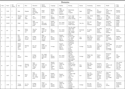
We developed a tripartite conceptual model organized around a hierarchy of concepts, domains, and measures. Concepts capture broad influences that will differentiate census tracts: population, environment, and economy. These broad concepts can be further disaggregated into domains; for example, population contains the domains of age, race, education, family structure, and language. In turn, each of these domains is connected to a set of measures from the ACS (see Table 2; note that the list of measures is not inclusive).

Table 2. Geodemographic conceptual model

Concepts	Domains	Measures
Population
	Age	Age distributions
	Race	Racial categories
	Education	High school graduate, college degree, professional degrees
	Family structure	Same-sex couples, married couples, single females with children
	Language	Only speak English, Spanish at home (with or without good English)
Environment
	Stability	Moved within a year (same town or from another town)
	Housing	Vacancy, structure type, building age, home values, rent
	Density	Population density
Economy
	Commuting	Duration (e.g., 25–29 minutes), commuting by public transport
	Occupation	Types of employment (e.g., agriculture, retail, etc.)
	Wealth	Income, public assistance, vehicle ownership

The selection of domains, concepts, and measures is a somewhat subjective exercise, but doing so appropriately is part of the art of building geodemographic classifications. The following sections provide the rationale behind our selection of concepts, domains, and measures. A full list of the variables considered during the creation of the classification and a complete data file are available online (http://doi.org/10.3886/E41329V2).

Population

Although the United States in the aggregate is becoming more diverse, at the census tract scale, significant racial, ethnic, and economic segregation persists (Fryer and Katz 2013; Logan 2013). Language can be a key indicator of these differences (Beckhusen et al. 2013), and we include the ability to speak any language other than English and the percentage of the population who speak Spanish and have low English proficiency as variables within the classification. In addition to spatial variation by race, there are important regional differences in the age structure of populations. High numbers of young or old people relative to the taxpaying working-age population can stress social service systems like education and health care. In 2010, Utah had a very high number of children per working-age adult, whereas Washington, DC, had fairly low numbers of children per working-age adult (Howden and Meyer 2011). Historically, in the United States, geographic and racial differences in family structure have been used to describe a wide variety of social outcomes. Especially for children, family structure seems to affect health as well as educational and behavioral outcomes, particularly for children raised by single mothers (Matsueda and Heimer 1987; Astone and McLanahan 1991; Montgomery, Kiely, and Pappas 1996). Although spatial patterns in family structure have received little recent attention in the literature, it seems intuitive that they persist, with, for example, relatively fewer married couple households with children living within the dense metropolitan cores. Similarly, for education, we are not aware of generalizable spatial patterns in educational attainment, but the literature makes it clear that education is an important predictor of well-being and socioeconomic status (Cutler and Lleras-Muney 2010).

Environment

The environment concept contains elements of the built and social environment. The built environment not only describes the physical look and feel of a place, but it also greatly affects the attractiveness of places to various types of people (Salesses, Schechtner, and Hidalgo 2013). Factors such as the design, age, vacancy rate, and value of buildings are all important signals about the nature of places to visitors and are highly correlated with economic and social factors. Some elements of the built environment, such as vacancy, affect crime and the perception of safety (Sampson, Morenoff, and Gannon-Rowley 2002). The density of the built environment is also an important correlate of travel behaviors and physical activity (Ewing and Cervero 2001; Handy et al. 2002; Papas et al. 2007). On the social side, neighborhood stability is related to a variety of social and economic outcomes (Sampson, Raudenbush, and Earls 1997; Temkin and Rohe 1998). Residential stability is a vague term; here we measure it as intracity residential moves and inmigration. Areas that are attractive to inmigrants and areas that have short tenure in housing units (high turnover) have low rates of residential stability, however intra- and intercity moves suggest a different causal mechanism; thus, we differentiate these types of neighborhood instability.

Economy

We define economy broadly to include household wealth (income, home values), employment by industrial sector, and descriptors of commuting behavior. Spatial variation in economic activity and household wealth is an important element of intra- and intermetropolitan variations in social landscapes (Fischer 2003). Specifically, we measure this concept over the domains of wealth, industry of occupation, and commuting. Perhaps to a greater extent than some of the other concepts, however, the measures that comprise this domain are related to many other domains; for example, the relationship between income and race (Ross, Nobrega, and Dunn 2001), industry type and geographic location (Moretti 2012), or transport mode and urban form (Buehler 2011).

Selecting and Calibrating Variables

The translation of concepts and measures into domains is not trivial, as 2,864 ACS variables corresponding to the broadly defined domains (Table 2) were considered (the full data file is available online at http://doi.org/10.3886/E41329V2). Although the ACS estimates are available down to a block group level (between 600 and 3,000 people), at this scale, the data become highly uncertain. Census tracts, which generally have between 1,200 and 8,000 people, with a target of 4,000 people, are used in this classification because they represent a balance between geographic detail and attribute precision. Tracts with fewer than 100 people were excluded from the analysis.

There are competing views about how correlation between input variables should be handled in clustering applications. One approach is to use principal components analysis to reduce the number of variables down to a set of uncorrelated components. R. J. Harris, Sleight, and Webber (2005) argued that this has the potential to mask nonlinear or spatially varying relationships between variables. Spatial variants of principal components analysis, such as geographically weighted principal component analysis (P. Harris, Brunsdon, and Charlton 2011), might provide an answer to this critique. A simple strategy is to drop correlated variables. Vickers and Rees (2007) argued that such removals have to be on the basis of individual merit and that blanket rules are not really appropriate. One issue we foresee with excluding variables on the basis of using correlation is that those relationships between variables would not necessarily be geographically homogenous and, through exclusion, there would be a risk of reducing important interactions that might differentiate areas. A third approach is weighting variables. R. J. Harris, Sleight, and Webber (2005) discussed how in the development of a commercial geodemographic classification, correlation was allowed. Highly correlated variables were down-weighted, however, to reduce their impact on the classification.

The general concern about correlated variables arises because many clustering methods rely on distance metrics, like Euclidean distance, to measure the similarity among observations. In clustering applications, the similarity among places is often measured by a distance metric of the form where represent the difference between two observations, or one observation and the centroid of a cluster, for the p variables in the model. Increases in are interpreted as increases in dissimilarity. Due to the additive nature of similarity calculations, small changes in a correlated set of variables can have a larger impact on similarity calculations than more significant changes in an uncorrelated set. If, for example, a classification was built using three variables that measured the housing market and one variable that measured socioeconomic status, and if the housing market variables were correlated with each other, small changes in the three housing market variables would have a larger net effect on similarity calculation than a much larger change in the single socioeconomic status variable. Thus, the final classification would more effectively differentiate small variations in the housing market than changes of a similar magnitude in socioeconomic status. The story is not quite that straightforward, however, because the amount of variance in a given variable or set of variables matters as well, as those with higher variance are more influential (Magidson and Vermunt 2002). In geodemographic analysis, correlation in the input variables does not lead to “incorrect” typologies. Geodemographic classifications cannot be true or false; they can only be good or bad relative to the purpose for which they were created. Openshaw, Cullingford, and Gillard (1980) noted, “[a] classification can only be deemed ‘good’ or ‘poor’ when it has been evaluated in terms of the specific purpose for which it is required; there is no magic universal statistical test that can be applied” (p. 421).

Avoiding correlation in any sort of complex geographic analysis is very difficult, whether one looks to David Tobler or Waldo Harvey: The idea that “everything is related to everything else” (Harvey 2010, 303) seems to be a common maxim in geographic inquiry (Tobler 1970). Accepting the inevitability of correlation among variables, we attempt to manage it by ensuring that domains are relatively balanced so that one domain does not disproportionally influence the results. Practically, this ensures that calculation of similarity (s), and thus the classification, is not overly influenced by a single domain. This largely subjective process was guided by statistical descriptions of the input data (summarized later) and was complicated by the fact that the correlated measures often logically belong to more than one domain. Rather than using only statistical tools to guide variable selection, our approach emphasized the utility of the final classification. That is, we wanted to avoid a situation, like the example in the previous paragraph, where one set of correlated variables drove the results and the classification failed to capture meaningful variation across the domains of interest. Although it is hard to prove that a classification is “correct,” we demonstrate the utility of our framework and our model by demonstrating that the classification is capable of differentiating patterns in two diverse data sets.

Variables were evaluated within the context of the framework in Table 2. The goal was to select variables that measured each domain, taking into account practical considerations such as coverage, margins of error, redundancy with other variables in the model, and balancing of domains. With regard to the first two of these criteria, rather than employ rigid rules, we selected variables with reasonable precision and near universal coverage. This is complicated by the fact that the quality of variables is not uniform: Some places have fairly good estimates of the percentage of commuters who use public transit, but in other places the margins of error are so high that estimates are essentially unusable (Spielman and Folch 2014). Some variables were deemed important (e.g., the number of same-sex couples) and were retained in the analysis, even though the coverage was less than universal and margins of error were often quite high by comparison. The handling of noncomplete cases is described in the later sections. Through this manual process, we refined the set of 2,864 variables down to 136 variables. This left 3,535 of 74,001 tracts with at least one missing value. A description of each variable and its origin (ACS table number) is available online (https://github.com/geoss/acs_demographic_clusters). Pairwise Pearson correlation coefficients ranged from r = 0.976 for the correlation between the percentage of population that speaks Spanish and the percentage of the population that self-identifies as Hispanic or Latino to r = 0.00045 for the correlation between the percentage of population that identifies as American Indian or Alaska Native and percentage Hispanic or Latino. Multiple correlations were calculated by regressing each input variable on all other input variables (excluding variables that summed to 100 percent, such as the percentage of population in each age cohort). These multiple correlations ranged from r² = 0.98 for the median value of owner-occupied housing units to r² = 0.03 for the percentage of same-sex (female) couple households.

A final processing step was to standardize variables. Tarpey (2007) suggested that the optimal transformation for cluster analysis is one in which the between-cluster variance is maximized. For useful review of standardization procedures, see R. J. Harris, Sleight, and Webber (2005) and Vickers (2006). There is some evidence to suggest that the use of the z score is not the most effective solution for k-means (Steinley 2004). Following this review, and in line with procedures used in prior national open geodemographic classification (Vickers and Rees 2007), we implemented a range standardization of the input variables that scales each variable between zero and one.

Identifying Types of Tracts

There are dozens of algorithms that could potentially be used to build a geodemographic classification (Spielman and Thill 2008; Adnan et al. 2010). In general there has been little work on how uncertain input data affect classification, and few algorithms for uncertain input data exist (Cormode and McGregor 2008). Those algorithms that do account for uncertainty view the input data as an n-dimensional region (a probability distribution function) as opposed to discrete points in n-dimensional space (e.g., Ngai et al. 2006). The frequent occurrence of zero estimates in the ACS complicates the application of these methods because uncertainty around these zero estimates is not adequately captured by the margins of error reported by the ACS (these yield negative counts). It is not possible given the current state of the public use data to specify a probability distribution function for the ACS tract-level data.

To facilitate methodological transparency and reproducibility, we opted to use simple and widely available methods. Our classification is built using the k-means and Ward's hierarchical clustering algorithms. Within the context of geodemographic classification, Adnan et al. (2010) illustrated the efficiency of k-means relative to some other more modern algorithms. The use of k-means to build a geodemographic classification can be implemented in two different ways. In the top-down approach, a small number of clusters are initially created to partition the input data. Then these initial clusters are subdivided again using k-means. This procedure yields a hierarchical classification (as in Vickers and Rees 2007). The alternate is to create the classification from the bottom up. This approach is commonly implemented in commercial classifications (R. J. Harris, Sleight, and Webber 2005). In this approach, the initial step is to create a typology with many clusters, which forms the “bottom” level of the classification. For example, in the United Kingdom, the Mosaic classification from Experian can be supplied at a segment level of 252 clusters; likewise, in the United States, PSYTE Advantage from Pitney Bowes is built up hierarchically from around 400 small clusters, which they refer to as atoms. This large number of bottom-level clusters is then aggregated into coarser groupings using a hierarchical clustering algorithm.

Selection of the most appropriate k values for the bottom level is typically done using a mix of subjective and objective criteria. We built a bottom-up classification with k = 250; although this number is arbitrary, it is broadly consistent with the commercial classifications (e.g., Mosaic and PSYTE). Because k-means is sensitive to starting conditions, the algorithm was randomly initialized 100,000 times. Each run of k-means was allowed a maximum of 1,000,000 steps. The data input for the k-means analysis was a matrix of range standardized data comprising 70,466 rows (tracts) with attributes for 136 columns (variables). The fit of a k-means solution can be calculated by summing the distance between each observation and its nearest cluster centroid. Using these criteria, the best fitting solution was selected, with the final result being more than 3 SD better than the average of the 100,000 runs. As noted earlier, 3,535 rows of data were excluded, as they had at least one missing value. These records were assigned a cluster postclassification by calculating the Euclidean distance between the nonmissing values and all cluster centroids. Observations with missing data were then assigned to the nearest cluster centroid.

Following k-means, a Ward's hierarchical cluster analysis was implemented on a k × p matrix of cluster centroids, where the centroids were defined as the classwise mean of the m input variables. Ward's uses a k × k distance matrix that specifies the dissimilarity of each observation (centroid) to all other observations (centroids). The elements of this matrix are successively combined in n − 1 agglomerative steps in which observations are merged until a single group is formed from the 250 input centroids. In Ward's method, grouping decisions are made on the basis of minimizing the increase in an objective function that measures within-group variance (Kaufman and Rousseeuw 1990). The merging process can be visualized using a dendrogram (Figure 1). In a dendrogram, the height of the connecting lines gives an indication of separation between clusters with various levels of partition (Everitt 2011). Figure 1 shows the 250 clusters, generated by k-means at the bottom, as the algorithm has progressed. The branches of the dendrogram can be seen to represent progressively larger aggregations of the initial 250-cluster input.

Figure 1. Dendrogram showing the 250 classes created via k-means and how they are combined into ten groups.

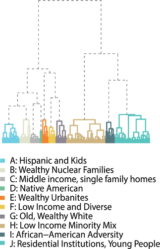
To create coarser levels of the classification, the dendrogram in Figure 1 could be cut into anywhere from 2 to 249 distinct groups of tracts by drawing a horizontal line through the figure. Determining the quality of each of these possible groupings is essential. Average silhouette width is a statistic that can be used to diagnose the quality of each possible cut of the dendrogram (Kaufman and Rousseeuw 1990). Silhouette width is calculated as a ratio of within-cluster homogeneity or compactness to the separation between clusters ( ) where a_i is the average Euclidean distance of data point i from other points assigned to the same cluster and b_i is the Euclidian distance of point i from the nearest (i.e., most similar) cluster to the one to which i is assigned. When the difference between a_i and b_i (s_i) is large, the ith observation is assigned to a distinct group that is well separated from the other groups. If s_i is negative, observation i is misassigned; that is, it is more similar to members of cluster b than cluster a. The scores range from –1 to +1, with positive scores representing good solutions. We calculate the s_i for each of the more than 74,000 tracts and then take the average for 2 to 249 cuts of the dendrogram (Figure 2). Although other cuts of the dendrogram were justifiable, on the basis of a preference for parsimony, we cut the dendrogram to yield a final two-level classification of ten and fifty-five nested clusters. The base of Figure 1 is colored according to the ten-class cut of the dendrogram. The descriptive labels and the properties of each group are summarized in Figures 3, 6, 7, 8, and 10.

Figure 2. Average silhouette for partitions of the 250-class k-means solution. Vertical lines indicate the ten-class group level of the classification and the fifty-five-class type level of the classification.

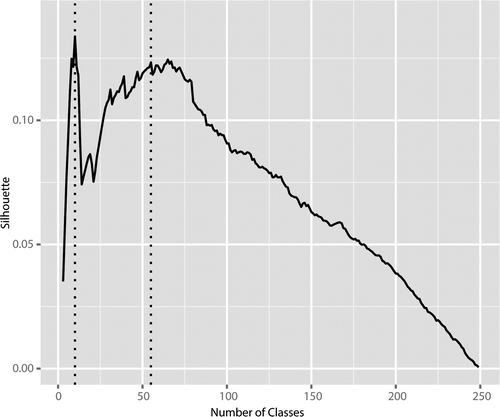
Figure 3. Summary of the ten-class group level of the classification by domain.

Results: A Sociospatial Classification of the United States

The highest level of the classification features ten clusters that are referred to as groups. The next level breaks these ten groups into fifty-five clusters referred to as types. Figure 3 describes the group level of the classification, Figure 4 maps the groups in Chicago and New York City, and Figure 5 shows the groups for the entire United States. To facilitate description, we compute index scores for each variable in the classification (), which rescales each variable such that a value of 100 represents the national mean, a value of 200 is twice the national average, and a value of 50 is half the national average. Simply stated, index scores measure the percentage of the national average for each variable. Figures 6 through 8 show these index scores for measures (variables) by domain for the highest level of the classification (groups) and Figure 3 summarizes these figures. The rightmost column of Figure 3 contains a brief descriptive label for each group, which is used in cartographic products (e.g., Figures 4 and 5). Labels for such a multidimensional classification seem excessively reductionist, and it is difficult to describe variation across many attributes in a few words. Rather than a lengthy verbal description of each class, we encourage the reader to study the figures to get a sense of the classification.

Figure 4. Group level (ten-class) map of census tracts in New York City and Chicago (maps not to scale).

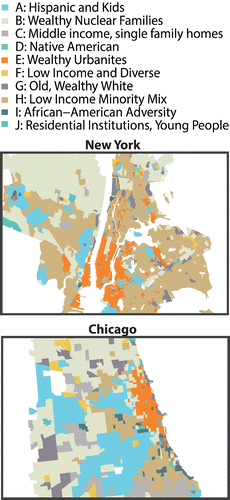
Figure 5. Group-level (ten-class) map of census tracts in the United States.

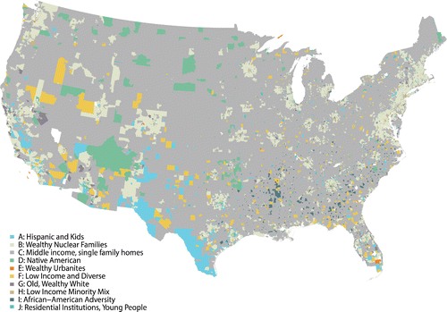
Figure 6. Variables from the population domain by group. Numbers represent the percentage of the national average for each variable in each group. For example, the top cell in Panel A indicates that in Group J the number of people with less than a high school education is 72 percent of the national average.

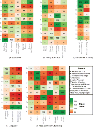
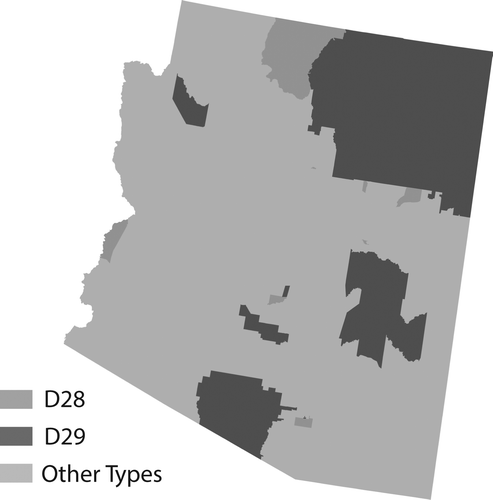
Groups vary substantially in size. The smallest, Group D, contains 367 tracts that are mainly concentrated on Native American reservations in Arizona, New Mexico, the Dakotas, and Oklahoma. Group D contains an index score of 5,995 for Native Americans, meaning that the percentage of the population that is Native American is more than fifty times the national average (see Figure 8E). Furthermore, Group D contains two types that are differentiated by both location and demographics. The first type (D28) contains an index score of 10,108 for Native American and contains the core areas of large reservations in Arizona (see Figure 9) and the Dakotas. The second type (D29) of Group D contains tracts in a large sections of eastern Oklahoma and scattered tracts in the interior and coasts of the United States. These tracts contain more middle-class households and have a smaller, but still substantial, percentage of the population who identifies as Native American (Native American index score = 3,870).

Figure 7. Variables from the economy domain by group. Numbers represent the percentage of the national average for each variable in each group. For example, in Panel B the 493 in the leftmost column indicates that the number of people without a car in Group E is 493 percent of the national average.

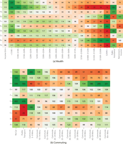
Figure 8. Housing variables form the environment domain by group.

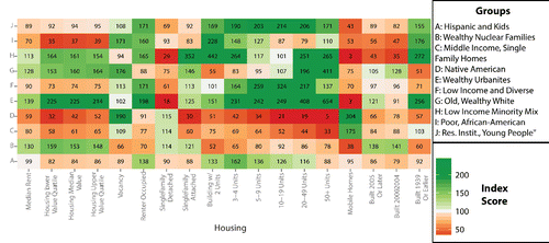
Figure 9. The type level of the classification for Group D in Arizona.

The largest of the groups within the classification is Group C, which contains 28,625 tracts and dominates Figure 6 given that it contains wide expanses of rural areas of the United States. This group is diverse geographically but is generally characterized by low residential densities and an older, low-income, English-only-speaking population (see Figure 8A). There is significant geographic diversity within this group, including an urban type consisting of tracts in older Rust Belt cities characterized by single-family housing, and a rural type characterized by agricultural employment. Many of the types in Group C have populations greater than the entirety of Group D. Within some groups, such as C, there is quite a bit of demographic variation. Although this intragroup diversity is less than desirable, it is the cost of parsimony. The fifty-five type levels of the classification provide more intraclass homogeneity at the cost of significant complexity.

Group B captures much of the stereotypical U.S. suburban landscape, containing places where relatively wealthy families with children live in single-family houses. Most metro areas in the United States are surrounded by areas belonging to Group B. This group is characterized by commutes of between thirty and ninety minutes, high housing costs, and high levels of education. This group has eleven subtypes that capture regional variation in home prices, commuting time, the age of housing, and citizenship. It is notable that there are very few young adults between the ages of eighteen and twenty-four within Group B (see Figure 10)—this age group is either not living at home, residing independently outside these suburban areas, or possibly attending university.

Figure 10. Population pyramids showing age distribution by gender for each group of the classification. Bars show five-year age intervals. The width of the bar denotes the amount of variation within each age category in each group. The vertical tick on each bar denotes the median for each age interval. Note the very large numbers of young people in Group J and the inverted pyramid in Group G.

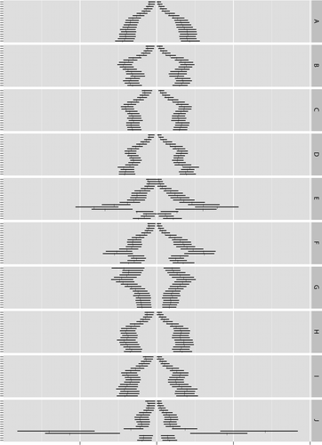
However, young adults (between the ages of eighteen and twenty-one) dominate Group J with an index score in excess of 500. This group is characterized by low incomes, short commutes, and a large number of people in group quarters (index score = 869). This group captures residential institutions such as college campuses that contain large numbers of young adults (see Figure 10). Group E is also dominated by young people, although they are slightly older than Group J. The age groups between twenty-two and thirty-five have index scores of around 200. Group E contains highly educated, young, wealthy, urban professionals. Group E also has very high population density (index score = 503), and the index score for the percentage of the population living in a building with fifty or more housing units is 654. Furthermore, Group E also has high residential mobility, with twice the national average for within-city and between-city moves. The racial composition of the class reflects the national average, with one exception, in that it has more than twice the average proportion of Asians. Residents of Group E have a high propensity to work in creative industries and additionally the highest number of same-sex couples.

A full enumeration of the groups and type characteristics would run into dozens of pages, and we urge readers to explore the accompanying website, figures, and code and data repository. The preceding discussion aims to illustrate that the classes identified represent coherent types of neighborhoods. This classification is “open” in the truest sense of the word, however, and by fully publishing all input data and analytical code we hope that users will not only be able to reproduce these results but will also be able to refine or adapt the classification.

Validation of the Typology

The grand challenge for geodemographic systems generally, and this classification in particular, is substantiating that the divisions they contain are something other than chance groupings in the data; that is, the structure of the classification mirrors the structure of society in some meaningful way. An important critique of such classifications is that geographic variations in behavior, health, and well-being are not necessarily determined by tract-level characteristics. Miller (2007) argued that the significance of place of residence might be decreasing in people's lives and that overemphasis on residential location leads to the risk of a place-based fallacy. On the other hand, Boardman et al. (2001), Sampson and Raudenbush (2004), and others have found place to be a powerful (and persistent) marker of inequalities and access to opportunities. Matthews (2008) noted that people's attachments to place are “polygamous” and suggested that area of residence is just one of many places that are important for people's lives. In recognition of the importance of such critiques, we conduct a robust endogenous and exogenous validation. The internal validation is designed to assess the differentness of the classes in the cluster solution, and the external validation is designed to show that there are, in fact, meaningful differences in social and behavioral outcomes between the groups in the classification.

Milligan and Cooper (1985) identified more than thirty statistical metrics for evaluating a cluster analysis. We calculate a Gini index (G) following the procedure outlined in Brown (1994) for each variable (v). The Gini index has been demonstrated elsewhere as a useful technique for evaluating geodemographic classifications (Batey, Brown, and Pemberton 2008; Petersen et al. 2011). The Gini index for a given variable (G_v) can be understood as the concentration of a particular variable within a particular group or type. A high G_v would mean that a measure is focused within a few groups or types, and low G_v means that the variable is evenly distributed across groups or types. For example, one of the lower Gini scores is for the measure “number of white people,” as whites are present in all groups and types. In theory, G_v is scaled between 0 and 1: A score of G_v = 0 would be a variable equally distributed over the clusters and a score of 1 would be for a variable found only in a single cluster. Because our clusters are different sizes, however, these theoretical maxima and minima are misleading. A synthetic Poisson random variable with constant λ assigned to all tracts results in a measure that occurs with an equal likelihood in all members of each group, and a variable such as this has a G_v = 0.08. A synthetic Poisson variable assigned only to all tracts in the largest group (28,265 tracts) has G_v = 0.68, and the same variable assigned to only the smallest group (367 tracts) has G_v = 0.99. For a group with 1,558 tracts, the same Poisson random variable yielded a Gini of G_v = 0.96. For the purposes of this evaluation, Gini scores in excess of 0.5 can be considered an indicator that a variable is relatively well concentrated within a particular cluster.

Several measures have exceptionally high G_v. Within the industry domain, employment in agriculture, forestry, fishing, and hunting and mining is concentrated within Groups A, C, and D. Commuting by public transit within the mobility domain and having no car within the wealth domain both have a high G_v and are found in Groups E, H, and I (see Figures 7–9). The internal G_v scores show that the variables are not evenly distributed across the classes and thus the classes are different from each other.

We conducted a further evaluation with data that are entirely exogenous to the input data. The exogenous evaluation aims to show that the categories represented in the geodemographic system are, in fact, meaningful sociospatial divisions by demonstrating the classification's ability to differentiate social phenomena. Two data sets, exogenous to the input data, are used to assess the extent to which the classification differentiates individual behavior and neighborhood context. A public domain individual-level data set profiling behavior was difficult to identify, but in the spirit of an open classification, and for reproducibility, we felt that it was important for all of the data that we used to be publicly accessible. The U.S. FEC Campaign Finance Disclosure Data contains all campaign contributions greater than $250 and describes the residential address (ZIP code) and the profession of the donor (FEC 2013).² The FEC data from 2007 and 2008 were used for this analysis because they captured an important election and fell within the period covered by the 2007 to 2011 ACS. The FEC data contain more than 3.3 million records and allow us to profile both individual self-reported profession and behavior (donations) by group. The second data set aims to profile neighborhoods and contains frequencies of all crimes for the approximately 800 census tracts in the City of Chicago for the twelve months prior to June 2012 (City of Chicago 2013). These data describe the context of neighborhoods, as the amount and type of crime in a tract is an important indicator of neighborhood conditions.

The exogenous evaluation used the same G_v statistic as the internal evaluation, with the aim of determining whether behaviors, professions, or crimes are concentrated in particular groups or types. In addition, one-way analysis of variance is used to assess the statistical significance of the differences in the group-level means for each variables. The results are indicated in addition to the G_v statistics and index scores in Table 3.

Table 3. Exogenous evaluation: Gini coefficient and index scores for Federal Election Commission profession and contribution amount

	Gini	Group A	Group B	Group C	Group D	Group E	Group F	Group G	Group H	Group I	Group J
Creative	0.68	28	160	22	7	1,031	45	221	68	17	126
Legal	0.59	32	165	30	11	784	74	217	51	36	112
Donations of $5,000 or more	0.59	34	166	31	44	717	71	299	29	27	115
Student	0.58	35	163	30	8	720	73	200	66	24	238
Professor	0.57	21	166	38	7	480	91	159	61	30	421
Donations of $1,000 or more	0.54	36	177	35	30	550	72	280	34	27	102
Finance	0.52	33	180	38	26	577	68	206	44	25	90
Farmer	0.48	112	64	152	202	32	53	78	1	61	58
Home maker	0.48	30	185	51	28	276	76	273	17	35	104
Engineer	0.44	40	210	45	24	195	85	142	27	20	80
Higher professionals	0.43	40	171	50	30	434	81	203	32	36	95
Donations of $250–$1,000	0.43	37	172	52	33	386	80	225	36	31	114
Retired	0.42	34	160	62	49	236	79	359	23	26	129
Medical	0.38	51	164	61	31	244	99	195	28	42	126

* p < 0.001, one-way analysis of variance on group-level means.

Table 4. Crime in Chicago

	Gv	Group A (%)	Group B (%)	Group C (%)	Group D (%)	Group E (%)	Group F (%)	Group G (%)	Group H (%)	Group I (%)	Group J (%)
Manslaughter	0.73	62	0	0	—	0	0	0	278	0	0
Gambling	0.69	8	6	79	—	2	10	9	276	218	0
Prostitution	0.63	90	7	37	—	31	19	13	200	150	79
Drug abuse	0.61	47	16	82	—	32	4	40	221	189	43
Homicides	0.58	61	30	114	—	15	18	16	193	183	0
Weapons violation	0.57	51	18	139	—	24	6	37	193	227	28
Aggravated battery	0.56	61	28	96	—	44	16	45	187	212	83
Disorderly conduct	0.55	82	34	83	—	50	10	44	169	174	48
Public violence	0.55	51	30	146	—	43	5	48	182	193	65
Arson	0.55	104	42	65	—	21	0	29	150	225	60
Aggravated assault	0.54	65	33	114	—	52	18	60	171	213	43
Family offenses	0.54	83	42	94	—	49	21	59	162	157	72
Violent	0.53	60	35	117	—	70	12	65	172	189	125
Battery	0.53	62	38	99	—	69	21	68	173	202	105
Liquor license	0.52	137	88	20	—	145	49	0	87	127	115
Robbery	0.51	57	40	131	—	92	10	79	164	168	162
Sexual assault	0.50	67	39	108	—	91	0	71	160	171	358
Assault	0.50	62	42	115	—	89	21	77	159	203	133
Burglary	0.50	75	61	110	—	99	19	48	146	147	66
Misc. offense	0.49	64	44	99	—	105	24	63	157	206	187
Vandalism	0.49	79	55	111	—	87	30	69	141	166	95
Vehicle theft	0.47	95	68	97	—	102	27	68	122	144	108
Stolen property	0.46	104	61	112	—	90	0	64	104	231	0
Sexual abuse	0.46	96	62	77	—	118	33	78	121	157	291
Property	0.42	69	65	100	—	197	29	90	122	146	326
Forgery	0.40	68	51	114	—	217	26	113	115	125	776
Embezzlement	0.39	69	53	105	—	206	257	0	116	99	899
Fraud	0.38	46	57	96	—	282	15	108	127	154	562
Larceny	0.38	60	66	98	—	253	33	110	115	146	466
Percentage of population		32	14	10	0	7	1	1	28	4	0.1
Percentage of crime		20	7	11	0	9	0.3	1	43	6	0.8

Note: This table shows G_v for each type of crime. Cells contain the percentage of the city-wide crime rate. Values greater than 100% indicate more crime than average and values less than 100% indicate less crime than average. The bottom rows show the percentage of the city's population that lives in each group and the percentage of all crime that occurs in each group. Group D does not occur in the city.

Table 3 shows G_v for elements of the FEC data and the index score for each group. Some grouping of professions was necessary; for example, the top row, “Creative,” includes individuals who identified themselves as working in one of twenty-eight professions.³ Individuals who worked in creative fields were shown to be concentrated within Groups E and H—index scores of 248 and 192, respectively—both of which are high-density urban classes. Creative professionals are nonexistent in Group D, which is a rural class dominated by Native Americans, but for Group D the profession of farmer has an index score of 500 in the FEC data. Large donations (more than $5,000) are concentrated in Groups E and F and, interestingly, both of these groups are characterized by households with few children and more than twice the national average for households making more than $200,000 per year. For larger donations, G_v tended to increase, which would reflect a small number of givers resident within more affluent groups, mirroring the larger G_v observed for tracts with populations of high earners within the endogenous evaluation. Further support for the efficacy of the classification is illustrated by professors and students being concentrated within Group J, which includes large residential facilities (group quarters) like colleges and universities.

The second validation data set was downloaded from the City of Chicago and counts the occurrence of twenty-nine different types of crimes in each census tract of the city. Gini scores (G_v) range from 0.38 for larceny to 0.73 for manslaughter (see Table 4). Interestingly, 62 percent of all crime in the city is contained within two groups that collectively contain about 60 percent of the population. The distribution of crimes within these two groups, however, is startlingly unequal. Group H, which is characterized by low-income minority populations, contains 43 percent of all crime in the city, even though it contains only 28 percent of the total population. On the other hand, Group A contains 32 percent of the population but only 20 percent of the crime. For each type of crime, Table 4 shows the crime rate (per 100,000 people) in each group as a percentage of the city-wide average. For example, the homicide rate in Group C is 114 percent of the city-wide average (i.e., 14 percent higher than the city-wide rate). In Group H the crime rate for most crimes is higher than the city-wide average; for crimes like prostitution, drug abuse, manslaughter, and homicide, the crime rate is around twice the city-wide average. Comparing Group H to the relatively affluent Group B shows dramatic differences. The homicide rate in Group B is 5 per 100,000 people compared to 33 per 100,000 people in Group H, and 212 of the 381 homicides in the database occurred in Group H. Larceny (G_v = 0.38) and property crimes (G_v = 0.42), which account for about a third of all crimes in the database, are not concentrated within a particular type of neighborhood. On the other hand, rarer but more violent crimes like homicide (G_v = 0.58) and manslaughter (G_v = 0.73) tend to be concentrated in particular groups. These strong intergroup differences support the validity of the classification. From an operational perspective, the clustering of specific types of crime in specific types of neighborhoods provides useful information for law enforcement agencies; for example, geodemographically targeted campaigns might be more successfully in the mitigation of gambling or violence (which have high G_v) than for larceny (which has a low G_v).

Discussion and Conclusions

The changing reality of U.S. data demands a change in practice. As public statistics have become less precise, the ability to understand tract-to-tract demographic or economic variation using the variables paradigm is diminished. This article is rooted in a pragmatic effort to identify a way to study neighborhoods in the face of highly uncertain data. We argue that viewing census tracts as instances of different types of places is effective, given that measurement errors will likely be reduced for large ensembles of variables, thus allowing the identification of types of neighborhoods even though individual variables are highly uncertain. Through creation of a geodemographic classification for the United States, we make the case for a new mode of national tract-level analysis. The geodemographic approach conceptualizes sociospatial variation as a hierarchical typology that emerges through the nexus of many social, economic, and built environment attributes. Ultimately, the statistical details of the approach are secondary to its utility, and we briefly demonstrated the strengths and limitations of the classification, providing evidence of the classification's ability to provide logically consistent and practically applicable discrimination of types of places in two exogenous data sets.

Care has been taken to ensure that the measures we used as input to the classification are well grounded in the social scientific literature. We aimed to select a balanced set of variables that capture variance within a carefully selected set of concepts and domains. Attribute selection was constrained by practical concerns about completeness, correlation, and data quality. Furthermore, care was taken to ensure that all methods and data are freely available and open source, making both the methods and the results reproducible. All aspects of this project, including data and code, are within the public domain. We do not claim that the classification presented here is the definitive representation of U.S. sociospatial structure, but by being open and transparent in both data and methods, and by establishing a conceptual framework for such classifications, we hope to stimulate others to adopt and refine this geodemographic framework.

The problems motivating this article are not unique to the United States and are influenced by the changing nature of data economies in a number of countries where high-resolution census data are increasingly under threat (Shearmur 2010). Despite these concerns, however, there has been a dearth of research into how uncertain data affect our understanding of the social landscape and how to overcome these data limitations in applied research settings. The approach suggested here is but one of many possible ways forward; alternatively, one might focus on improving single variable estimates through augmenting public survey data with ancillary sources of information such as administrative records, or “big data” (Langford 2013). For example, Porter et al. (2014) illustrated how the language used in Google searches can improve census estimates of ethnic populations. The alternative approach taken here is to reduce the impact of imperfect variable estimates through assembly of a multidimensional typology. We believe that such contextual descriptors, although not ideal for all questions, have real advantages for examining social phenomena that vary noncontinuously across the socioeconomic spectrum and will gain increasing relevance in applications where uncertainty in the ACS is especially high.

Notes

1. There have been some recent methodological adjustments to the ACS in an effort to minimize these variations in data quality (see Sommers and Hefter 2014).

2. Extensive processing of the FEC data was, however, necessary, given that the data are available at the ZIP code level. This involved the manipulation of the ZIP code data into census tracts using a “crosswalk” lookup table developed and distributed by the U.S. Department of Housing and Urban Development (HUD 2013).

3. The list of “creative” professions is writer or director, museum director, graphic artist, art consultant, graphic design, poet, design, jewelry designer, film editor, film-maker, curator, film director, screenwriter, landscape designer, art director, songwriter, TV producer, sculptor, editor, writer or editor, landscape architect, creative director, graphic designer, actress, musician, actor, advertising, and art dealer.

References

- Abbott, A. 1997. Of time and space: The contemporary relevance of the Chicago school. Social Forces 75 (4): 1149–82.
- Adnan, M., P. A. Longley, A. D. Singleton, and C. Brunsdon. 2010. Towards real time geodemographics: Clustering algorithm performance for large multidimensional spatial databases. Transactions in GIS 14 (3): 283–97.
- Astone, N. M., and S. S. McLanahan. 1991. Family structure, parental practices and high school completion. American Sociological Review 56 (3): 309–20.
- Batey, P., P. Brown, and S. Pemberton. 2008. Methods for the spatial targeting of urban policy in the UK. Applied Spatial Analysis and Policy 1 (2): 117–32.
- Bazuin, J. T., and J. C. Fraser. 2013. How the ACS gets it wrong: The story of the American Community Survey and a small, inner city neighborhood. Applied Geography 45:292–302.
- Beckhusen, J., R. J. Florax, T. de Graaff, J. Poot, and B. Waldorf. 2013. Living and working in ethnic enclaves: English language proficiency of immigrants in US metropolitan areas. Papers in Regional Science 92 (2): 305–28.
- Boardman, J. D., B. K. Finch, C. G. Ellison, D. R. Williams, and J. S. Jackson. 2001. Neighborhood disadvantage, stress, and drug use among adults. Journal of Health and Social Behavior 42 (2): 151–65.
- Box, G. E. P., and N. R. Draper. 1987. Empirical model-building and response surfaces. New York: Wiley.
- Brown, M. C. 1994. Using Gini-style indices to evaluate the spatial patterns ofon of the performance of geodemographic classifications. Journal of the Royal Statistical Society, Series A 174 (1): 17–30.
- Brueckner, J. K., and S. S. Rosenthal. 2009. Gentrification and neighborhood housing cycles: Will America's future downtowns be rich? The Review of Economics and Statistics 91 (4): 725–43.
- Buehler, R. 2011. Determinants of transport mode choice: A comparison of Germany and the USA. Journal of Transport Geography 19 (4): 644–57.
- Citro, C. F., and G. Kalton. 2007. Using the American Community Survey: Benefits and challenges. Washington, DC: National Academies Press.
- City of Chicago. 2013. Crimes 2001–present. https://data.cityofchicago.org/Public-Safety/Crimes-2001-to-present/ (last accessed May 30, 2013).
- Cormode, G., and A. McGregor. 2008. Approximation algorithms for clustering uncertain data. In Proceedings of the Twenty-seventh ACM SIGMOD-SIGACT-SIGART Symposium on Principles of Database Systems, 191–200. New York: ACM.
- Cutler, D. M., and ACM. Lleras-Muney. 2010. Understanding differences in health behaviors by education. Journal of Health Economics 29 (1): 1–28.
- Ehrenhalt, A. 2012. The great inversion and the future of the American City. New York: Knopf.
- Environmental Systems Research Institute (Esri). 2013. Tapestry segmentation: Reference guide. http://www.esri.com/library/whitepapers/pdfs/community-tapestry.pdf (last accessed 22 July 2015).
- Everitt, B. 2011. Cluster analysis. 5th ed. Chichester, UK: Wiley.
- Ewing, R., and R. Cervero. 2001. Travel and the built environment: A synthesis. Transportation Research Record 1780 (1): 87–114.
- Fay, R. E., and G. F. Train. 1995. Aspects of survey and model-based postcensal estimation of income and poverty characteristics for states and counties. In Proceedings of the Government Statistics Section, American Statistical Association, 154–59. Alexandria, VA: American Statistical Association.
- Federal Election Commission (FEC). 2013. Contributions by individuals. http://www.fec.gov/finance/disclosure/ftp_download.shtml (last accessed May 20, 2013).
- Fischer, M. J. 2003. The relative importance of income and race in determining residential outcomes in US urban areas, 1970–2000. Urban Affairs Review 38 (5): 669–96.
- Fryer, R. G., and L. F. Katz. 2013. Achieving escape velocity: Neighborhood and school interventions to reduce persistent inequality. American Economic Review 103 (3): 232–37.
- Handy, S. L., M. G. Boarnet, R. Ewing, and R. E. Killingsworth. 2002. How the built environment affects physical activity. American Journal of Preventive Medicine 23 (2): 64–73.
- Hanlon, B. 2010. Once the American dream: Inner-ring suburbs of the metropolitan United States. Philadelphia: Temple University Press.
- Harris, P., C. Brunsdon, and M. Charlton. 2011. Geographically weighted principal components analysis. International Journal of Geographical Information Science 25 (10): 1717–36.
- Harris, R. J., P. Sleight, and R. J. Webber. 2005. Geodemographics, GIS and neighbourhood targeting. London: Wiley.
- Harvey, D. 2010. Social justice and the city. Athens: University of Georgia Press.
- Housing and Urban Development (HUD). 2013. HUD USPS ZIP code crosswalk files. http://www.huduser.org/portal/datasets/usps_crosswalk.html (last accessed June 30, 2013).
- Howden, L., and J. Meyer. 2011. Age and sex composition: 2010. Technical report, U.S. Census Bureau, Washington, DC.
- Kaufman, L., and P. J. Rousseeuw. 1990. Finding groups in data: An introduction to cluster analysis. New York: Wiley.
- Langford, M. 2013. An evaluation of small area population estimation techniques using open access ancillary data. Geographical Analysis 45 (3): 324–44.
- Lees, L., T. Slater, and E. K. Wyly. 2008. Gentrification. London and New York: Routledge.
- Logan, J. R. 2013. The persistence of segregation in the 21st century metropolis. City & Community 12 (2): 160–68.
- Longley, P., R. J. Webber, and L. Chao. 2008. The UK geography of the e-society: A national classification. Environment and Planning A 40 (2): 362–82.
- Lynch, K. 1960. The image of the city. Vol. 11. Cambridge, MA: Massachusetts Institute of Technology Press.
- Magidson, J., and J. K. Vermunt. 2002. Latent class models for clustering a comparison with k-means. Canadian Journal of Marketing Research 20:37–44.
- Matsueda, R. L., and K. Heimer. 1987. Race, family structure, and delinquency: A test of differential association and social control theories. American Sociological Review 52:826–40.
- Matthews, S. A. 2008. The salience of neighborhood: Some lessons from sociology. American Journal of Preventive Medicine 34 (3): 257–59.
- Miller, H. 2007. Place-based versus people-based Geographic Information Science. Geography Compass 1 (3): 503–35.
- Milligan, G., and M. Cooper. 1985. An examination of procedures for determining the number of clusters in a data set. Psychometrika 50 (2): 159–79.
- Montgomery, L. E., J. L. Kiely, and G. Pappas. 1996. The effects of poverty, race, and family structure on U.S. children's health. American Journal of Public Health 86 (10): 1401–05.
- Moretti, E. 2012. The new geography of jobs. Boston: Houghton Mifflin Harcourt.
- Navarro, F. 2012. An introduction to ACS statistical methods and lessons learned. Paper presented at the Measuring People in Place conference, Boulder, CO. http://www.colorado.edu/ibs/cupc/workshops/measuring_people_in_place/themes/theme1/navarro.pdf (last accessed June 20, 2014).
- Ngai, W. K., B. Kao, C. K. Chui, R. Cheng, M. Chau, and K. Y. Yip. 2006. Efficient clustering of uncertain data. In Data Mining, 2006. ICDM’06. Sixth International Conference, 436–45. Los Alamitos, CA: IEEE.
- Openshaw, S., D. Cullingford, and A. Gillard. 1980. A critique of the national classifications of OPCS/PRAG. Town Planning Review 51 (4): 421.
- Orfield, M. 1997. Metropolitics: A regional agenda for community and stability. Washington, DC: Brookings Institution Press.
- Papas, M. A., A. J. Alberg, R. Ewing, K. J. Helzlsouer, T. L. Gary, and A. C. Klassen. 2007. The built environment and obesity. Epidemiologic Reviews 29 (1): 129–43.
- Park, R., E. Burgess, and D. Roderick. 1925. The city. Chicago: Chicago University Press.
- Petersen, J., M. Gibin, P. Longley, P. Mateos, P. Atkinson, and D. Ashby. 2011. Geodemographics as a tool for targeting neighbourhoods in public health campaigns. Journal of Geographical Systems 13 (2): 173–92.
- Porter, A. T., S. H. Holan, C. K. Wikle, and N. Cressie 2014. Spatial Fay-Herriot models for small area estimation with functional covariates. Spatial Statistics 10:27–42.
- Ross, N., K. Nobrega, and J. Dunn. 2001. Income segregation, income inequality and mortality in North American metropolitan areas. GeoJournal 53 (2): 117–24.
- Salesses, P., K. Schechtner, and C. A. Hidalgo. 2013. The collaborative image of the city: Mapping the inequality of urban perception. PLoS ONE 8:e68400.
- Sampson, R. J., J. D. Morenoff, and T. Gannon-Rowley. 2002. Assessing “neighborhood effects”: Social processes and new directions in research. Annual Review of Sociology 28 (1): 443–78.
- Sampson, R. J., and S. W. Raudenbush. 2004. Seeing disorder: Neighborhood stigma and the social construction of broken windows. Social Psychology Quarterly 67 (4): 319–42.
- Sampson, R. J., S. W. Raudenbush, and F. Earls. 1997. Neighborhoods and violent crime: A multilevel study of collective efficacy. Science 277 (5328): 918–24.
- Shearmur, R. 2010. A world without data? The unintended consequences of fashion in geography. Urban Geography 31 (8): 1009–17.
- Shevky, E., and W. Bell. 1955. Social area analysis. Palo Alto, CA: Stanford University Press.
- Singleton, A., and P. Longley. 2009a. Creating open source geodemographics—Refining a national classification of census output areas for applications in higher education. Papers in Regional Science 88 (3): 643–66.
- ———. 2009b. Geodemographics, visualization, and social networks in applied geography. Applied Geography 29 (3): 289–98.
- Singleton, A., and S. Spielman. 2014. The past, present and future of geodemographic research in the United States and United Kingdom. The Professional Geographer 66 (4): 558–67.
- Sommers, D., and S. Hefter. 2014. Evaluating the impact of the 2011 sample reallocation for the American Community Survey. American Community Survey Research and Evaluation Report Memorandum Series, Report ACS14-RER-02, U.S. Census Bureau, Washington, DC.
- Spielman, S. E., and D. C. Folch. 2014. Reducing uncertainty in the American Community Survey through data-driven regionalization. PloS ONE 10 (2):e0115626.
- Spielman, S. E., D. Folch, and N. Nagle. 2014. Patterns and causes of uncertainty in the American Community Survey. Applied Geography 46:147–57.
- Spielman, S. E., and J.-C. Thill. 2008. Social area analysis, data mining, and GIS. Computers, Environment and Urban Systems 32 (2): 110–22.
- Steinley, D. 2004. Standardizing variables in k-means clustering. In Classification, clustering, and data mining application, ed. D. Banks, L. House, F. McMorris, P. Arabie, and W. Gaul, 53–60. Berlin: Springer.
- Tarpey, T. 2007. Linear transformations and the k-means clustering algorithm. The American Statistician 61 (1): 34–40.
- Temkin, K., and W. M. Rohe. 1998. Social capital and neighborhood stability: An empirical investigation. Housing Policy Debate 9 (1): 61–88.
- Tobler, W. R. 1970. A computer movie simulating urban growth in the Detroit region. Economic Geography 46 (Supp.): 234–40.
- U.S. Census Bureau. 2006. Design and methodology: American Community Survey. Technical Paper 67 (unedited version), U.S. Government Printing Office, Washington, DC.
- Vickers, D. 2006. Multi-level integrated classifications based on the 2001 census. PhD thesis, University of Leeds, Department of Geography, Leeds, UK.
- Vickers, D., and P. Rees. 2007. Creating the UK national statistics 2001 output area classification. Journal of the Royal Statistical Society, Series A: Statistics in Society 170 (2): 379–403.