Robust predictive compensation control for lateral magnetorheological semi-active suspension of high-speed trains with time delay

ABSTRACT

Aiming at reducing the effect of time delay on the control performance of magnetorheological (MR) damper semi-active suspension, a control strategy with strong robustness to time delay is investigated in this study, including the force controller of MR damper, the robust controller and the predictive compensator. The force controller of MR damper is built based on the hyperbolic tangent function; the robust controller is built based on the simplified model of car body lateral vibration and is designed by μ-synthesis method considering the effect of time delay; then the Smith predictive model and the lateral velocity predictor are designed, which form the predictive compensator of semi-active controller to reduce the effect of time delay. To validate the effectiveness of the proposed control strategy, several conventional semi-active controllers are designed as comparative objects. The simulation results show that the proposed semi-active control strategy can maintain good performance when time delay is in the range of 0–100 ms and has better robustness to time delay compared with the conventional control strategy.

KEYWORDS:

• High-speed train
• magnetorheological damper
• semi-active control
• robust control
• time delay

1. Introduction

As the core part of high-speed rail, high-speed trains (HSTs) play an important role in railway modernization. The suspension system of HSTs is very important to the handling stability and ride comfort of the train [1,2]. Generally, the suspension system can be divided into three types: passive suspension, active suspension and semi-active suspension. A large number of studies show that [3–5] the semi-active suspension can provide better performance with lower cost and complexity, which has advantages of less energy consumption, low cost and convenient maintenance.

The performance of semi-active suspension largely depends on the semi-active control strategy. The earliest research on semi-active control strategy can be traced back to the famous sky hook damper (SH) control proposed by Karnopp [6] in 1974. Subsequently, many semi-active control strategies based on SH control were proposed, including Rakheja-Sankar (RS) control [7], ground hook damper (GH) control [8], no-jerk SH control [9] and acceleration driven damping (ADD) control [10]. Meanwhile, a lot of advanced control methods are used in semi-active suspension control. Liao and Wang [11] used the semi-active LQG controller using acceleration feedback to control the 9-DOF vehicle model, and later extended it to the 17-DOF vehicle model [12]. Chen [13] applied generalized predictive control to semi-active suspension control. Zong et al. [14] designed a semi-active robust controller based on H_∞ theory, and verified that the controller can effectively suppress the lateral vibration of car body through the 17-DOF vehicle model.

In many studies, simulation results show that the semi-active suspension can achieve good performance. However, in practical application, due to the inevitable time delay from the signal collection, transmission, controller calculation, actuator response and so on, the actual control force deviates from the desired control force, which may greatly degrade the performance. Take magnetorheological (MR) semi-active suspension as an example, the time delay mainly comes from the response time of MR damper itself. The existing relevant research [15–18] shows that the response time of MR damper is about dozens to hundreds millisecond, and there are obvious differences in the response time for dampers of different models and sizes. Generally, the response time of large-size dampers will be relatively large.

In recent years, some scholars have studied the effect of time delay on semi-active suspension. Wang [19] pointed out that the effect of time delay on semi-active suspension and active suspension is different. For the former, time delay will only cause the change of vibration reduction performance, while for the latter, too large time delay will cause system instability. Cha et al. [16] studied the effect of time delay on buildings with large-size MR dampers when different control strategies are adopted. Qin et al. [20] gave a comprehensive analysis for the influence of controllable damper with time delay on different semi-active suspension control strategies based on the quarter vehicle model. Liao et al. [21] designed several semi-active controllers based on SH, ADD and Mixed SH-ADD control strategy, applied them to the 50-DOF model of HSTs and analysed the effect of time delay. The simulation results show that the performance will degrade with the increase of time delay, even worse than the passive control.

Scholars have done relevant research on the control strategy for semi-active suspension with time delay. Zhao et al. [17] designed a controller based on the fuzzy control strategy for the MR semi-active suspension and used the Smith predictive compensation method to compensate the time delay. However, this method needs obtain the road disturbance and the accurate model of the controlled object in advance, which is difficult to achieve in practical application. Zhang et al. [22] studied the semi-active control strategy of air suspension based on LMI and H_∞ theory, which has good robustness to parameter uncertainty and time delay. Wang et al. [23] proposed two Taylor series compound robust control methods to solve the time delay compensation problem of MR semi-active suspension.

At present, there have been many studies on the control strategy of active suspension with time delay, among which robust control is widely used [24–27], but studies on semi-active suspension are relatively few, especially for semi-active suspension of HSTs. Therefore, this paper investigates a control strategy to reduce the effect of time delay on the control performance of MR semi-active suspension of HSTs.

The structure of this paper is as follows. After the introduction, the 17-DOF model of HSTs is established and the track irregularity is numerically simulated in Section 2. In Section 3, based on the Bouc–Wen model, the dynamic model of MR damper is established as the actuator of semi-active suspension, and the MR semi-active suspension with time delay is built. In Section 4, the core part of this paper, a hyperbolic tangent model is proposed to fit the results of Bouc–Wen model, on which the force calculator and force controller of MR damper are established based. Then a simplified model of car body lateral vibration is established. Based on the simplified model, the robust controller is designed by μ-synthesis method after transforming time delay into model perturbation. Later, the Smith predictive compensation model is built based on the simplified model and the lateral velocity predictor is designed based on phase-lead compensator, which forms the predictive compensator together. In Section 5, the performance of the proposed control strategy is evaluated by simulation, and several conventional controllers are designed for comparison and analysis. The final conclusion of this paper is in Section 6.

2. Analytical model of HST

When studying the HST semi-active suspension control strategy, it is necessary to establish an appropriate dynamics model of HSTs, which needs to reflect the real situation as much as possible, but high complexity will make the design of the control strategy difficult.

In this paper, the 17-DOF dynamics model of HSTs (17-DOF model) is used to study the control strategy. 17-DOF model is a good choice with comprehensive consideration of control algorithm design and control performance analysis. And it is used wildly in the research about lateral vibration control of HSTs, due to including all lateral motion degrees of freedom for a single vehicle and reflecting lateral dynamic of the vehicle realistically.

The model assumes that the car body, bogie and wheel set are rigid, and considers the lateral, yaw and roll motion of the car body and two bogies, and the lateral and yaw motion of four wheelsets, which can basically reflect the actual lateral vibration of HSTs when driving on the track. The specific form of the model is described in Refs. [14,28]. Figure 1 shows the 17-DOF model using MR damper as secondary lateral adjustable damper, and Table 1 lists the input and output of the model. By comparing with the credible data from other published high-quality papers, the 17-DOF model built in this paper can be adopted, and the verification of it is presented in Appendix B.

Figure 1. 17-DOF dynamic model of HSTs with MR damper [14,28].

Table 1. Input and output of 17-DOF model.

	Output
Input	Component	Lateral	Yaw	Roll
Lateral alignment xy	Car body	yc	ψc	θc
Cross-level xθ	Front bogie frame	yt1	ψ t1	θt1
The front control force F1	Rear bogie frame	yt2	ψ t2	θ t2
The rear control force F2	Front bogie leading wheelset	yw1	ψw1
	Front bogie trailing wheelset	yw2	ψw1
	Rear bogie leading wheelset	yw3	ψw1
	Rear bogie trailing wheelset	yw4	ψw1

Random track irregularity is the primary cause of the vibration of HSTs, which can be regarded as the excitation input of dynamic model of HSTs. Meanwhile, the lateral vibration of HSTs is mainly caused by lateral alignment track irregularity and cross-level track irregularity. Therefore, in this paper, the lateral alignment track irregularity and cross-level track irregularity based on German low interference spectrum are selected as the track excitation of the model, and their power spectral densities (PSDs) are described as follows, respectively [29]. (1) $S_{\text{a}}\left(\Omega \right)=\frac{A_{\text{a}}{\Omega }_{\text{c}}^2}{({\Omega }^2+{\Omega }_{\text{r}}^{\text{2}})({\Omega }^2+{\Omega }_{\text{c}}^{\text{2}})}$(1) (2) $S_{\text{c}}\left(\Omega \right)=\frac{\left(A_{\text{v}}/b^2\right){\Omega }_{\text{c}}^{\text{2}}{\Omega }^2}{({\Omega }^2+{\Omega }_{\text{r}}^{\text{2}})({\Omega }^2+{\Omega }_{\text{c}}^{\text{2}})({\Omega }^2+{\Omega }_{\text{s}}^{\text{2}})}$(2) where Ω is the spatial frequency (rad/m); Ω_c, Ω_r and Ω_s are truncated frequencies (rad/m); A_a and A_v are roughness coefficients (m·rad) and b is half of the wheel rolling circle distance. The PSDs only describe the frequency domain characteristics of the track irregularity, and the time series describing track irregularity needs to be obtained according to (1) and (2) for simulations. In this paper, a trigonometric series method based on frequency domain sampling is used to simulate the irregularity signal [30].

3. MR semi-active suspension with time delay

The time delay of semi-active suspension can be divided into collection time delay and execution time delay [21]. Under the existing technical conditions, the time delay caused by signal collection, processing and transmission is negligible [36], so this paper only considers the execution time delay caused by the response time of the MR damper. Based on relevant material (see Appendix C), the achievable delay is determined as 0–100 ms.

In this paper, the modified Bouc–Wen model proposed by Spencer [31] is used to describe the dynamics of MR damper. And the specific form of MR damper with time delay is as follows: (3) $F=c_1\dot{y}$(3) (4) $\dot{y}=\frac{1}{c_0+c_1}[c_0\dot{x}+k_{0}x+\alpha z]$(4) (5) $\dot{z}=-\gamma |\dot{x}-\dot{y}|z|z{|}^{n-1}-\text{β}(\dot{x}-\dot{y})|z{|}^n+A(\dot{x}-\dot{y})$(5) (6) $\alpha ={\alpha }_a+{\alpha }_{b}I(t-\tau )+{\alpha }_c{I}^2(t-\tau )$(6) (7) $c_0=c_{0a}+c_{0b}I(t-\tau )$(7) where F is the damping force; I is the command current; c₁ represents the viscous damping at low velocities; c₀ represents the viscous damping at high velocities; x is the piston relative displacement; y is the internal displacement and z is the evolutionary variable; α, β, γ, n and A are parameters used to adjust the size and shape of hysteresis loop; τ is the response time delay, ranging from 0 to 100 ms. The best parameter values when the Bouc–Wen model is used to describe dynamics of MR damper are listed in Table 2.

Table 2. Parameter values of the modified Bouc–Wen model [14].

Parameters	Values	Parameters	Values
k0	0 N mm^−1	c1	91.6 N s mm^−1
c0a	8.4 N s mm^−1	β	0.15 mm^−2
c0b	11.23 N s mm^−1A^−1	A	4.5
αa	40 N mm^−1	γ	0.15 mm^−2
αb	2036.8 N mm^−1A^−1	n	2
αc	−535.95 N mm^−1A^−2

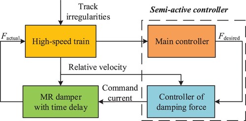
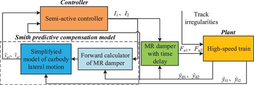
Figure 2 is the schematic of MR semi-active suspension with time delay, in which the MR damper with time delay generates the actual control force after receiving the command current calculated by the semi-active controller. However, there will be a deviation between the actual force and the desired because of time delay, which causes a degradation of control performance. To reduce the negative effect of time delay, a semi-active control strategy is proposed by combining the robust control and Smith predictive compensation method in this paper.

Figure 2. MR semi-active suspension system with time delay.

4. Robust predictive compensation control strategy

4.1. Force calculator and force controller of MR damper

The control force and command current are difficult to calculate through the Bouc–Wen model, while they are often needed in semi-active control strategy. Therefore, it’s necessary to establish the force calculator and force controller of MR damper. The former is used to calculate the output control force of MR damper, while the latter can calculate the command current to adjust MR damper.

The curve of hyperbolic tangent function is similar with the velocity force versus curve of MR damper, which can simulate the strong nonlinearity of MR damper with few parameters and high accuracy. Some scholars have described the dynamic characteristics of MR damper through hyperbolic tangent model [23]. In this paper, a modified hyperbolic tangent model is proposed to describe MR damper, as shown in (8), and the force calculator and force controller are established based on the model. (8) $F_{MR}=k_1\tanh [b_{1}v+b_2\text{sign}(a\left)\right]+k_{2}v$(8) where F_MR is the damping force (N), I is the command current (A), v is the piston relative velocity (mm/s), a is the piston relative acceleration, and k₁, k₂, b₁ and b₂ are the parameters to be fitted. To facilitate the solution of I, it’s assumed that k₁ and k₂ are functions of I, b₁ and b₂ are functions of the vibration state v_m of the damper, and v_m is defined as the root-mean-square (RMS) value of v in the last 1 s, as shown in (9). (9) $v_m\left(t\right)=\{\begin{array}{l}0,0\le t<1\\ \sqrt{{\int }_{t-1}^{t}v\text{(}t\text{)d}t},t\ge 1\end{array}$(9)

The parameters of hyperbolic tangent model are fitted through the simulation results of Bouc–Wen model. After a series of fitting, the specific forms of k₁, k₂, b₁ and b₂ are determined, as shown in (10) and (11). Table 3 lists the final fitting results. (10) $k_1=k_{10}{I}^2+k_{11}I+k_{12},k_2=k_{20}I+k_{21}$(10) (11) $b_1=b_{10}{v}_m+b_{11},b_2=b_{20}{v}_m+b_{21}$(11) Replace a by v(n)–v(n–1) and the force calculator is obtained based on (8) and parameters in Table 3, which takes the command current I, the velocity v(n) and v(n–1) as input and control force of MR damper as the output.

Table 3. Fitting results of the hyperbolic tangent model.

Parameters	Values	Parameters	Values
k10	–3818	b10	–1.58*10^−5
k11	9546	b11	0.02
k12	226.60	b20	8.26*10^−4
k20	9.28	b21	0.61
k21	7.52

Then apply the hyperbolic tangent model to the force controller. It’s clear that when the vibration state of MR damper is certain, if I = I_max, F = F_max; if I = I_min, F = F_min, which means the damping force F can change from F_min and F_max. In this paper, I_max= 1_, I_min= 0. And the solution of command current is divided into the following two cases:

Case 1: When the desired control force F_i ∈[-∞, F_min)∪[F_max, +∞), or F_i∈[–∞, F_max)∪[F_min, +∞), F_i cannot be completely tracked and can only be approached as close as possible. Let e₁= |F_i–F_max |, e₁= |F_i–F_max |, and I is determined through e₁ and e₁: when e₁≥ e₂, I = I_min; e₂>e₁, I = I_max.

Case 2: When the desired control force F_i ∈[F_min, F_max], or F_i∈ [F_max, F_min], the command current can be obtained by solving a quadratic equation with one variable based on (16). The specific form is as follows: (12) $I=\frac{-b+\sqrt{b^2-4ac}}{2a}$(12) (13) $\lambda =\tanh \left\{b_{1}v\right(n)+b_2\text{sign}[v\left(n\right)-v(n-1)\left]\right\}$(13) (14) $a=\lambda k_{10}$(14) (15) $b=\lambda k_{11}+v\left(n\right)k_{20}$(15) (16) $c=\lambda k_{12}+v\left(n\right)k_{21}-F_i$(16)

I is the final command current output and limited through (17). (17) $I=\{\begin{array}{l}{I}_{\text{max}},I>I_{\text{max}}\\ I_{min},I<I_{min}\\ I,I_{min}\le I\le I_{max}\end{array}$(17) Finally, the force controller of MR damper is determined, which takes the desired control force F, the velocity v(n) and v(n–1) as input and the estimated value of the command current as the output.

4.2. Simplified model of car body lateral vibration

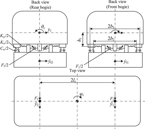
Since the control purpose of this paper is to suppress the lateral vibration of the car body, a simplified model of the lateral vibration of the car body is developed with reference to the research of Zong et al. [14], which is used to ensure the accuracy of the model and facilitate the subsequent controller design. Ignoring the influence of bogie yaw and roll motion on car body, the motion equation of lateral, yaw and roll of car body is as follows.

Car body lateral motion: (18) $\begin{array}{rl}& M_{\text{c}}{\ddot{y}}_c+K_{\text{s}y}(y_c+l{\psi }_c-h_1{\theta }_c-y_{\text{t}1})\\ & +C_{\text{s}y}({\dot{y}}_c+l{\dot{\psi }}_c-h_1{\dot{\theta }}_c-{\dot{y}}_{\text{t}1})\\ & +K_{\text{s}y}(y_c-l{\psi }_c-h_1{\theta }_c-y_{\text{t}2})\\ & +C_{\text{s}y}({\dot{y}}_c-l{\dot{\psi }}_c-h_1{\dot{\theta }}_c-{\dot{y}}_{\text{t}2})=(F_1+F_2)\end{array}$(18) Car body yaw motion: (19) $\begin{array}{rl}& J_{\text{c}z}{\ddot{\psi }}_c+K_{\text{s}y}l(y_c+l{\psi }_c-h_1{\theta }_c-y_{\text{t}1})\\ & +C_{\text{s}y}l({\dot{y}}_c+l{\dot{\psi }}_c-h_1{\dot{\theta }}_c-{\dot{y}}_{\text{t}1})\\ & -K_{\text{s}y}l(y_c-l{\psi }_c-h_1{\theta }_c-y_{\text{t}2})\\ & -C_{\text{s}y}l({\dot{y}}_c-l{\dot{\psi }}_c-h_1{\dot{\theta }}_c-{\dot{y}}_{\text{t}2})=l(F_1-F_2)\end{array}$(19)

Car body roll motion: (20) $\begin{array}{rl}& J_{\text{c}x}{\ddot{\theta }}_c-K_{\text{s}y}{h}_1(y_c+l{\psi }_c-h_1{\theta }_c-y_{\text{t}1})\\ & -C_{\text{s}y}{h}_2({\dot{y}}_c+l{\dot{\psi }}_c-h_1{\dot{\theta }}_c-{\dot{y}}_{\text{t}1})\\ & -K_{\text{s}y}{h}_1(y_c-l{\psi }_c-h_1{\theta }_c-y_{\text{t}2})\\ & -C_{\text{s}y}{h}_2({\dot{y}}_c-l{\dot{\psi }}_c-h_1{\dot{\theta }}_c-{\dot{y}}_{\text{t}2})\\ & +2K_{\text{s}y}{b}_2^2{\theta }_c+2C_{\text{s}y}{b}_3^2{\dot{\theta }}_c=-h_2(F_1+F_2)\end{array}$(20) The lateral vibration of car body is the coupled result of lateral, yaw and roll motion in practice. In this paper, two measuring points located on the bottom of car body are selected to measure the lateral vibration of car body, which displacements are y₁ and y₂ respectively, and the relationship between y_c, ψ_c and θ_c and y₁, y₂ is as follows: (21) $y_1=y_{\text{c}}+l_{\text{c}}{\psi }_{\text{c}}+h_{\text{c}}{\theta }_{\text{c}},y_2=y_{\text{c}}-l_{\text{c}}{\psi }_{\text{c}}+h_{\text{c}}{\theta }_{\text{c}}$(21) By regarding the lateral motion velocity of the front and rear bogies $\dot{y}$_t1 and $\dot{y}$_t2 as external excitations, the control forces F₁ and F₂ generated by the MR damper as control force inputs, and the lateral acceleration of the car body $\ddot{y}$₁ and $\ddot{y}$₂ as the measurement outputs, a 3-DOF simplified model of car body lateral vibration (simplified model) is developed (Figure 3).

Figure 3. Simplified model of car body lateral vibration.

The state space equation describing the simplified model is presented in (22) based on Equations (18)–(20). (22) $\begin{array}{rl}\dot{x}& =Ax+B_{1}w+B_{2}u\\ y& =Cx+D_{1}w+D_{2}u\end{array}$(22) To facilitate writing, define the following variables: y_Yc= (y₁–y₂)/2, y_Yt= (y_t1–y_t2)/2, Δy_Y= (y_Yc–y_Yt)/2, y_Lc= (y₁+ y₂)/2, y_Lt= (y_t1+ y_t2)/2, Δy_L= (y_Lc–y_Lt)/2. And the specific form of x, y, w, u, A, B₁, C, D₁ and D₂ is as follows:

$\begin{array}{rl}x& =[\begin{array}{cccccc}{\dot{y}}_{\text{Yc}}& \mathrm{\Delta }{y}_{\text{Y}}& {\dot{y}}_{\text{c}}& \mathrm{\Delta }{y}_{\text{L}}& {\dot{\theta }}_{\text{c}}& {\theta }_{\text{c}}\end{array}{]}^{\text{T}},w=[\begin{array}{cc}{\dot{y}}_{\text{t}1}& {\dot{y}}_{\text{t2}}\end{array}{]}^{\text{T}},u=[\begin{array}{cc}{F}_1& F_2\end{array}{]}^{\text{T}},y=[\begin{array}{cc}{\ddot{y}}_1& {\ddot{y}}_{\text{2}}\end{array}{]}^{\text{T}}\\ A& =\left[\begin{array}{cccccc}-2C_{\text{s}y}{l_{\text{c}}}^2\text{/}{J}_{\text{c}z}& -2K_{\text{s}y}{l_{\text{c}}}^2\text{/}{J}_{\text{c}z}& 0& 0& 0& 0\\ 1& 0& 0& 0& 0& 0\\ 0& 0& -2C_{\text{s}y}\text{/}{M}_c& -2K_{\text{s}y}\text{/}{M}_c& 2C_{\text{s}y}{h}_2\text{/}{M}_c& 2K_{\text{s}y}{h}_1\text{/}{M}_c\\ 0& 0& 1& 0& 0& 0\\ 0& 0& 2C_{\text{s}y}{h}_2\text{/}{J}_{cx}& 2K_{\text{s}y}{h}_1\text{/}{J}_{\text{c}x}& -2(C_{\text{s}y}{h}_2^2+C_{\text{s}y}{b}_3^2)\text{/}{J}_{\text{c}x}& -2(K_{\text{s}y}{h}_1^2+K_{\text{s}y}{b}_2^2)\text{/}{J}_{\text{c}x}\\ 0& 0& 0& 0& 1& 0\end{array}\right]\\ B_1& =\left[\begin{array}{cc}{C}_{\text{s}y}{l}_{\text{c}}^2\text{/}{J}_{\text{c}z}& -C_{\text{s}y}{l}^2\text{/}{J}_{\text{c}z}\\ -1\text{/}2& 1\text{/}2\\ C_{\text{s}y}\text{/}{M}_c& C_{\text{s}y}\text{/}{M}_c\\ -1\text{/}2& -1\text{/}2\\ C_{\text{s}y}{h}_2\text{/}{J}_{\text{c}x}& C_{\text{s}y}{h}_2\text{/}{J}_{\text{c}x}\\ 0& 0\end{array}\right],B_2=\left[\begin{array}{cc}{l}_{\text{c}}^2\text{/}2J_{\text{c}z}& -l_{\text{c}}^2\text{/}2J_{\text{c}z}\\ 0& 0\\ 1\text{/}{M}_c& 1\text{/}{M}_c\\ 0& 0\\ -h_2\text{/}{J}_{\text{c}x}& -h_2\text{/}{J}_{\text{c}x}\\ 0& 0\end{array}\right]\end{array}$ $\begin{array}{rl}C& =[\begin{array}{cccc}-2C_{\text{s}y}{l}_{\text{c}}^2\text{/}{J}_{\text{c}z}& -2K_{\text{s}y}{l}_{\text{c}}^2\text{/}{J}_{\text{c}z}& -2C_{\text{s}y}(1\text{/}{M}_c-h_{\text{c}}{h}_2\text{/}{J}_{\text{c}x})& -2K_{\text{s}y}(1\text{/}{M}_c-h_{\text{c}}{h}_1\text{/}{J}_{\text{c}x})\\ 2C_{\text{s}y}{l}_{\text{c}}^2\text{/}{J}_{\text{c}z}& 2K_{\text{s}y}{l}_{\text{c}}^2\text{/}{J}_{cz}& -2C_{\text{s}y}(1\text{/}{M}_c-h_{\text{c}}{h}_2\text{/}{J}_{\text{c}x})& -2K_{\text{s}y}(1\text{/}{M}_c-h_{\text{c}}{h}_1\text{/}{J}_{\text{c}x})\end{array}\\ & \begin{array}{cc}2C_{\text{s}y}[h_2\text{/}{M}_c-h_{\text{c}}(b_3^2\text{ + }{h}_2^2\left)\text{/}{J}_{\text{c}x}\right]& 2K_{\text{s}y}[h_1\text{/}{M}_c-h_{\text{c}}(b_2^2\text{ + }{h}_1^2\left)\text{/}{J}_{\text{c}x}\right]\\ 2C_{\text{s}y}[h_2\text{/}{M}_c-h_{\text{c}}(b_3^2\text{ + }{h}_2^2\left)\text{/}{J}_{\text{c}x}\right]& 2K_{\text{s}y}[h_1\text{/}{M}_c-h_{\text{c}}(b_2^2\text{ + }{h}_1^2\left)\text{/}{J}_{\text{c}x}\right]\end{array}]\\ D_1& =\left[\begin{array}{cc}{C}_{\text{s}y}\text{(}1\text{/}{M}_c-h_c{h}_2\text{/}{J}_{\text{c}x})+C_{\text{s}y}{l}_{\text{c}}^2\text{/}{J}_{\text{c}z}& C_{\text{s}y}\text{(}1\text{/}{M}_c-h_{\text{c}}{h}_2\text{/}{J}_{\text{c}x})-C_{\text{s}y}{l}_{\text{c}}^2\text{/}{J}_{\text{c}z}\\ C_{\text{s}y}\text{(}1\text{/}{M}_c-h_c{h}_2\text{/}{J}_{\text{c}x})-C_{\text{s}y}{l}_{\text{c}}^2\text{/}{J}_{\text{c}z}& C_{\text{s}y}\text{(}1\text{/}{M}_c-h_{\text{c}}{h}_2\text{/}{J}_{\text{c}x})+C_{\text{s}y}{l}_{\text{c}}^2\text{/}{J}_{\text{c}z}\end{array}\right],\\ D_2& =\left[\begin{array}{cc}1\text{/}{M}_c+l_{\text{c}}^2\text{/}2J_{\text{c}z}-h_{\text{c}}{h}_2\text{/}{J}_{\text{c}x}& 1/M_c-l_{\text{c}}^2\text{/}{J}_{\text{c}z}-h_{\text{c}}{h}_2\text{/}{J}_{\text{c}x}\\ 1\text{/}{M}_c-l_{\text{c}}^2\text{/}2J_{\text{c}z}-h_{\text{c}}{h}_2\text{/}{J}_{\text{c}x}& 1/M_c+l_{\text{c}}^2\text{/}2J_{\text{c}z}-h_{\text{c}}{h}_2\text{/}{J}_{\text{c}x}\end{array}\right]\end{array}$

4.3. Robust controller design

The following is the design of the robust controller, the core of the control system, whose function is to calculate the desired control force according to the vibration signal measured by the sensor. In this paper, a robust controller is built based on the simplified model, which is designed by the μ-synthesis method considering the effect of time delay.

The lateral vibration of the car body includes yaw and rolling pendulum motion (the coupling of lateral and roll motion), so the controller is divided into yaw controller and rolling pendulum controller. According to the simplified model, state space models describing the yaw and rolling pendulum motion of car body are presented as follows:

Yaw motion model of car body: (23) $\begin{array}{rl}{\dot{x}}_{\text{Y}}& =A_{\text{Y}}{x}_{\text{Y}}+{B_1}_{\text{Y}}{w}_{\text{Y}}+{B_2}_{\text{Y}}{u}_{\text{Y}}\\ y_{\text{Y}}& =C_{\text{Y}}{x}_{\text{Y}}+{D_1}_{\text{Y}}{w}_{\text{Y}}+D_{2\text{Y}}{u}_{\text{Y}}\end{array}$(23) where $\begin{array}{rl}{x}_{\text{Y}}& =[{\begin{array}{cc}{\dot{y}}_{\text{Yc}}& \mathrm{\Delta }{y}_{\text{Y}}]\end{array}}^{\text{T}},w_{\text{Y}}={\dot{y}}_{\text{Yt}},\\ u_{\text{Y}}& =(F_1-F_2)/2,y_{\text{Y}}={\ddot{y}}_{\text{Yc}}\\ A_{\text{Y}}& =\left[\begin{array}{cc}-2C_{\text{s}y}{l}^2/J_{cz}& -2K_{\text{s}y}{l}^2/J_{cz}\\ 1& 0\end{array}\right],\\ {B_1}_{\text{Y}}& =\left[\begin{array}{c}2C_{\text{s}y}{l}^2/J_{cz}\\ -1\end{array}\right],{B_2}_{\text{Y}}=\left[\begin{array}{c}{l}^2/J_{cz}\\ 0\end{array}\right]\\ C_{\text{Y}}& =\left[\begin{array}{cc}-2C_{\text{s}y}{l}^2/J_{cz}& -2K_{\text{s}y}{l}^2/J_{cz}\end{array}\right],\\ {D_1}_{\text{Y}}& =\left[\begin{array}{c}2C_{\text{s}y}{l}^2/J_{cz}\end{array}\right],{D_2}_{\text{Y}}=\left[\begin{array}{c}{l}^2/J_{cz}\end{array}\right]\end{array}$Rolling pendulum motion model of car body: (24) $\begin{array}{rl}{\dot{x}}_{\text{L}}& =A_{\text{L}}{x}_{\text{L}}+{B_1}_{\text{L}}{w}_{\text{L}}+{B_2}_{\text{L}}{u}_{\text{L}}\\ y_{\text{L}}& =C_{\text{L}}{x}_{\text{L}}+{D_1}_{\text{L}}{w}_{\text{L}}+D_{2\text{L}}{u}_{\text{L}}\end{array}$(24) where $\begin{array}{rl}{x}_{\text{L}}& =[\begin{array}{cccc}{\dot{y}}_{\text{c}}& \mathrm{\Delta }{y}_{\text{L}}& {\dot{\theta }}_{\text{c}}& {\theta }_{\text{c}}\end{array}{]}^{\text{T}},w_{\text{L}}={\dot{y}}_{\text{Lt}},\\ u_{\text{L}}& =(F_1+F_2)\text{/}2,y_{\text{L}}={\ddot{y}}_{\text{Lc}}\\ A_{\text{L}}& =[\begin{array}{ccc}-2C_{\text{s}y}\text{/}{M}_c& -2K_{\text{s}y}\text{/}{M}_c& 2C_{\text{s}y}{h}_2\text{/}{M}_c\\ 1& 0& 0\\ 2C_{\text{s}y}{h}_2\text{/}{J}_{\text{c}x}& 2K_{\text{s}y}{h}_1\text{/}{J}_{\text{c}x}& -2(C_{\text{s}y}{h}_2^2+C_{\text{s}y}{b}_3^2)\text{/}{J}_{\text{c}x}\\ 0& 0& 1\end{array}\\ & \begin{array}{c}2K_{\text{s}y}{h}_2\text{/}{M}_c\\ 0\\ -2(K_{\text{s}y}{h}_1^2+K_{\text{s}y}{b}_2^2)\text{/}{J}_{\text{c}x}\\ 0\end{array}],\\ {B_1}_{\text{L}}& =\left[\begin{array}{c}2C_{\text{s}y}\text{/}{M}_c\\ -1\\ -2C_{\text{s}y}{h}_2\text{/}{J}_{\text{c}x}\\ 0\end{array}\right],{B_2}_{\text{L}}=\left[\begin{array}{c}2\text{/}{M}_c\\ 0\\ -2h_2\text{/}{J}_{\text{c}x}\\ 0\end{array}\right]\\ C_{\text{L}}& =[2C_{sy}(-1\text{/}{M}_c+h_{\text{c}}{h}_2\text{/}{J}_{\text{c}x})2K_{sy}(-1\text{/}{M}_c+h_{\text{c}}{h}_1\text{/}{J}_{\text{c}x})\\ & 2C_{sy}[h_2\text{/}{M}_c-h_{\text{c}}(h_2^2+b_3^2\left)\text{/}{J}_{\text{c}x}\right]\\ & 2K_{sy}[h_2/M_c-h_{\text{c}}(h_1^2+b_2^2)\text{/}{J}_{\text{c}x}\left]\right]\\ {D_1}_{\text{L}}& =\left[\begin{array}{c}2C_{\text{s}y}(1\text{/}{M}_c-h_{\text{c}}{h}_2\text{/}{J}_{\text{c}x})\end{array}\right],\\ {D_2}_{\text{L}}& =\left[\begin{array}{c}2\text{/}{M}_c-2h_{\text{c}}{h}_2\text{/}{J}_{\text{c}x}\end{array}\right]\end{array}$The yaw and rolling pendulum motion model takes u_Y and u_L as the control force input, takes y_Y and y_L as the measurement output. y_Y and y_L can be obtained by measuring the acceleration of the car body $\ddot{y}$₁ and $\ddot{y}$₂. u_Y and u_L are the control forces calculated by the controller, which can be converted into F₁ and F₂.

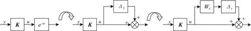
Figure 4. Closed loop control system of car body lateral vibration with time delay: (a) closed loop control system for yaw motion and (b) closed loop control system for rolling pendulum motion.

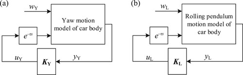
Assuming that the control force output by the controller can be fully tracked, a car body lateral vibration closed-loop control system with time delay in input channel is developed, on which the yaw motion controller K_Y and rolling pendulum motion controller K_L are designed based (Figure 4).

To design the robust controller, the time delay e^−τs in the input channel is transformed into the model perturbation Δ_τ of the control system in this paper and the process is shown in Figure 6.

First, let Δ₁=  e^−τs–1, e^−τs decomposes into parallel connection of Δ₁ and 1. According to the robust control theory, the following requirements need to be met: when τ > 0, ||Δ₁||_∞ < 1, so further conversion is required.

Then draw amplitude frequency curve of Δ₁ in different τ and fit the upper bound W_c so that |W_c|>|Δ₁| is established in all frequency ranges, which is shown in (25). And the comparison of W_c and Δ₁ in different τ is shown in Figure 5. (25) $W_c=\frac{2.2s}{s+10}$(25) Finally, normalize Δ_1, let Δ_τ= Δ₁W_c⁻¹, ||Δ_τ||_∞<1, so that time delay e^−τs is transformed into model perturbation Δ_τ (Figure 6).

Figure 5. Amplitude curve of W_c and Δ₁ with different τ.

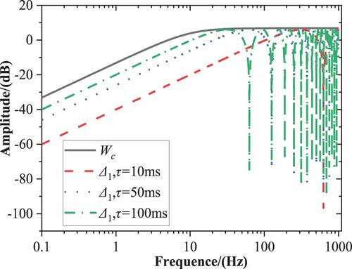
Figure 6. Schematic of the progress turning time delay into model perturbation.

According to the performance requirements of the controller, specify the controlled output. First, the controller needs to suppress the lateral vibration of the car body, which is mainly concentrated in the low-frequency range within 0.5–10 Hz, so the lateral vibration outputs y_Y and y_L are weighted through the band-stop filter W_y to obtain the controlled outputs z_yY and z_yL. Meanwhile, the control force controller should be concentrated in the low-frequency range as much as possible, so the control forces u_Y and u_L are weighted through the high-pass filter W_u to obtain the controlled outputs z_uY and z_uL. Finally, the design structure of the robust controller for yaw and rolling pendulum motion is shown in Figure 7. (26) $W_y=\frac{s^2+1.17s+25}{s^2+15.54s+25},W_u=\frac{s+50}{s+500}$(26) The “musyn” function in the robust controller toolbox of Matlab® is used to calculate the controllers K_Y and K_L respectively. The final controller is integrated by K_Y and K_L which takes $\ddot{y}$₁ and $\ddot{y}$₂ as input and F₁ and F₂ as output. $\ddot{y}$₁ and $\ddot{y}$₂ are measured by the sensor, then y_Y and y_L are obtained after operation 1 shown in (27). u_Y and u_L are obtained according to y_Y and y_L, which are further transformed into desired control forces F₁ and F₂ after operation 2 shown in (28). Considering the contribution of yaw and rolling pendulum motion to the lateral vibration of car body and comparing the results of a series of weight values, select w_L= 8 and w_Y= 1. 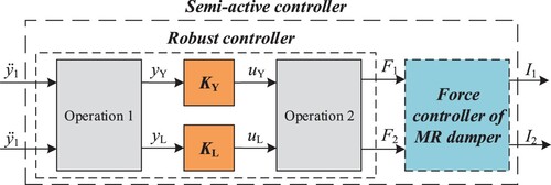(27) $\text{Operation 1: }{y}_{\text{Y}}=\frac{{\ddot{y}}_1-{\ddot{y}}_2}{2},y_L=\frac{{\ddot{y}}_1+{\ddot{y}}_2}{2}$(27) (28) $\begin{array}{rl}\text{Operation }2:F_{\text{1}}& =\frac{w_{\text{L}}{u}_{\text{L}}+w_{\text{Y}}{u}_{\text{Y}}}{2},\\ F_2& =\frac{w_{\text{L}}{u}_{\text{L}}-w_{\text{Y}}{u}_{\text{Y}}}{2}\end{array}$(28) Finally, the robust controller and the force controller form the semi-active controller (Figure 8).

Figure 7. Design structure of robust controller: (a) robust controller for yaw motion and (b) robust controller for rolling pendulum motion.

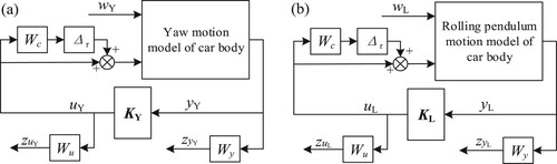
Figure 8. Schematic of the semi-active controller.

4.4. Predictive compensator design

4.4.1. Smith predictive compensation model

To reduce the effect of time delay, this paper adopts Smith predictive compensation control method [32], whose schematic is shown in Figure 9. Where G_c(s) represents the transfer function of the controller, G_p(s) and Ĝ_p(s) represent the actual and estimated transfer function of the controlled object, τ represents time delay.

Figure 9. Schematic of Smith predictive compensation control.

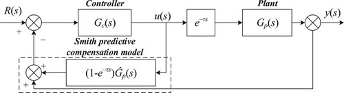
The transfer functions of the close-loop system with and without Smith predictive compensation model are described as (29) and (30). It can be found that the denominator of the transfer function will not contain e^(−τs) after Smith predictive compensation model is added if both the estimated transfer function of the controlled object and estimated value of time delay are accurate (Ĝ_p(s) = G_p(s)), which means the effect of time delay is eliminated. (29) $\frac{Y\left(s\right)}{R\left(s\right)}=\frac{G_c\left(s\right)G_p\left(s\right)}{1+G_c\left(s\right)G_p\left(s\right)e^{(-\tau s)}}$(29) (30) $\frac{Y\left(s\right)}{R\left(s\right)}=\frac{G_c\left(s\right)G_p\left(s\right)e^{(-\tau s)}}{1+G_c\left(s\right){\hat{G}}_p\left(s\right)+G_c\left(s\right)e^{(-\tau s)}\left(G_p\right(s)-{\hat{G}}_p(s\left)\right)}$(30) However, it’s difficult to obtain accurate model describing dynamic system of HSTs and the track irregularity is difficult to measure using sensors directly in practice. Therefore, it’s not practicable to directly use Smith predictive compensation method to reduce the effect of time delay.

The actual controlled object is the whole model of HSTs in this paper, but the purpose is supressing the lateral vibration of car body. Therefore, regarding the simplified model as an approximation of the whole model of HSTs, the Smith predictive compensation method of MR semi-active suspension system is proposed (Figure 10).

Figure 10. Schematic of MR semi-active suspension system with Smith predictive compensation model.

The Smith predictive compensation model includes the simplified model and force calculator, takes the command current I₁ and I₂, the relative velocity of front and rear MR damper $\dot{y}$_d1 and $\dot{y}$_d2, and lateral velocity of front and rear bogie $\dot{y}$_t1 and $\dot{y}$_t2 as input and takes the predictive value of lateral acceleration of front and rear ends of car body $\ddot{y}$_p1 and $\ddot{y}$_p2 as output. I₁ and I₂ are calculated by semi-active controller, $\dot{y}$_d1, $\dot{y}$_d2, $\dot{y}$_t1 and $\dot{y}$_t2 can be measured by sensors. The Smith predictive compensation model is an approximation of the actual model of HST to predict $\ddot{y}$₁ and $\ddot{y}$₂ to reduce the effect of time delay.

4.4.2. Lateral velocity predictor

$\ddot{y}$₁ and $\ddot{y}$₂ depend on I₁, I₂ and $\dot{y}$_d1, $\dot{y}$_d2, $\dot{y}$_t1 and $\dot{y}$_t2 for the simplified model, among which I₁ and I₂ are obtained through the semi-active controller and not delayed. Therefore, to obtain more accurate $\ddot{y}$_p1 and $\ddot{y}$_p2, it’s necessary to design predictor to predict $\dot{y}$_d1, $\dot{y}$_d2, $\dot{y}$_t1 and $\dot{y}$_t2, which is called lateral velocity predictor in this paper.

The transfer function of predictor is G_v(s), whose amplitude frequency characteristics and phase frequency characteristics meet (31) ideally, where τ is the prediction length, φ is the leading angle, and ω is the frequency of the input signal. (31) $|G_v\left(j\omega \right)|=1,\frac{\phi }{360f}=\tau$(31) The ideal predictor is not possible to realize, but possible to approach in a certain frequency range. In this paper, a predictor is designed to predict $\dot{y}$_d1, $\dot{y}$_d2, $\dot{y}$_t1 and $\dot{y}$_t2 based on the phase-lead compensator that is often used in the research of time delay problems [33–35].

As shown in (32), the transfer function describing the lateral velocity predictor can be regarded as the combination of two phase-lead compensators and one proportional amplification link, where the parameters a_v and T_v determine the characteristics of the predictor. In (33), φ_m is the maximum lead angle, ω_m is corresponding frequency of φ_m, and |G_c(ω_m)| = 1. The predictor can advance the phase of the signal by about φ_m near ω_m with the amplitude not too distorted. (32) $G_v\left(s\right)=\frac{1}{a_v}\frac{{(a_v{T}_{v}s+1)}^2}{{(T_{v}s+1)}^2}$(32) (33) ${\phi }_m=2\arcsin \frac{1-a_v}{1+a_v},{\omega }_m=\frac{1}{\sqrt{a_v}T}$(33) If the frequency component of the signal is concentrated near f_m and prediction length is τ, then ω_m= 2πf_m and φ_m= 360f_mτ, parameters a_v and T_v can be obtained through (33). 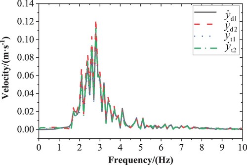(34) $a_v=\frac{1+\sin \left({\phi }_m/2\right)}{1-\sin \left({\phi }_m/2\right)},T_v=\frac{1}{{\omega }_m}\sqrt{\frac{1-\sin \left({\phi }_m/2\right)}{1+\sin \left({\phi }_m/2\right)}}$(34) $\dot{y}$_d1, $\dot{y}$_d2, $\dot{y}$_t1 and $\dot{y}$_t2 are collectively referred to as the lateral velocity in this paper. The frequency domain analysis of the lateral velocity is carried out to find out its main frequency components, before designing the predictor. Figure 11 shows the amplitude frequency curve of $\dot{y}$_d1, $\dot{y}$_d2, $\dot{y}$_t1 and $\dot{y}$_t2 when passive control is adopted and it can be found that the frequency component concentrated mainly in the range of 2–4 Hz, and the main frequency is about 2.8 Hz.

Figure 11. Amplitude frequency curve of the lateral velocity.

The amplitude frequency curve of the lateral velocity is related to the level of excitation, running speed, and it's also the reflection of the vibration mode. The vibration model mainly depends on the parameters related to mass and stiffness in the suspension, which will not change during semi-active control. Meanwhile, this paper assumes that the level of excitation is constant and the running speed is 300 km/h. Therefore, it should be similar to Figure 11 when the semi-active control is applied.

In summary, the characteristics of the lateral velocity in frequency domain include concentrated in low frequency, and stable under certain working conditions. Therefore, the predictor proposed above can be used to predict it.

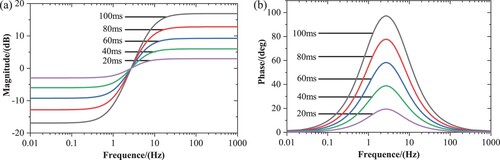
The predictor is designed with f_m= 2.8 Hz and ω_m = 5.6π rad/s, then φ_m= 504τ and the design parameters a_v and T_v can be obtained according to (34). It can be found that a_v and T_v are only related to τ. Therefore, when τ is known, the predictor can be obtained directly through (35). Figure 12 is the frequency characteristic curve of the predictor with different τ. (35) $a_v=\frac{1+\sin \left(504\tau \right)}{1-\sin \left(504\tau \right)},T_v=\frac{1}{5.6\pi }\sqrt{\frac{1-\sin \left(504\tau \right)}{1+\sin \left(504\tau \right)}}$(35) It can be seen that the magnification is about 0 and the lead angle is about 504τ near 2.8 Hz, which meets the requirements; In the range of 0–2.8 Hz, the phase can be approximately advanced, but the magnification will be reduced. In the range of more than 2.8 Hz, the leading effect of phase is poor, and the magnification of high-frequency components in the signal is amplified, which means the performance of predictor on high-frequency vibration is very poor. In practical, it is necessary to add a low-pass filter in front of the predictor to limit its high-frequency response.

Figure 12. Frequency characteristic curve of the predictor with different time delay: (a) amplitude frequency curve and (b) phase frequency curve.

Apply the proposed predictor to predict $\dot{y}$_d1, $\dot{y}$_d2, $\dot{y}$_t1 and $\dot{y}$_t2 in different τ when passive control is adopted respectively. The accuracy of prediction is evaluated through the prediction error e_p, shown in (36), where v_a represents the actual values of $\dot{y}$_d1, $\dot{y}$_d2, $\dot{y}$_t1 and $\dot{y}$_t2, and v_p represents their corresponding predicted values. (36) $e_p=\sqrt{\frac{1}{T}{\int }_0^T{(v_a-v_p)}^2\text{d}t}$(36) The results of e_p are shown in Table 4. It can be found that e_p increases with τ, which indicates that the accuracy of prediction decreases with τ, but still remains in an acceptable range when τ = 100 ms, so the designed predictor can be used to predict the lateral velocity. Meanwhile, to show the accuracy of prediction clearly, the comparison between predicted value and the actual value when τ = 50 ms is shown in Figure 13.

Figure 13. Validation of the lateral velocity predictor when τ = 50 ms: (a) $\dot{y}$_d1; (b) $\dot{y}$_d2; (c) $\dot{y}$_t1; (d) $\dot{y}$_t2.

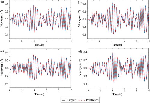
Table 4. Errors of the lateral velocity predictor with different τ.

τ(ms) ep(m·s^−1)	10	20	30	40	50	60	70	80	90	100
${\dot{y}}_{d1}$	0.008	0.016	0.023	0.029	0.035	0.041	0.047	0.053	0.058	0.063
${\dot{y}}_{d2}$	0.008	0.016	0.023	0.030	0.037	0.043	0.049	0.055	0.060	0.066
${\dot{y}}_{t1}$	0.008	0.015	0.021	0.028	0.033	0.039	0.045	0.050	0.055	0.060
${\dot{y}}_{t2}$	0.008	0.015	0.022	0.029	0.035	0.040	0.046	0.051	0.057	0.062

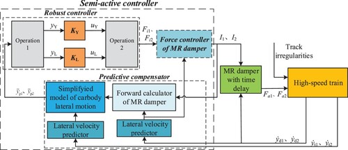
4.5. Robust predictive compensation control system for MR semi-active suspension

According to the study above, the control strategy consists of three parts: robust controller that calculates the desired control force of the front and rear ends of the car body, force controller that calculates the command current according to the control force and the motion velocity of MR damper, and the predictive compensator that predicts the lateral velocity including $\dot{y}$_d1, $\dot{y}$_d2, $\dot{y}$_t1 and $\dot{y}$_t2.

The final semi-active control system is shown in Figure 14. Collecting the relative velocity of the front and rear MR dampers $\dot{y}$_d1 and $\dot{y}$_d2, the lateral motion velocity of the front and rear bogies $\dot{y}$_t1 and $\dot{y}$_t2, and the command current I₁ and I₂ as the input of the predictive compensator to calculate $\ddot{y}$_p1 and $\ddot{y}$_p2, and the robust controller calculates the desired control force of front and rear ends of the car body F_i1 and F_i2 through $\ddot{y}$_p1 and $\ddot{y}$_p2, then command currents I₁ and I₂ are obtained through the force controller. After the MR damper receives I₁ and I₂, the actual control forces F_a1 and F_a2 generated suppress the lateral vibration of the car body.

Figure 14. Schematic of robust predictive compensation control system for MR semi-active suspension with time delay.

5. Simulation results

For brevity, the semi-active controller designed in this paper is denoted as controller 1. To invalidate the effectiveness of the proposed control strategy, several controllers are designed for comparing and analysing. It is noted that these controllers use the same force controller. Because the lateral vibration of car body of different vehicle models is relatively similar, only one vehicle model is adopted. Its parameters are presented in Appendix A.

The robust controller considering the effect of time delay is designed in 4.3, and the semi-active controller composed of it and the force controller is denoted as controller 2. Compared with controller 1, controller 2 does not contain predictive compensator. And a conventional robust controller is designed, not considering the effect of time delay, which is similar to that of controller 2 and does not include W_c and Δ_τ in the structure of controller design, and the semi-active controller formed by its combination with the force controller is denoted as controller 3. Finally, according to the SH-ADD control strategy [21,36], an active controller is designed, which consists of two parts to generate the control forces F₁ and F₂ respectively, and the specific mathematical form is as follows: (37) $\begin{array}{rl}{F}_1& =\{\begin{array}{l}{C}_{max}{\dot{y}}_{\text{d}1},\left[\right({\ddot{y}}_1^2-{{\alpha }_1}^2{\dot{y}}_1^2\le 0),y_1{\dot{y}}_{\text{d}1}\ge 0]\\ \text{ or }\text{[}({\ddot{y}}_1^2-{{\alpha }_1}^2{\dot{y}}_1^2>0),y_1{\dot{y}}_{\text{d}1}\ge 0\\ C_{min}{\dot{y}}_{\text{d}1},\text{otherwise}\end{array}\text{]},\\ F_2& =\{\begin{array}{l}{C}_{max}{\dot{y}}_{\text{d}2},\left[\right({\ddot{y}}_2^2-{{\alpha }_2}^2{\dot{y}}_2^2\le 0),y_2{\dot{y}}_{\text{d2}}\ge 0]\\ \text{ or }\text{[}({\ddot{y}}_2^2-{{\alpha }_2}^2{\dot{y}}_2^2>0),y_2{\dot{y}}_{\text{d2}}\ge 0]\\ C_{min}{\dot{y}}_{\text{d}2},\text{otherwise}\end{array}\end{array}$(37) where C_max and C_min represent the maximum and minimum damping coefficients of the damper. Considering the MR damper used in this paper, C_max= 40 kN/m·s⁻¹, C_min= 7 kN/m·s⁻¹ are taken here. α₁ and α₂ is the conversion coefficient, which is obtained here through the (38), where ${\overline{\ddot{y}}}_1$ and ${\overline{\ddot{y}}}_2$ are the root mean square values within the last 10 s. For convenience, it is replaced by the root mean square value within 10 s when passive control is adopted, and then α₁ and α₂ are determined in advance. The semi-active controller composed of SH-ADD active controller and the inverse model is denoted as controller 4. (38) ${\alpha }_1=-614{\overline{\ddot{y}}}_1+55.74,{\alpha }_2=-614{\overline{\ddot{y}}}_2+55.74$(38) The control performance of each controller is evaluated by simulation compared with the passive control, which keeps the lateral damping of secondary suspension at 25 kN/m·s⁻¹. The “Bogacki–Shampine” solver is adopted for the simulation, the step size is fixed at 1e–3s, and the total simulation time is 25 s.

When time delay is 50 and 100 ms, the time-domain curves (8–10 s) of car body acceleration with different controllers adopted are shown in Figures 15 and 16, RMS values of car body acceleration and lateral ride index [37] are listed in Table 5. It can be found that controller 1 can always suppress the lateral vibration of the car body, and the control performance of controller 2 is weaker than that of controller 1, but better than that of controllers 3 and 4, which indicates that controller 1 has strong robustness to time delay, followed by controller 2, and controllers 3 and 4 are the worst, which do not consider the effect of time delay in their design.

Figure 15. Time histories of the car body accelerations with different controller adopted when τ = 50 ms: (a) lateral accelerations, (b) yaw accelerations and (c) roll accelerations.

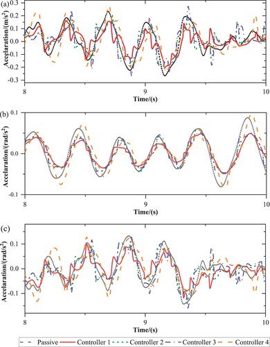
Figure 16. Time histories of the car body accelerations with different controllers adopted when τ = 100ms: (a) lateral accelerations, (b) yaw accelerations and (c) roll accelerations.

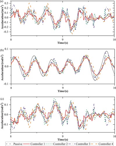
Table 5. RMS values of car body accelerations and lateral ride index with different controller adopted when τ = 50, 100 ms.

			τ = 50 ms				τ = 100 ms
			Controller				Controller
		Passive	1	2	3	4	1	2	3	4
RMS values	${\ddot{y}}_c$ (m/s^2)	0.136	0.080	0.090	0.092	0.101	0.094	0.127	0.128	0.121
	${\ddot{\psi }}_c$ (rad/s^2)	0.036	0.023	0.024	0.024	0.024	0.024	0.029	0.031	0.028
	${\ddot{\theta }}_c$ (rad/s^2)	0.072	0.044	0.048	0.048	0.051	0.052	0.067	0.066	0.064
Lateral ride index	Front	2.496	2.151	2.222	2.261	2.388	2.165	2.267	2.339	2.259
	Rear	2.503	2.169	2.327	2.331	2.390	2.197	2.328	2.324	2.260

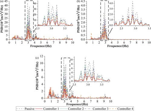
Figures 17 and 18 show PSDs of car body acceleration with different controllers adopted when the time delay is 50 and 100 ms. It can be found that the car body lateral vibration is mainly concentrated in the range of 0.5–10 Hz, and the vibration around 1 and 3 Hz is strong. Controller 1 can still suppress the lateral vibration of the car body better around 3 Hz well, while the vibration around 3 Hz is significantly strengthened when other controllers are adopted.

Figure 17. PSDs of the car body accelerations with different controller adopted when τ = 50 ms: (a) lateral accelerations, (b) yaw accelerations and (c) roll accelerations.

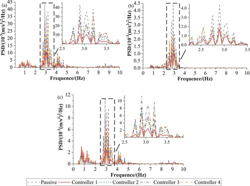
Figure 18. PSDs of the car body accelerations with different controllers adopted when τ = 100 ms: (a) lateral accelerations, (b) yaw accelerations and (c) roll accelerations.

To further validate robustness to time delay of controller 1, Figures 19 and 20 show the RMS values of car body acceleration and lateral ride index with different controllers adopted when the time delay increases from 0 to 100 ms.

Figure 19. RMS values of car body accelerations with different controllers adopted: (a) lateral accelerations, (b) yaw accelerations and (c) roll accelerations.

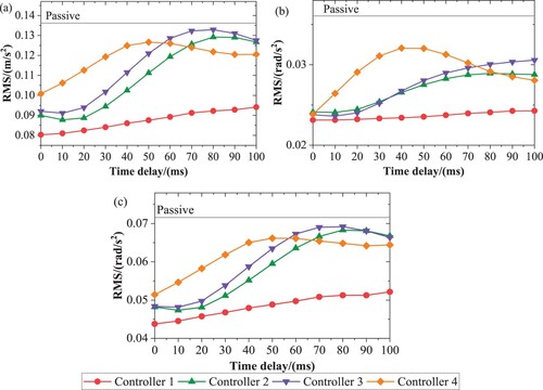
Figure 20. Lateral ride index with different controller adopted: (a) lateral accelerations, (b) yaw accelerations and (c) roll accelerations.

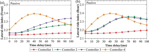
For controller 1, the increase of RMS values and lateral ride index with time delay is the slowest. Even when time delay is 100 ms, better control performance can still be achieved. The performance of controllers 2 and 3 is close, but that of controller 2 is slightly stronger. The robustness to time delay of controller 4 is the worst, whose performance will degrade obviously when the delay is small and increase first and then decrease with the increase of delay. Meanwhile, the difference between controllers 1 and 2 is only whether there is a predictive compensator, the comparison of their results can prove that the predictive compensator can effectively reduce the effect of time delay.

To sum up, the semi-active controller proposed in this paper has strong robustness to time delay and can maintain good control performance when time delay of MR semi-active suspension in the range of 0–100 ms.

6. Conclusion and discussion

Aiming at the time delay problem of MR semi-active suspension of HSTs, this paper proposes a control strategy with strong robustness to time delay, including the force controller of MR damper, robust controller and predictive compensator. The effectiveness of the control strategy is validated by simulation. Some conclusions are summarized as follows.

1. Each controller can maintain good performance without time delay, but the performance of conventional controller will be significantly reduced with the increase of time delay, even worse than passive control.

2. The control strategy proposed in this paper can maintain good performance when time delay is no more than 100 ms, which indicates it has strong robustness to time delay.

3. The comparison of the controller with and without predictive compensator shows that the predictive compensator proposed in this paper can significantly reduce the effect of time delay.

On the other hand, this paper only considers the vibration control of vehicles and ignores the interaction between vehicles, track and railway. Currently, some experts have studied the vehicle–track–bridge dynamic interaction and proposed the vehicle–track–bridge dynamic interaction model [38], which is a structural system consisting of a high-speed railway bridge and a high-speed train. Meanwhile, the tuned mass dampers (TMDs), including multiple tuned mass dampers (MTMDs), series tuned mass dampers (STMDs) and so on, have been adopted for vibration control of railway bridges [39–42]. Based on that, the problem of applying semi-active control to TMDs and the vibration control of a structural system composed of vehicle, track and bridge need to be explored in depth.

Disclosure statement

No potential conflict of interest was reported by the author(s).

Additional information

Funding

This work was supported by the National Natural Science Foundation of China [grant number U2034210], the National Natural Science Foundation of China [grant number 51975487] and the National Natural Science Foundation of China [grant number 52372402].

Appendices

Appendix A.

Vehicle model parameters

Table A1. Parameter values and definitions of the 17-DOF model.

Parameter	Value	Unit	Meaning description
Mc	32,000	kg	Mass of car body
Jcz	2.24 × 10^6	kg·m^2	Yaw moment of inertia of car body
Jcx	75,000	kg·m^2	Roll moment of inertia of car body
Mt	3296	kg	Mass of bogie frame
Jtz	2100	kg·m^2	Yaw moment of inertia of bogie frame
Jtx	1900	kg·m^2	Roll moment of inertia of bogie frame
Mw	1750	kg	Mass of wheelset
Jwz	1400	kg·m^2	Yaw moment of inertia of wheelset
Ksx	1.7 × 10^5	N/m	Secondary longitudinal stiffness
Ksy	1.75 × 10^5	N/m	Secondary lateral stiffness
Ksz	3.4 × 10^5	N/m	Secondary vertical stiffness
Csx	2.5 × 10^5	N·s/m	Secondary longitudinal damping
Csy	2.5 × 10^4	N·s/m	Secondary lateral damping
Csz	8 × 10^4	N·s/m	Secondary vertical damping
Kpx	1.45 × 10^7	N/m	Primary longitudinal stiffness
Kpy	7.5 × 10^6	N/m	Primary lateral stiffness
Kpz	6.65 × 10^5	N/m	Primary vertical stiffness
Cpz	1.5 × 10^4	N·s/m	Primary vertical damping
h1	0.77	m	Vertical distance from car body centre of gravity to secondary spring
h2	0.77	m	Vertical distance from car body centre of gravity to secondary lateral damper
h3	0.2175	m	Vertical distance from bogie frame centre of gravity to secondary spring
h4	−0.2085	m	Vertical distance from bogie frame centre of gravity to primary suspension
h5	0.2175	m	Vertical distance from bogie frame centre of gravity to secondary lateral damper
hc	0.5	m	Vertical distance from car body centre of gravity to car body bottom
lc	9	m	Half of bogie centre pin spacing
l1	1.25	m	Half of wheelbase
b	0.7465	m	Half of wheelset contact distance
b1	1	m	Half of primary suspension spacing (lateral)
b2	1	m	Half of secondary spring spacing (lateral)
b3	1	m	Half of secondary vertical damper spacing (lateral)
r0	0.4575	m	Wheel rolling radius
λ	0.05		Effective wheel conicity
f11	1.12 × 10^7		Longitudinal creep coefficient
f22	9.98 × 10^6		Lateral creep coefficient
Ωc	0.8426	rad/m	Truncated wavenumber
Ωr	0.0206	rad/m	Truncated wavenumber
Ωc	0.4380	rad/m	Truncated wavenumber
Aa	2.119 × 10^−7		Scalar factor of lateral alignment
Av	4.032 × 10^−7		Scalar factor of cross-level

Appendix B.

Verification of the dynamic model of HSTs

Table B1. Comparison of time domain results at different speed.

		V = 100 km/h	V = 200 km/h	V = 300 km/h
Lateral acceleration RMS value (m/s^2)	Ref. [43]	0.064	0.1389	0.1933
	This paper	0.054	0.1335	0.2197
Yaw acceleration RMS value (rad/s^2)	Ref. [43]	0.0231	0.035	0.0413
	This paper	0.0162	0.031	0.0556
Roll acceleration RMS value (rad/s^2)	Ref. [43]	0.0275	0.0606	0.0843
	This paper	0.0246	0.0557	0.0897
Lateral acceleration peak-peak value (m/s^2)	Ref. [14]	\	\	1.0743
	This paper	\	\	1.1613
Yaw acceleration peak-peak value (rad/s^2)	Ref. [14]	\	\	0.2915
	This paper	\	\	0.3533
Roll acceleration peak-peak value (rad/s^2)	Ref. [14]	\	\	0.4342
	This paper	\	\	0.4941

Figure B1. Comparison of PSDs of car body lateral acceleration: (a) ref. [12], (b) model in this paper.

Figure B2. Comparison of PSDs of car body yaw acceleration: (a) ref. [12], (b) model in this paper.

Figure B3. Comparison of PSDs of car body roll acceleration: (a) ref. [12], (b) model in this paper (“Passive-on”: the command current of MR damper is maximum, “Passive-off”: the command current of MR damper is minimum, and the speed is 200 km/h, the track irregularities is from the German high-speed high disturbance).

Figure C1. The change of damping force when the command current raises from 0.5 A to 1 A [17] (RD-1005-3 MR damper).

Appendix C.

Relevant supporting material of the time delay discussed in this paper

Table C1. Response time under different system compliance [17] (RD-1005-3 MR damper).

System compliance	No rubber	Single rubber	Double rubber
Response time (ms)	27.9	51.78	68.60