
 ?Mathematical formulae have been encoded as MathML and are displayed in this HTML version using MathJax in order to improve their display. Uncheck the box to turn MathJax off. This feature requires Javascript. Click on a formula to zoom.
Abstract
The principal contribution of this paper is the feedback design of an output trajectory tracking controller applied to a certain class of mechanical systems. The controller does not need velocity measurements for its implementation and achieves the trajectory tracking control aim. We propose adaptive estimators to determine the plant parameters and constant external perturbations. When the plant is affected by time-variant external perturbations, an observer filter that can be implemented to recover an estimation of the time-variant perturbations can replace the adaptive estimator. The closed-loop stability is analysed throughout Lyapunov tools. We illustrate the performance of the proposed control structure via numerical simulations and experiments, the numerical simulations are carried out for a pendulum coupled to a DC motor and the experiments are accomplished for a mass-spring-damper system.
1. Introduction
Most mechanical systems need velocity measurement for feedback to solve the tracking control problem. If a velocity sensor is not available for feedback, it can be used as a velocity observer or a differentiator [Citation1–5].
We can find in the literature previous works about tracking control in mechanical systems without velocity measurements. In [Citation6], a simple robust control law is given to solve the tracking problem without using velocity observers, which improves the tracking accuracy in soft bending actuators. They consider lumped system uncertainties that are compensated using a discontinuous term within the control law. In [Citation7], a solution to the problem of formation consensus control of second-order nonholonomic systems is proposed. They use output feedback considering that the forward and angular velocities are not available for measurement, and in the stability analysis they prove uniform global asymptotic stability for the closed-loop system, which guarantees robustness regarding bounded disturbances. Another example, in [Citation8] a controller that obviates the need for state observers to solve the tracking control problem of induction motors by using energy shaping (passivity-based) design techniques is proposed. In [Citation9], an output feedback controller is proposed to solve the trajectory tracking problem in finite time without using observers. This scheme was proposed for robot manipulators having actuators that exhibit torque saturation. In [Citation10], a state feedback finite-time stabilizing algorithm is developed, and the proposed synthesis is based on the disturbance compensation, relying on the dirty differentiation and sliding mode approach. We can find other works about tracking control that obviates the need for a velocity observer using the dirty differentiation in [Citation11–14]. In [Citation15], an output feedback adaptive robust controller (ARC) scheme based on discontinuous projection method has been developed for high-performance robust motion control of linear motors. The proposed controllers consider the effect of model uncertainties coming from the inertia load, friction force, force ripple and bounded external disturbances, although the controller renders good performance, it cannot identify the plant parameters and disturbances separately, also velocity estimation is required as feedback. More recently, in [Citation16] also an adaptive optimal controller is proposed to solve the tracking control problem of model-free nonlinear systems where a dynamic neural network identifier is developed to identify the unknown dynamics . In this approach, all the states must be available to be used as feedback. Our work, as the papers aforementioned, does not need velocity measurements for feedback, but the significant difference between our work regarding the previous ones is that no observer, filter or differentiator is needed to achieve asymptotic closed-loop stability, and it is enough to have access to position measurements to achieve the control aim considering all the plant parameters as known and zero perturbations. In the scenario when the plant parameters are unknown and also the system is affected by exogenous perturbations, we propose adaptive estimators that, by using position measurements purely, they can estimate the plant parameters independently as well as the constant external perturbation.
Velocity observer-based controller design should consider that the observer is formed from the software control loops and it may cause the system to be unstable under certain conditions [Citation17], which may cause potential security risks when applied to any mechanical system.
Therefore, a robust controller without using velocity from observers, but with only position information, is a preferred solution for applications [Citation18–20]. This paper proposes a novel robust tracking controller for a class of mechanical systems with unknown parameters and external perturbations. The main contributions are summarized as follows:
The design of a tracking controller for a class of second-order systems may be applied not only to mechanical systems but to electronic, hydraulic, pneumatic, among other systems as well. The proposed controller does not need velocity measurements for feedback to achieve the tracking control aim, and it only needs position measurements. The proposed solution to the tracking problem does not use any observer, differentiator or filter to achieve the control aim when there are no external perturbations or the external perturbation is a constant. When there are time-variant external perturbations, we use indirectly an observer to recover an estimation of the external perturbation, but we do not use the velocity estimation as feedback to the controller.
In the design and stability analysis of adaptive estimators, these estimators solely need position measurements as feedback to give us an approximation of the plant parameters and, in case there is the constant external perturbation.
The stability analysis is based on Lyapunov's theory, which guarantees the stability of the closed-loop system. The dynamic controller only has one tunable gain parameter, making it simple to tune, there just needs to meet the conditions given by the Lyapunov stability analysis.
Thus the core contribution of this work relays on the proposed control structure and its stability proof; some features of the controller are the identification of the plant parameters and disturbances separately and the lack of necessity of velocity measurements for feedback.
We structure the rest of this paper according to the following sections: in Section 2, the statement of the problem is described for second-order dynamical systems, which encompasses mechanical systems of 1 degree of freedom that may include the actuator dynamics within. In Section 3, the general structure of the controller is proposed. The stability proof of the closed-loop system using Lyapunov tools [Citation21,Citation22] is presented in Section 4. In Section 5, adaptive estimator designs are presented to recover plant parameters and constant external perturbations which are fully unknown, and its stability proofs guarantee boundedness of the solutions. In Section 6, an alternative is presented that can be applied when the closed-loop system is affected by time-variant perturbations. This approach is based on a discontinuous observer where the high-frequency component can be filtered after reaching the nominal stage by a Butterworth filter (presented in Section 6.1) to recover the time-variant perturbations. In Section 7, numerical simulations and experiments are performed using the proposed control structure for time-variant perturbations in a pendulum with DC motor and in a mass-spring-damper system. Section 8 includes a conclusion and future work.
2. Problem statement
The problem addressed in the paper is the tracking control of a class of mechanical systems, through the design and implementation of a continuous robust control without using velocity measurements.
The following state–space equations govern the dynamics of the class of mechanical systems considered in this paper:
(1)
(1) although this type of system has been addressed previously [Citation23–26], several dynamic systems fit into this structure (Equation3
(3)
(3) ) such as mechanical, thermal, electronic, electrical, hydraulic, pneumatic systems among others. The states are
and
, the functions
and
are nonlinear,
is also an invertible function, the parameters a, and
are positive constants that are considered totally unknown,
describes the effect of external unmeasurable perturbations, y stands for the output of the system.
The proposed control structure for this type of systems is
(2)
(2) where τ is the proposed algorithm, the rest of the terms are well known and we use them for compensation. Substituting (Equation2
(2)
(2) ) into (Equation1
(1)
(1) ), the closed-loop system stands as follows:
(3)
(3)
3. Control design
The controller is based on a proportional control plus compensation terms which are got using an uncertainty and disturbance estimator. We consider that most of the plant parameters are unknown, as well as external perturbations. For system (Equation3(3)
(3) ), the following control design is proposed:
(4)
(4) where u is the proposed algorithm,
is a gain parameter, the desired trajectory
is at least
and the error stands as
. The parameters
,
are estimations of the plant parameters,
is the estimation of the external perturbation. We can note that this control algorithm (Equation4
(4)
(4) ) does not need
measurements or estimation to solve the trajectory tracking problem, as it is going to be proven in the stability section. Substituting (Equation4
(4)
(4) ) in (Equation3
(3)
(3) ) and rewriting the remaining system in function of the errors:
(5)
(5) where
and
, where
is the desired trajectory assumed to be twice differentiable. The estimation errors are given by
,
and
.
Note that closed-loop system (Equation5(5)
(5) ) has only one equilibrium point (when the estimation errors
,
,
are zero) given by
(6)
(6) otherwise, it becomes an equilibria set.
4. Stability proof
Theorem 4.1
Consider the perturbed system (Equation1(1)
(1) ) under the control law (Equation2
(2)
(2) ) and (Equation4
(4)
(4) ), then the error dynamics
and
of the closed-loop system (Equation5
(5)
(5) ) converge to the equilibria asymptotically while the estimation errors
,
and
remain bounded.
Proof.
For this purpose, let us propose the following Lyapunov candidate function: (7)
(7) which it is a positive definite function by keeping
with
,
,
and
. Based strictly on design purposes, let us propose
(8)
(8) The derivative of (Equation7
(7)
(7) ) along the trajectories of (Equation5
(5)
(5) ) and (Equation8
(8)
(8) ) is given by
(9)
(9) note that
is a negative semi-definite function while
. We can conclude the following by fulfilling the conditions imposed by (Equation7
(7)
(7) ) and (Equation9
(9)
(9) ), the
and
, meanwhile the states
,
and
remain bounded. Thus the closed-loop stability proof is completed.
5. Adaptive estimator design
This section should design an adaptive algorithm to estimate the plant parameters a and b, as well as the external perturbation w, to achieve it let us assume a, b and w are constants, therefore the following expressions are valid:
(10)
(10) Given that we do not have access to
measurements, let us take (Equation8
(8)
(8) ) and integrate them by parts,
(11)
(11) Considering (Equation10
(10)
(10) ) and (Equation11
(11)
(11) ), we can get the adaptive estimators for the plant parameters and external perturbation
(12)
(12) The stability proof of (Equation12
(12)
(12) ) was presented in the previous section.
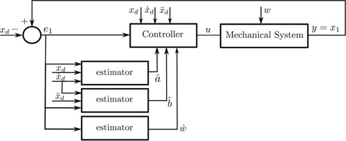
Figure shows the proposed control structure to solve the tracking problem in a class of mechanical systems without velocity measurement, considering full estimation of plant parameters and estimation of a constant external perturbation.
Figure 1. The proposed control structure considers completely unknown plant parameters and a constant external perturbation, also unknown.
6. Estimation of time-variant perturbations
This section explains how to estimate w when it is variable through time. It is assumed that w is bounded by an upper bound, so it satisfies . The estimation includes uncertainties, disturbances and non-well modelled parameters. This estimation is made indirectly using a discontinuous velocity observer for the system (Equation3
(3)
(3) ), although the velocity estimation given by the observer is not used implicitly in the controller design (Equation4
(4)
(4) ) its discontinuous term is used to get the estimation of w. The following observer design is based on the previous works of [Citation27,Citation28]. The proposed discontinuous observer has the form
(13)
(13) the variables
and
stand for the errors; likewise, the gain parameters are
,
and
. Now let us rewrite (Equation13
(13)
(13) ) in terms of the observed errors
(14)
(14) The main concern of the present discontinuous observer is the stability analysis of (Equation14
(14)
(14) ). Strictly for stability purposes, we are going to make a change of variables
and
, the dynamics of the system (Equation14
(14)
(14) ) according to the new state–space representation stand as follows:
(15)
(15) Note that, if we can prove
and
as time goes to infinity, then indirectly
and
will also tend to zero as time increases. The stability proof of (Equation15
(15)
(15) ) is given in [Citation29], where one condition to satisfy is the fulfilment of
.
6.1. Filter
According to [Citation30], the equivalent output injection or equivalent control coincides with the slow component of the discontinuous term in (Equation13
(13)
(13) ) when the state is on the discontinuity surface (this is
). The equivalent control provides information about unmeasured dynamics such as uncertainties, disturbances and non-well modelled parameters those contained in w. By this way, throughout using a low-pass filter the equivalent control can be recovered, keeping in mind an adequate cut-off frequency selection, for further details [Citation31,Citation32]. Given this background, any topology of low-pass filters, such as Bessel, Butterworth, Chebyshev, elliptic and so on, can be implemented; in this case, we are going to use a second-order (although the order may vary) low-pass Butterworth filter to estimate (online) the equivalent control
as follows:
(16)
(16) where
is the cut-off frequency of the filter. Here, the filter input is the discontinuous term of the observer,
. By denoting the output of the filter as
, and choosing a cut-off frequency
that minimizes the phase-delay, it is possible to assume
(17)
(17) where
is the estimation of the perturbation, and the supremum of the estimation error
for
.
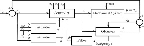
Figure shows the proposed control structure to solve the tracking problem in a class of mechanical systems without velocity measurement, considering full estimation of plant parameters and estimation of time-variant external perturbations.
Figure 2. The proposed control structure considers completely unknown plant parameters and time-variant external perturbations which are not completely known.
7. Numerical simulations
7.1. Pendulum with DC motor
Another system that fits in the class of mechanical systems addressed by this paper is the pendulum, which includes a DC motor as an actuator. The dynamic model of the DC motor can be represented by a second-order linear differential equation, which relates the voltage input υ applied to the motor armature, to the output torque τ delivered by the motor. An sketch of DC motor with negligible armature inductance is shown in Figure , where the pendular device is in red colour. A simplified linear dynamic model of the DC motor (without the pendulum) is given by
(18)
(18) where
: rotor inertia [kg·m
τ: net applied torque after the set of gears at the load axis [N·m],
r: gear reduction ratio (in general
υ: armature voltage [V],
Figure 3. Pendular device with a DC motor.
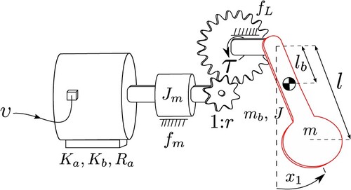
Therefore, (Equation18(18)
(18) ) describes the motion of the DC motor coupled mechanically through a set of gears, where the input is the voltage υ applied to the armature of the motor, and the output is the torque τ applied to the load.
The equation of motion of a pendular arm under the action of gravity (see Figure , pendular arm in red colour) is given by
(19)
(19) where
m: load mass at the tip of the arm (assumed to be punctual);
l: distance from the rotating axis to the load m;
g: gravity acceleration;
τ: applied torque at the rotating axis;
Equation (Equation19(19)
(19) ) may also be written in the compact form
(20)
(20) where
Hence, the complete dynamic model of the pendular device may be obtained by substituting τ from the model of the DC motor (Equation18
(18)
(18) ) into the dynamics of the pendular arm (Equation20
(20)
(20) ),
(21)
(21) To carry out the closed-loop simulation, we have taken the initial conditions, plant parameters and controller gains as shown in Table .
Table 1. Simulation parameters.
The numerical simulation results of the pendular system (Equation21(21)
(21) ) under the control law (Equation4
(4)
(4) ), using the parameter estimator (Equation12
(12)
(12) ), and disturbance estimator (Equation16
(16)
(16) ) were performed using Matlab code.
Now let us make a performance comparison of the controllers. We will use a first-order sliding mode controller [Citation4] and a PD control plus compensation terms, named PD+ in [Citation33]. As output just is measured, to estimate
the observer presented in (Equation13
(13)
(13) ) has been considered (keep in mind that the controller proposed in this work does not need access to
). The external perturbation
and the parameter
are unknown, making it more difficult to achieve the zero error in the trajectory tracking.
The sliding mode control algorithm tested is as follows:
(22)
(22) using
, and the sliding surface
with
and
, where
is the output of the observer (Equation13
(13)
(13) ).
The PD+ algorithm considered is as follows:
(23)
(23) where
(1/ms
) and
(1/ms
); the variable
is as well taken from the observer.
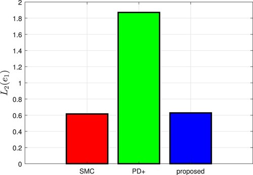
The performance index of each controller is going to be got using the norm defined as
(24)
(24) where T represents the simulation time. The best controller performance index corresponds to the smaller
norm. A high-performance index represents poor controller performance.
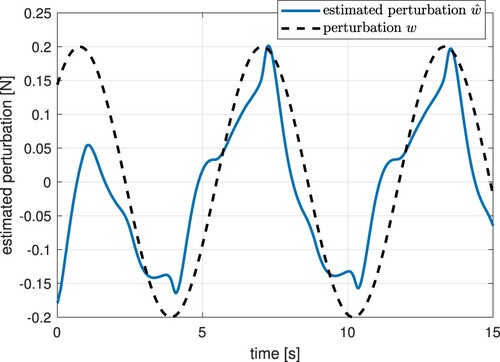
In Figure , the tracking reference (black dashed line) and the trajectory tracking of the three controllers can be viewed. Figure shows the derivative of the tracking reference (black dashed line) and the velocity. In Figure , the phase portraits are presented, where using the proposed controller we can appreciate a slope because of the effect caused by the transient stage of the parameter and disturbance estimators in the closed-loop system. We presented the position and velocity errors in Figures and , correspondingly. The continuous control signal of the proposed control given in volts units appears in Figure , which includes the estimation of a group of parameters and perturbations within it. Figure considers the estimation of a group of plant parameters. In Figure , we can observe that after 4 seconds, almost the discontinuity surface of the observer is reached, and the estimated perturbation can be recovered after completing the Butterworth filter. Figure shows the energy signal when applied different controllers to the closed-loop system. Figure shows the comparative results using the
index, where the proposed controller renders good agreement compared with other controllers.
Figure 4. Trajectory tracking of (black dashed line) (simulation).
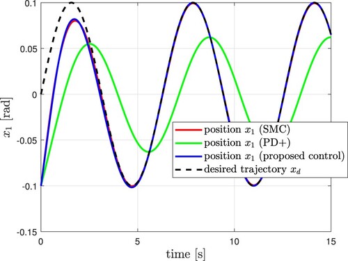
Figure 5. Derivative of trajectory tracking of (black dashed line) (simulation).
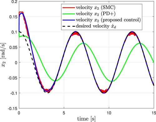
Figure 6. Phase portrait (simulation).
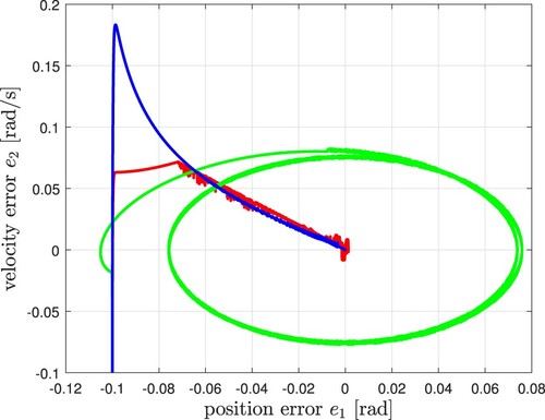
Figure 7. Tracking error (simulation).
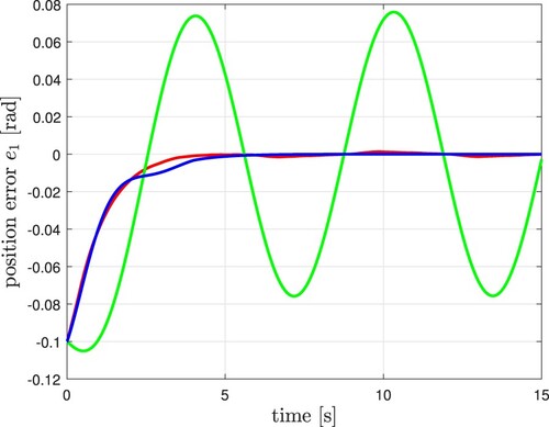
Figure 8. Velocity error (simulation).
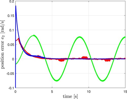
Figure 9. Control signal (simulation).
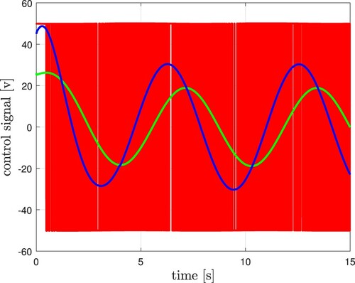
Figure 10. Estimation of damping coefficient (simulation).
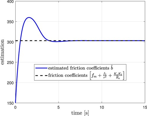
Figure 11. Estimated perturbation (simulation).
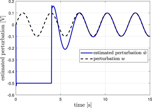
Figure 12. Energy signal (simulation).
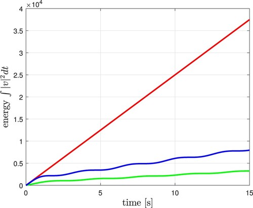
Figure 13. Performance index (simulation).
8. Experiments
8.1. Mass-spring-damper system
The proposed control structure (Equation4(4)
(4) ), (Equation12
(12)
(12) ), (Equation13
(13)
(13) ), and filter (Equation16
(16)
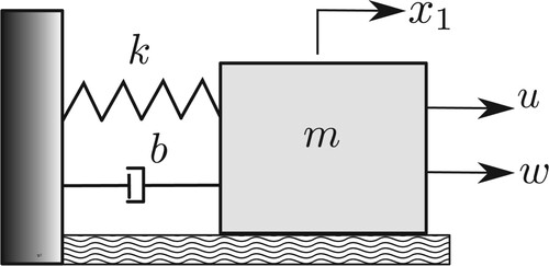
(16) ) is tested through experiments in a mass-spring-damper system from ECP (educational control products) model 210: rectilinear plant, as shown in Figure and depicted in Figure , whose equations are given by
(25)
(25) where
is the mass,
is the spring stiffness,
stands for the damping coefficient,
is the motor force constant and
represents the effect of the uncertainties and external unmeasurable disturbances.
Figure 14. Mass-spring-damper system comprises model 210: rectilinear plant from educational control products (ECP) and data acquisition board MicroLabBox from dSPACE.
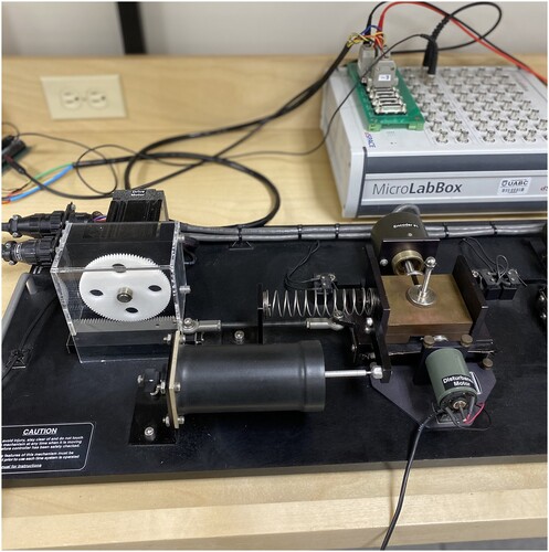
Figure 15. Outline of the mass-spring-damper system.
The initial conditions, plant parameters and controller gains used are given in Table .
Table 2. Experimental parameters.
The experimental results were performed using Matlab. In Figure , the tracking reference (black dashed line) and the trajectory tracking can be seen. It can be appreciated the position error in Figure . The continuous control signal appears in Figure , which includes the estimation of parameters and perturbations within it. Figures and illustrate the estimation of plant parameters. Figure shows the disturbance estimation.
Figure 16. Trajectory tracking of (black dashed line) (experiment).
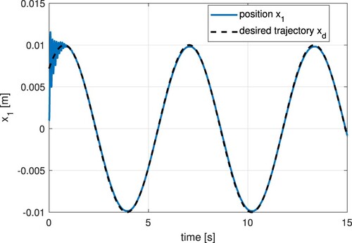
Figure 17. Tracking error (experiment).
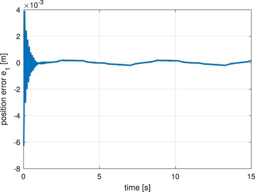
Figure 18. Control signal (experiment).
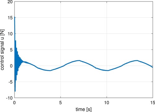
Figure 19. Estimation of spring stiffness (experiment).
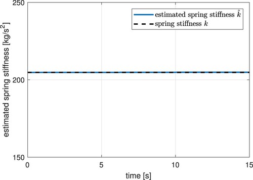
Figure 20. Estimation of damping coefficient (experiment).
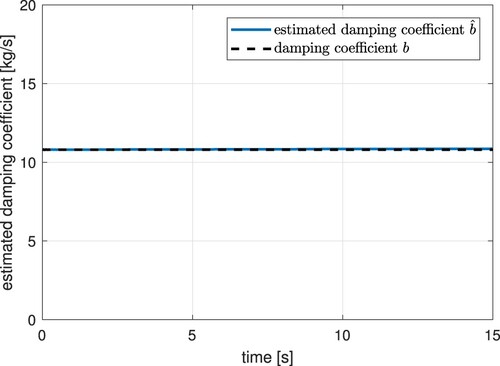
Figure 21. Estimated perturbation (experiment).
9. Conclusion
According to the results presented in this paper, we can assure that velocity measurements are not needed to achieve the tracking control aim in a certain class of mechanical systems; even sometimes, it is unnecessary to design and apply an observer or a filter to estimate the velocity; it is enough to just have position measurements available for feedback to achieve the control objective.
The adaptive estimators proposed in this paper can estimate the parameter of the plant separately, using only position measurements as feedback to achieve the task. Therefore, most of the plant parameters are not required to be previously identified to apply the controller.
In the scenario when external perturbations are affecting the plant, two proposals emerge: the first one is the design of an adaptive estimator created to estimate constant external perturbations. The second proposal is the design of a discontinuous observer, where the time-variant external perturbation can be estimated by filtering the high-frequency component of the observer by a low-pass filter, we chose a second-order Butterworth filter to accomplish the task.
There are offered stability proofs using Lyapunov tools for the two control structures proposed. To highlight the theoretical results, there were carried out closed-loop simulations and experiments in a pendulum with a DC motor and in a mass-spring-damper system, respectively.
To the best of our knowledge, the problem solved in this work has not been addressed formerly in the literature, thus some future research efforts will be conducted to enhance the results presented here.
Disclosure statement
No potential conflict of interest was reported by the author(s).
References
- Romero JG, Moreno JA, Aguilar ÁAM. An adaptive speed observer for a class of nonlinear mechanical systems: theory and experiments. Automatica. 2021;130:109710. doi:10.1016/j.automatica.2021.109710
- Arteaga MA, Gutiérrez-Giles A, Pliego-Jiménez J. Velocity observer design. In: Local stability and ultimate boundedness in the control of robot manipulators. Springer; 2022. p. 143–164.
- Rosas D, Alvarez J, Rosas P, et al. Robust observer for a class of nonlinear SISO dynamical systems. Math Problem Eng. 2016;2016:Article ID 6182143. doi:10.1155/2016/6182143
- Shtessel Y, Edwards C, Fridman L, et al. Sliding mode control and observation. New York: Springer; 2014.
- Rascon R, Rosas D, Hernandez-Fuentes I, et al. Robust tracking control for mechanical systems using only position measurements. ISA Trans. 2020;100:299–307. doi:10.1016/j.isatra.2019.12.012
- Cao G, Huo B, Yang L, et al. Model-based robust tracking control without observers for soft bending actuators. IEEE Robot Autom Lett. 2021;6(3):5175–5182. doi:10.1109/LRA.2021.3071952
- Loria A, Nuno E, Panteley E. Observerless output-feedback consensus-based formation control of 2nd-order nonholonomic systems. IEEE Trans Automat Control. 2021;67:6934–6939.
- Espinosa G, Ortega R. State observers are unnecessary for induction motor control. Syst Control Lett. 1994;23(5):315–323. doi:10.1016/0167-6911(94)90063-9
- Cruz-Zavala E, Nuno E, Moreno JA. Trajectory-tracking in finite-time for robot manipulators with bounded torques via output-feedback. Int J Control. 2021;94(4):1–15.
- Furtat I, Orlov Y, Fradkov A. Finite-time sliding mode stabilization using dirty differentiation and disturbance compensation. Int J Robust Nonlinear Control. 2019;29(3):793–809. doi:10.1002/rnc.v29.3
- Loría A. Observers are unnecessary for output-feedback control of lagrangian systems. IEEE Trans Automat Control. 2016 Apr;61(4):905–920. doi:10.1109/TAC.2015.2446831
- Sira-Ramírez H, Zurita-Bustamante EW, Huang C. Equivalence among flat filters, dirty derivative-based PID controllers, ADRC, and integral reconstructor-based sliding mode control. IEEE Trans Control Syst Technol. 2019;28(5):1696–1710. doi:10.1109/TCST.87
- Zavala-Río A, Zamora-Gómez GI, Sanchez T, et al. Output-feedback finite-time and exponential tracking continuous control for mechanical systems with constrained inputs. Int J Robust Nonlinear Control. 2022;32(3):1393–1424. doi:10.1002/rnc.v32.3
- Marchi M, Fraile L, Tabuada P. Dirty derivatives for output feedback stabilization; 2022. arXiv:220201941, preprint.
- Xu L, Yao B. Output feedback adaptive robust precision motion control of linear motors. Automatica. 2001;37(7):1029–1039. doi:10.1016/S0005-1098(01)00052-8
- Yin Y, Fu Z, Lu Y. Online adaptive optimal tracking control for model-free nonlinear systems via a dynamic neural network. Automatika. 2023;64(3):431–440. doi:10.1080/00051144.2023.2170058
- Ellis G. Observers in control systems: a practical guide. San Diego, CA: Elsevier; 2002.
- Shao K, Zheng J, Wang H, et al. Recursive sliding mode control with adaptive disturbance observer for a linear motor positioner. Mech Syst Signal Process. 2021;146:107014. doi:10.1016/j.ymssp.2020.107014
- Dirksz DA, Scherpen JM. On tracking control of rigid-joint robots with only position measurements. IEEE Trans Control Syst Technol. 2012;21(4):1510–1513. doi:10.1109/TCST.2012.2204886
- Rascón R, Moreno-Valenzuela J. Output feedback controller for trajectory tracking of robot manipulators without velocity measurements nor observers. IET Control Theory Appl. 2020;14(14):1819–1827. doi:10.1049/cth2.v14.14
- Pérez-Alcocer R, Moreno-Valenzuela J. A novel Lyapunov-based trajectory tracking controller for a quadrotor: experimental analysis by using two motion tasks. Mechatronics. 2019;61:58–68. doi:10.1016/j.mechatronics.2019.05.006
- De Queiroz MS, Dawson DM, Nagarkatti SP, et al. Lyapunov-based control of mechanical systems. New York: Springer Science & Business Media; 2012.
- Choi SB, Park DW, Jayasuriya S. A time-varying sliding surface for fast and robust tracking control of second-order uncertain systems. Automatica. 1994;30(5):899–904. doi:10.1016/0005-1098(94)90180-5
- Bartolini G, Ferrara A, Usai E. Output tracking control of uncertain nonlinear second-order systems. Automatica. 1997;33(12):2203–2212. doi:10.1016/S0005-1098(97)00147-7
- Park KB, Tsuji T. Terminal sliding mode control of second-order nonlinear uncertain systems. Int J Robust Nonlinear Control. 1999;9(11):769–780. doi:10.1002/(ISSN)1099-1239
- Tian GT, Duan GR. Robust model reference control for uncertain second-order system subject to parameter uncertainties. Trans Inst Meas Control. 2022;44(1):88–104. doi:10.1177/0142331220904544
- Rosas Almeida DI, Alvarez J, Fridman L. Robust observation and identification of nDOF Lagrangian systems. Int J Robust Nonlinear Control. 2007;17(9):842–861. doi:10.1002/(ISSN)1099-1239
- Orlov Y, Aoustin Y, Chevallereau C. Finite time stabilization of a perturbed double integrator – Part I: continuous sliding mode-based output feedback synthesis. IEEE Trans Autom Control. 2011;56(3):614–618. doi:10.1109/TAC.2010.2090708
- Rascón R. Robust tracking control for a class of uncertain mechanical systems. Automatika. 2019;60(2):124–134. doi:10.1080/00051144.2019.1584693
- Utkin VI. Sliding modes in control and optimization. Berlin: Springer-Verlag; 1992.
- Drakunov S. An adaptive quasioptimal filter with discontinuous parameters. Avtomat Telemekh. 1983; (9):76–86.
- Shtessel Y, Edwards C, Fridman L, et al. Sliding mode control and observation. Springer New York; 2014.
- Kelly R, Davila VS, Perez JAL. Control of robot manipulators in joint space. Leipzig, Germany: Springer Science & Business Media; 2006.