The Computational Singular Perturbation/Perfectly Stirred Reactor Approach in Reduced Chemistry of Premixed Ethanol Combustion

Abstract

Ethanol is a bio-fuel widely used in engines as a fuel or fuel additive. It is, in particular, attractive because it can be easily produced in high quality from renewable resources. Its properties are of interest in many fields, such as gas turbines applications as well as fuel cells. In the past decades, research in chemistry and engineering has put a lot of effort into a better understanding of its gas-phase chemical kinetic properties during combustion processes. This work describes a methodology to define an optimal expression of the reaction progress variable in the context of tabulated chemistry in laminar premixed combustion. The choice of the reaction progress variable is based on the investigation of the wide range of consumption rates of the species involved in the reaction. Two methods are used: the computational singular perturbation method and a sensitivity analysis of the time scales evaluated with a perfectly stirred reactor. The thermochemical databases computed with these techniques are compared in the cases of a freely propagating flame and a Bunsen flame, in the laminar premixed regime and under stoichiometric conditions. The influence of the chemical kinetics on the laminar flame speed is estimated from the results of the freely propagating flame. The case where the differences in the performance between the databases become more pronounced is the Bunsen flame, where some databases lead to a premature ignition prediction of the flame.

KEYWORDS:

• Chemical time scales
• Laminar premixed flames
• Reaction progress variable
• Reduced chemistry
• Steady state species

Introduction

In the past few decades, industry and research in the combustion field have faced the challenge to improve the combustion systems in order to address the necessity to decrease emissions of pollutants. An essential strategy to respond to the environment issues was to include non-fossil fuels in the primary energy source; this action opened the way to the investigation of the performance of several alternative fuels, for example, the bioalchohols (ethanol, methanol, and butanol). The interest for these cleaner fuels has directed the aim of the research to a better understanding of the fundamentals of their chemical kinetics. Yalamanchili et al. (2005) proposed a chemical kinetic mechanism to predict and investigate the combustion process of methanol; work from Black et al. (2010) and Dagaut et al. (2009) gave an insight on the oxidation of butanol. Only a few complex kinetic mechanisms have been proposed for ethanol combustion, for example, Norton and Dryer (1992) and Marinov (1999). One of the advantages of using such fuels is their blending properties, as studied by Dagaut and Togbé (2012). Both experimental (Egolfopoulos et al., 1992) and numerical studies play a major role in this process, but numerical analysis is especially attractive for the relatively low cost. However, when detailed chemistry is used, the larger the size of the kinetic mechanism, the higher the computational cost. Numerical simulations of flames might even be prohibitive if mechanisms with hundreds of species and reactions are taken into account. This applies specifically for turbulent combustion. To address the problem of the computational cost, the necessity of reduced kinetic mechanisms arises, as well as the need to decrease the number of degrees of freedom of the reaction phenomena; thus, the importance of kinetic mechanisms with a minimum number of species and reactions involved, and a new numerical strategy that does not solve for all the species but only for a reduced number of representative variables.

In this article, in particular, the attention is towards the usage of ethanol in combustion, due to its properties as fuel blender, its potential in hydrogen production for fuel cell application (Mattos and Noronha, 2005) and in new gas turbine applications (Sallevelt et al., 2014).

Proving good agreement with the detailed mechanisms of ethanol oxidation, Saxena (2007) and Okuyama et al. (2010) built a mechanism with 46 species; Röhl and Peters (2009) reduced it to 38. In computational fluid dynamics (CFD), encouraging results, especially from the computational cost point of view, were achieved when the tabulated chemistry approach was introduced. In this context, a thermochemical database is built and parametrized in terms of a number of controlling variables; this number of controlling variables usually depends on the complexity of the phenomena to be studied. Transport equations of these variables are solved during the combustion simulations and the thermal-transport properties, as well as the source terms, are retrieved from the precomputed database. The variable describing the state of the reaction is called “c”, which in premixed flames, in case heat losses are not modeled, is the only control variable. A well-known and validated method based on this approach is the flamelet generated manifold (FGM) method formulated by Van Oijen et al. (2001) and Albrecht (2004). A wide set of flames has been explored by several authors, and with different techniques. The importance of reduced global mechanisms has been highlighted by Dubey et al. (2010), and ethanol flames were also deeply investigated by Ma et al. (2016). However, despite the look-up table technique proving to give accurate results, the procedure to choose the most effective reaction progress variable is not well established, and on the contrary, it is often based on the intuition of the investigator; this is especially true for fuels not as extensively studied as the common fossil fuels. In this work, a methodology to find a definition of c is shown for methane and further optimized for ethanol, with the potential to be extended to other fuels. A rigorous definition of the reaction progress variable is not an easy task, due to the sensibility of the controlling variables to the operating conditions, to the characteristics of the flame (premixed, or diffusional), and in particular to the wide range of time scales involved in the chemical reaction process. A crucial part of modeling the combustion process is the ability to resolve, in an efficient way, the meaningful time scales. An algorithm designed to select the slow and the fast time scales is the computational singular perturbation (CSP) method, proposed by Lam and Goussis (1991) and Goussis et al. (1990), and further elaborated by Lu et al. (2001) for methane oxidation. This method was used by Okuyama et al. (2010) to build a 20-step reduced mechanism for ethanol, in the context of an in situ adaptive tabulation, a technique first developed by Pope (2001).

The CSP algorithm, which normally is used to project the space of species created by a detailed mechanism on a low-dimensional manifold, is adopted in this article to optimize the expression of the reaction progress variable.

It is shown that this procedure is well established for methane/air oxidation, as also proven by Goevert et al. (2015). However, the present work shows some limitations of this methodology when applied to ethanol oxidation.

Therefore, following the criterion proposed by Lu et al. (2001), the CSP method is combined with an analysis of the characteristic chemical time scales: this investigation is performed in a perfectly stirred reactor PSR, with the PSR package from Chemkin-II (Kee et al., 1989). In a PSR environment, the reference time is given by the extinction time and the chemical time scale is chosen to be the consumption of molar concentration of the species. In this context, as made clear by Lu et al. (2001), it is possible to define a threshold value to separate the space of the species between slow and steady state species. To assess the influence of the definition of c, the tabulations are validated against freely propagating laminar premixed flames. Predictions of the laminar burning flame, as well as species mass fractions and temperature profiles, are compared with those obtained with Chemkin-II (Kee et al., 1989). When looking at the ethanol flame, the PSR simulations give insight in why the CSP method fails in some situations to find an optimal expression of the reaction progress variable. The existence of a critical time scale is found, above which the species can be classified as dormant. When validating the tabulated chemistry, it is concluded that the influence of the dormant species in the construction of a slow sub-domain not only can be neglected, but has to be. Thus, the database is parametrized with the reaction progress variable defined through the CSP method filtered by the PSR time scale analysis. Its performance is verified against a freely propagating and a Bunsen flame. The simulations, all in steady state and based on tabulated chemistry, are carried out with the commercial software CFX Ansys. For each simulated test case, the thermochemical database is implemented in CFX and looked up at each iteration through a user-defined Fortran routine. The structure of the article is as follows: the equations describing the species evolution in a reacting flow, along with a brief overview of the chemical reaction rate formulation, are given in the next section. After that a summary of the CSP theory and its application to methane/air and ethanol/air flames is given. Next, the sensitivity analysis of the chemical time scales is reported. Finally, the laminar thermochemical database is presented for ethanol oxidation, and validated against a 1D freely propagating flame solution obtained with the Premix package from Chemkin-II and a Bunsen flame.

Chemical reacting system

The temporal evolution of species mass fractions, velocity, density, and enthalpy of an arbitrary compressible mono-phase reacting flow is determined by transport phenomena, such as convection or diffusion, action of surface or body forces, and variation of internal and kinetic energy. The system of equations is closed when, to the conservation equations, an equation of state is added to establish the relationship between the state variables, in conjunction with additional terms describing the thermodynamics and molecular parameters of the single species, and their production or depletion rate. The energy and the mass balance account for the chemical reaction rate of the species n. The full set of equations is described in detail and also derived for multicomponent flows in Kuo (1986) and Williams (1985). Our focus is on projection of the transport of all species on one or several progress variables. The transport of the species is described by the species transport equation, as given by:

(1)

where is the mass fraction of the species. The Fick’s law has been used on the diffusional velocity and the mass diffusion coefficients of the species are approximated to the bulk diffusivity and so . The hypothesis of unity Lewis number is assumed to be valid, and the mass diffusivity can be calculated as thermal diffusivity , with the mean value of the thermal conductivity, , and the specific heat at constant pressure, . To derive an expression for the reaction rate of each species, all the elementary reactions involved in its formation, or destruction, are taken into account. The general form describing an elementary reaction that can proceed forward and backward is:

(2)

where indicates the species and represents the stoichiometric coefficients of reactants and products , defined through the total number of reactions. The symbols and refer respectively to the forward and backward rate constants; for a given chemical reaction, the rate constants depend only on temperature through the empirical Arrhenius formulation (Kuo, 1986). The law of mass action (Guldberg and Waage, 1879) describes the proportionality between the reaction rate of an elementary reaction and the concentrations of the reactants. This proposition can also be extended to opposing reactions, and the net reaction rate of the reaction is given by:

(3)

where is equal to the molar concentration of the species. Finally the net source term due to all reactions of Eq. (1) can be expressed as:

(4)

where the molar concentration can be converted into mass fractions by: , with molecular weight of the nth species. To ensure an accurate evaluation of the rate constants, Eq. (3) can be recast in terms of the equilibrium constant , where the ratio of is easily derived by satisfying the thermodynamic equilibrium condition . All the variables needed for the calculation of the kinetic parameters are stored in the chemical reaction mechanism, built for that specific fuel oxidation, under specific initial conditions. The closure of the source term, Eq. (4), for each species creates a system of ordinary differential equations (ODEs) characterized by a wide range of time scales. Those time scales are determined by the kinetic reaction rates of the reactions involved in the consumption/formation of the species. Each species evolves with its own rate, and the global reaction involves both slow and fast processes.

(5)

Equation (5) describes the time scale of the decay, or formation, of the concentration of a species. A fast reaction corresponds to a small chemical time scale, and ‘vice versa’ a slow reaction leads to a large value of chemical time scale. Generally, in a chemical kinetic system the range of rates is spread over several orders of magnitude. This physical feature translates into a mathematically stiff system to solve (Kuo, 1986). In the following section, a method aimed to reduce the stiffness of this system is described and applied to a laminar premixed flame. The analysis is farther investigated in the case of a homogeneous reactor, where a characteristic time is chosen to divide the space of the species into fast and slow domains.

CSP algorithm

The CSP algorithm is used to reduce large detailed kinetic mechanisms. The derivation of reduced mechanisms is based on the concept that the evolution in time of a reacting system is driven by a small number of reaction rates. This is because, after an initial transient time, some of the species reach an invariant state called steady-state. The CSP algorithm identifies the steady-state species and the fastest elementary rates associated with them; the reduced mechanism is then created by removing those species from the original detailed scheme.

An extensive description of the CSP method can be found elsewhere (Massias et al., 1999). In this section, a description is given to the key definitions of some variables. The evolution in time of a chemical reaction results from diffusion-convection transport phenomena and chemical kinetics. Being y the component vector of species mass fractions, if L is a spatial operator and represents the nonlinear chemical source term, Eq. (1) can be written in a compact way as:

(6)

where the chemical source term assumes the form:

(7)

where is the species molecular weight, the rth component of the stoichiometric vector , and the element of the dimensional reaction rate’s vector. Depending on the detailed kinetic mechanism, this system of equations usually involves a large number of species and elementary reactions. The CSP algorithm aims at simplifying this system, by reducing the N-dimensional space of species into an dimensional manifold:

(8)

where E is the constant vector of E elements, and M is the number of the steady state species associated to the fastest time scales.

The slow time scales are rate determining for the chemical process, and any perturbation caused by the M species production or destruction rate can be neglected. The fast species are exactly the ones identified by the so-called CSP pointers. For the construction of the global reduced mechanism, the species space is divided in a set of three linearly independent N-dimensional column basis vectors :

(9a)

(9b)

(9c)

and in their dual N-dimensional row vectors . Equation (6) can be rewritten as:

(10)

and further simplified under the constraint of conservation of E elements, which leads to , for and :

(11)

The products in the summation are called modes, and the terms , are referred to as the direction and the amplitude of the mode, respectively (Lam and Goussis, 1994). Let two sets of orthonormal be initial guesses and the Jacobian of the source term:

(12)

The CSP N-dimensional vectors and are expressed as follows:

(13a)

(13b)

(13c)

(13d)

with and . The CSP pointers introduce M algebraic equations that satisfy:

(14)

The next step is the evaluation of the fastest rates of the elementary reactions involved in the depletion of those species. Afterwards, the constant matrices can be calculated:

(15a)

(15b)

where the -dimensional column vectors in are expressed as:

(16)

is a matrix where the stoichiometric vectors of the selected M fastest reactions are stored. represents the matrix of the molar species element composition. Finally, the matrix is obtained from:

(17)

Lastly, the species domain can be separated into the slow and the fast subspaces.

The CSP pointers

It becomes clear now that a representative numerical solution of a reacting system is needed to collect the necessary information on the reaction rates and on the species mass fractions. A 1D freely propagating premixed laminar flame is solved with the software Chemkin Premix. The initial composition is a stoichiometric mixture of air and prevaporized ethanol burning at constant atmospheric pressure. The thermochemical and transport properties required for the flame computation are taken from the San Diego kinetic mechanism, which counts 50 species and 43 reactions (San Diego Mechanism, 2015). The governing equations are discretized on a grid, initially coarse, refined during the calculation where the highest gradients occur. When a final solution is found, profiles of species mass fractions and temperature are available as functions of a spatial axial coordinate, , which goes from 0 at the cold boundary condition, to the user-defined computational end . In the species domain, the CSP vectors are used to select those which can be classified as steady-state species. Thus, the flame solution is integrated in the CSP algorithm and the local pointers are calculated for each point of the flame grid, as the diagonal components of :

(18)

with and . The trace elements are normalized to sum to 1, and the pointers closest to unity identify the steady-state species. A generic flow field solved by Chemkin is shown in Figure 1; the profile of the reactants and intermediate species concentrations are plotted along with the temperature, against the spatial grid. Subsequently, the local pointers obtained by Eq. (18) are plotted for three selected species of interest. Figure 2a gives a clear example of a species participating only in a fast subspace. The local pointer assumes a constant unity value on the entire flame evolution and so CH represents a good candidate as a steady-state species. When looking at Figure 2b, one can conclude that also CHOH is a steady-state species; that is the case only when the mechanism is reduced to , but it cannot be generalized. The reaction zone is limited to a small part of the domain, where the local pointer is, in fact, null. There, the CHOH is intuitively a major species. Downstream from the flame front, the fuel is consumed at high rate, and the pointer assumes unity value. In Figure 2c it can be seen that the pointer is equal to one only in a restricted portion of the domain, corresponding to the “prereaction” zone; this behavior is characteristic of a non-steady state species. As highlighted by Massias et al. (1999), looking only at the CSP local pointers does not always give complete information on the behavior of the species. As shown in Figure 2, at each point more than one species can be marked as steady or, in other words, Eq. (18) assumes several values when pointing at one species along the grid. Moreover, when defining a ‘locally’ steady state set of species, the number of steady-state relations and the CSP vectors and are y-dependent. Characteristic of a reduced mechanism, instead, is that a unique global pointer is associated to each species, and the vectors and have constant components. The local pointers weighted with the mole fraction, , and the net production rate of each species are integrated over the spatial length, , of the 1D flame:

(19)

The ratio ensures that the reaction rate is accounted for where it is meaningful; are small numbers preventing floating points. Based on Eq. (19), the species with the largest values of are selected as steady-state species. The importance of the terms that form the integral Eq. (19) is extensively analyzed by Massias et al. (1999), for a stoichiometric air flame. In their work it is argued that the set of major species becomes unrealistic when terms and are discarded from Eq. (19). That argumentation is extended here to the case of a air flame. The importance of the correct form of integration of the local pointers is shown in Table 1 for a lean, stoichiometric, and rich mixture. For sake of clarity, stands for inert species and and for singlet and triplet methylene, respectively (Saxena, 2007). As will be discussed in detail in the subsection, besides the inert species, the major reactive species involved in the oxidation are always CO, HO, O or CO. However, when only the local pointer is integrated along the domain, and the global pointer is written as follows:

(20)

Table 1. Major species as function of obtained by integration expressed by Eq. (20).

	O2 CO2 CH4 S-CH2 CH C2H4OOH C2H4O N-C3H7 C3H6OOH
	CO2 CH3O C2H4OOH C2H4O CH3CO CH3CH2O I-C3H7 N-C3H7 C3H6OOH
	CO2 T-CH2 S-CH2 CH C2H4OOH C2H4O HCCO C2H C3H6OOH

the resulting reduced mechanism is formed by species evolving with very small chemical timescales. As an example, one of the reactions assumed to be rate determining is:

which, however, involves species whose concentration in the burned mixture is negligible. In Table 1, the major species are listed, besides the inert species, which are included but not shown in the table. It is clear that some of these species, such as CHOOH or S-CH, are not suitable choices to represent the subspace of slow species. In fact, these species are relevant only close to the reaction zone and their time scales are negligible when compared to other species. Applying Eq. (20) leads to a misunderstanding of the SS species. When the steady-state species have been selected, the rates of the elementary reactions involved in the consumption of those species are integrated along the numerical grid; the higher the integral, the faster the elementary reaction. Finally, having obtained the set of steady state species and fastest reactions, the original mechanism can be reduced to an S-step mechanism.

Number of global steps

The aim of the CSP algorithm is to select a set of S global steps, which can accurately represent the original scheme of reactions. Choosing the kinetic mechanism, inputs for the CSP algorithm are a numerical solution of a laminar flame and the number of steady state species. When the last is fixed, recalling Eq. (8), the number of global steps S is consequently determined and vice versa.

In the San Diego mechanism: and ; when varying the number of global steps, for example, between 6 and 1, we can obtain a reduced mechanism with and , respectively. When the degrees of freedom of the system decrease, the numerical calculations become faster, especially when the turbulence chemistry interaction is also treated, at the cost of a reduced accuracy. The choice of the number of global steps is a crucial step, but there is not a general criterion to follow.

In Figure 3, an example is given of the values of the global pointers obtained for a -step reduced mechanism, via Eq. (19). For sake of clarity, the names of the species are not included in the figure, but the region corresponding to the slow species is highlighted.

Figure 1. General form of the Chemkin laminar flame solution.

Figure 2. Local pointers for (a) , (b) , and (c) for , .

Figure 3. Global pointers for a lean, rich, and stoichiometric ethanol/air oxidation, for .

As previously explained, the higher values of the pointers correspond to those pointing at the steady state species.

To assess the influence of the equivalence ratio on the chemistry involved in the reduced mechanism, the global pointers of the species are plotted in Figure 3 for a lean, stoichiometric, and rich condition. It can be seen that it is always possible to determine a threshold value based on which the species can be classified as slow or fast. The majority of the species is concentrated where the points agglomerate into a quasi-flat curve, which corresponds to the species in steady state. The area of the graph where corresponds to the group of the slow species.

When the mixture becomes very rich, as shown in Table 2, the C- chain becomes dominant over OH. Also, the initial fuel ethanol is not in the list of the major species, meaning that its depletion rate is not rate determining. This can be explained by the excess of fuel in rich conditions. It is also interesting to notice that the 12 nonsteady species for and are the same. Table 3 reports the major species identified when the number of global steps is equal to four. To the knowledge of the authors there is not a systematic analysis of the optimum number of global steps for an ethanol flame. Of course the necessary number of global steps to describe the combustion chemistry depends on the targeted system description: is this about ignition, flame burnout, or pollutant emission. In this article, the construction of a single-step global mechanism is aimed at mapping the chemical evolution of the reacting system into a 1-reaction space, while the detailed chemistry is handled by the pre-computed database.

Table 2. Major species as function of , for .

	N AR HE O OH H HO CO CO CH CHO CHOH
	N AR HE O OH H HO CO CO CH CHO CHOH
	N AR HE O H HO CO CO CH CH CH CHO

Table 3. Major species as function of , for .

	N AR HE O H HO CO CO CHO CHOH
	N AR HE O H HO CO CO CHO CHOH
	N AR HE H HO CO CO CH CH CHO

Table 4 is the list of the nonsteady state species, when the number of global steps is , or both. The two sets of species differ from each other, especially at rich condition, while towards the lean mixtures they have in common most of the species, with the exception of CO. However, the chemistry of the C-chain is present by means of CO, and it can be assumed that fixing might lead to the same grade of accuracy when . As observed, the reduced mechanism is related to the specified initial conditions, and so it represents a safe choice when treating premixed flames. When liquid fuels are used, however, the regimes of combustion are only partially premixed-like. Thus, the applicability of the same global mechanism to a broader range of mixtures fractions represents a main assumption. This hypothesis is based on the observation that the reaction will mainly occur within the stoichiometric, flamelet; also, looking at the above tabulated list of fast species, the species O, HO, and CO are always identified as the major ones at the lean/stoichiometric side.

Table 4. Major species for (), (), ( and )

N
AR
HE
O
HO
CO
CO
H
CHO

One of the advantages of the CSP method is that the derivation of the global mechanism is a mathematical process, which does not require a particular expertise of the user on the kinetic schemes. However, as found by De Jager (2007), a correct mathematical solution for the (Eq.13a) does not always ensure a correct physical behavior. The physical meaning of the CSP vectors cannot be investigated a priori, and only the performance of the reduced global mechanism can be tested. When the species listed in Table 4 are used to map the flame domain from the spatial coordinate of the D laminar flame to a parametric space, there is not a to relation between the temperature and the species composition with the reaction progress variable. Instead, the combination of species mass fractions composing the c should ensure a to relation of all the variables to . An example of a non-physical feature shown by the database is given in Figure 4.

Figure 4. Temperature and source term profiles stored in the database obtained with CSP algorithm.

This is in contrast with CH₄ combustion and is a sign of an inaccurate selection of the steady-state species. Therefore, a further investigation is carried out with the PSR method.The next section shows that, only by using the PSR method, is it possible to obtain a unique behavior of the reacting flow’s properties.

Analysis of chemical time scales

The characteristic chemical time scale describing the consumption rate of the species involved in a reaction is expressed by Eq. (5). When is small compared to a reference time in the reactor or across a laminar flame, the corresponding reaction is in equilibrium and the species can be seen in steady state. Referring to a previous work from Lu et al. (2001) and Okuyama et al. (2010), a homogeneous reacting system, where the diffusion time does not play a role, is chosen to identify the characteristic chemical time scales of the species. In such an environment, the conservation of the species can be written as Eq. (6) where the transport effects described by the first RHS term goes to :

(21)

Equation (21) represents a stiff system, where the division of between slow and fast subspaces is only related to the change of species concentrations, given the residence time and the initial conditions of pressure and temperature. This implies that only the chemical properties of the mixture are taken into account. Another advantage of using a homogeneous reactor is the absence of gradients, which usually develop across the flame front, and therefore the possibility to describe the life time of the species with a single time scale.

A set of simulations is run in the PSR with the objective of selecting the fast and slow species. A series of simulations of the ethanol/air reaction are performed; at each simulation, the residence time is manually decreased to identify the extinction time: the minimum residence time below which the reaction does not occur. The maximum residence time is imposed as representative of the equilibrium conditions. In a laminar flame the species concentrations evolve along a spatial coordinate. But in the case of a homogeneous system, like the PSR, where the reactants/products are uniformly distributed inside the reactor, the species concentrations are just a function of the residence time.

Based on the discussion argued by Lu et al. (2001), the variables evaluated in the present approach are: the chemical time scales of the species and a reference characteristic time index of the evolution of the reaction, which is subsequently used to normalize the calculated specie’s chemical time scales. As reference time is chosen a well defined time scale in the PSR: the extinction time. The extinction time is defined as the minimum residence time, , for which the reactions can take place under specific initial conditions. It only depends on the composition and temperature of the input flows. First, the results reported in Lu et al. (2001) on a CH₄/air flow into a PSR are reproduced and shown in Figure 5, where the nondimensional time is plotted against a range of residence time. There is good agreement with the data of this article, Figure 5a, and what is found in Lu et al. (2001), Figure 5b. The reaction reaches equilibrium conditions at a residence time of 10 s as can be concluded from the flat tail of the curves. The best candidates for steady-state species are those associated with the smaller chemical time scales, for example, CH, CH, and CH. It can be observed that the magnitude of the normalized time scales for species in Figure 5a deviates from Figure 5b. The reason might be found in the fact that the PSR analysis by Lu is carried out with the Gri Mech. The same approach is used to identify the steady-state species for ethanol/air oxidation. Also, it is assumed that the combustion will take place, especially in the case of liquid fuel, near the stoichiometric conditions, and so steady state species found under a certain condition are kept for the whole range of flammability. Normalized time scales of fast and slow species are shown in Figure 6. It is clear that the time scales of the radicals, or intermediate species are shorter than the products or major species. In Figure 6 it can be seen that, for short residence time, the time scales increase with the extinction time, and they do not change anymore after reaches value of s. Eventually, at large residence time , all species can be assumed to be in chemical equilibrium and the distinction between fast and steady species becomes meaningless. Thus, the area of the graph of major interest is the one limited by the extinction time and . The species characterized by a small time scale, in Figure 6a, are good candidates for being steady-state species. This criterion matches the results obtained by the CSP pointers. Some of the species suitable to represent the global reaction are depicted in Figure 6b, as slow species. What is also found here is that one of the species pointed as slow by CSP has a normalised chemical time scale much bigger than the others . The reaction rate of such species is not in the period of interest, and even if its mode is not exhausted, it is negligible. The information obtained by the PSR analysis is used to manually exclude the species from the set of the slow species. This is done by assigning a value of global pointer much higher than in the CSP algorithm. The final set of slow species used to construct the global mechanism is now given by: the inert , , and the major species: , , , and . This scheme is mathematically correct and also physically valid, as will be demonstrated in the next section.

Figure 5. Normalized characteristic time vs. residence time of stoichiometric flame, evaluated with PSR.

Figure 6. Normalized characteristic time vs. residence time of stoichiometric flame, evaluated with PSR.

One-dimensional laminar database

The reduced manifold moves in a new sub-space where the chemical rates are determined by timescales associated to the species. Recalling that the only term of Eq. (10), which plays a role in the chemical source term, is , let be a composed species defined by:

(22)

where the CSP vectors are weighted in terms of mass, with being the mean molecular weight of the mixture and the molecular weight of the kth species. As stated above, is associated with the fast timescales, so in the space of the composed species, Eq. (10) can be cast as:

(23a)

(23b)

(23c)

and the M components of vector Y corresponding to the fastest timescales are identified as steady-state species. As previously mentioned, a definition of the reaction progress variable, , is needed to represent the evolution of the combustion from the flame coordinate or PSR time coordinate solved by Chemkin to the rpv-space. A definition of can be based on:

(24)

In Eq. (24), is the composed species mass fraction and it is defined according to a weighting factor , which is optimized using CSP. Finally, the reaction progress variable can be written as follows:

(25)

With Eq. (25) the reacting domain is covered from the unburned side u, towards the burned region b. A comparison is made between the b-vector obtained with the CSP method, , and a set of user-defined combinations of species mass fractions. Results are shown in the following section.

Choice of the reaction progress variable

A parametric combination of the mass fractions of some species is often used to define a reaction progress variable. The question is how to choose this set of weight factors for the species, and an answer is given here by observing Figure 6b. The species, which are in the range close to unity of the normalized time scale, are the most suitable to represent the evolution of the reaction. A few combinations of weights for , , , and have been tested, leading to the following final sets of the b-vectors:

The weight for the species not mentioned in the list above are null. In Figure 7 the source term of the reaction progress variable obtained with the four definitions of b-vector and is plotted. All five definitions of give a very similar profile of the temperature, which is almost linearly increasing with the reaction progress variable. For sake of clarity only the CSP-based temperature curve is shown in Figure 7. Referring to the first and second definition of b, some inaccuracy can be observed in Figure 7, at , where the source term is not vanishing. A very small negative value of the source term, at , is also noticed in the database built with . As stated in Goevert et al. (2015) for a air flame, a less steep curvature of the source term is beneficial when turbulence is treated, and assumed shape PDF-integration is used. The vectors and show the source term with a maximum value lower than the one built with and especially towards higher values of . It is interesting to see how the contribution of makes the profile of the source term smoother and spread over a large range of c. On the other hand, when more weight is given to and the source term appears sharper and narrower. A b vector gives a good result for the projection of the detailed chemistry when it satisfies the condition of a to projection and leads to a source term, which has a Gaussian shape as a function of progress variable, as opposed to shape. Both b vectors and satisfy these two conditions. But, b vector was obtained by intuition combined with trial and error, while the b vector was obtained systematically without any further tuning. The listed definitions of b, and of the reaction progress variables, are used to simulate the chemical reactions of a premixed 1D laminar flame, and a Bunsen flame. The look-up database is built and retrieved at each iteration by the solver, prior to solving the transport equation of the reaction progress variable. The tabulation is made by mapping all of the flow properties over an equidistant grid of , made of points.

1D freely propagating flame

The calculated 1D database is tested imbedded in CFX against the solution of a 1D freely propagating flame obtained with Chemkin Premix.

A stoichiometric mixture of air and ethanol burns at p=1 atm and T_inet=300 K. The 1D laminar database described in this section is implemented in the commercial CFD code, Ansys CFX. The CFD code solves for the momentum, continuity, enthalpy equations, and for the additional transport equation of the reaction progress variable:

(26)

At each iteration, the value of is calculated from Eq. (26), and the properties of the fluid and the chemical source term are retrieved from the database, via linear interpolation. The calculated will fall in an interval of two known points in the database, and . The interpolated value of the variable of interest is calculated as a weighted average between the values given by and . The weights are given by the distance from those points, such that the closer point has a bigger weight. The thermochemical mechanism used for the simulations carried out with Chemkin and CFX is the San Diego mechanism, which includes species and elementary reactions. The Chemkin final solution is found on a nonuniform grid of points, and the Lewis number is taken equal to one. The grid domain discretized in CFX is a uniform 70,000-nodes mesh, and also in this case the differential diffusion is not modeled. The laminar flame speed, , calculated with Chemkin Premix is assigned as boundary condition; its value is , lower than the velocity measured by Gülder (1982) . The discrepancy is caused by the unity of Lewis number, as also noticed in Poinsot and Veynante (2005) for the case of a methane flame. The flame modeled with the CSP-based b vector and with b₂(CO₂, H₂, CO) and b₄(CO, CO₂), is stable when is prescribed to the cold flow at the inlet. The databases built with b₁,(CO₂, CO, O₂H₂O) and b₃(CO₂, H₂, CO) predict the same results only when increasing the velocity at the inlet by . When , a flash-back phenomenon is observed. In Figure 8, the profiles of the temperature and some species are plotted, to compare the performance of the thermochemical databases in combination with CFX against the solution obtained with Chemkin Premix. Only the results from are compared with and Chemkin Premix, since the vectors , , and show a similar behavior of .

Figure 7. Source term of all vector databases and temperature profile obtained by .

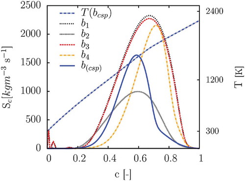
Figure 8. Profiles of temperature, , and intermediate species.

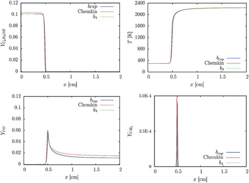
The source term being not equal to zero at is not affecting the behavior of the major species, or the temperature. Despite species such as and being well modeled, the effects on the calculation of intermediate species would have to be further investigated. The CSP, -and -based databases perform well in the 1D premixed flame. The and vectors lead to similar results, but different ignition behavior can be expected.

Premixed laminar Bunsen flame

A second test of the performance of the databases is made by studying a premixed pre-vaporized ethanol-air Bunsen flame. The results are compared with a numerical analysis made by Okuyama et al. (2010), carried out with a -step ethanol reduced kinetic mechanism and a detailed mechanism consisting of species and reactions (San Diego Mechanism, 2015). The inlet of the burner is 0.2 cm wide and the length between the inlet and side-wall is 0.1cm wide. The length of the domain from the horizontal wall to the outlet plane is 0.4 cm; the walls are treated as adiabatic. The mixture of ethanol/air is injected at 1.0 m/s with a laminar plug flow profile, as in the reference simulations (Okuyama et al., 2010). In Figure 9, 10, and 11, the temperature, CO mole fractions, and chemical source term, respectively, are plotted.

Figure 9. Temperature [K] contours.

Figure 10. CO mole fractions [–].

In Figure 9a, the temperature profile predicted by the CSP-based database is shown; the and databases, not reported for sake of brevity, predict a very similar field. The peak of temperature is reached at around 0.3 cm from the ignition plane. A qualitative comparison can be done with the results found in Okuyama et al. (2010), where the tip of the flame is located between 0.18 cm and 0.25 cm from the ignition plane. On the other hand, it can be seen in Figure 9b that the database, as well as the not shown here, lead to different results. The flame does not settle itself at the end of the duct but it stabilizes upstream in the inlet duct. Of course, a similar prediction of the the CO mole fraction and the RPV source term can be observed,respectively, in Figure 10c and 11c. The faster ignition suggests an over-prediction of the laminar flame speed when using the and databases in the calculation. However, the shape of the cone in Figure 9b appears to be less steep when compared to Figure 9a. This is probably due to the fact that where the flame (Figure 9b) attaches, the flow crossing the flame front is blocked by the wall of the duct. In Figure 10 and 11, the flow field predicted using the database is also shown. In Figure 10b it can be seen that CO is gradually increasing across the flame. Instead, Figure 10a, which has the same behavior of the case, shows a higher gradient of CO. This is confirmed also by looking at Figure 11, where the CSP-database (Figure 11a) produces a sharper increase of the source term across the reaction zone than the case. This flow prediction matches the results obtained on the 1D laminar flame, explained in the previous subsection. Referring to Figure 7, it can be seen that the b₂(CO₂, H₂, H₂O) source term spreads over a wider range of the reaction progress variable, and reaches a lower maximum value.

Figure 11. Source term [kg m⁻³s⁻¹] contours.

Conclusions

An optimization of the reaction progress, , under the tabulated chemistry approach has been performed, and its effects on laminar flame calculations investigated. In this work, the reaction progress variable describing the evolution of the reacting system is defined as a combination of the species mass fractions involved in the kinetic mechanism. In such expressions, the weight of each species is calculated with the CSP method; in particular, this algorithm is applied for an ethanol/air mixture. Besides the thermochemical properties characterizing the kinetic mechanism, the main input of the CSP algorithm is a numerical solution of the reacting system. A 1D freely propagating premixed laminar flame is solved with Chemkin Premix and the solution is passed into the CSP algorithm. This methodology has proven to give good results in the case of methane oxidation. However, it leads to unsatisfactory results when applied to a more complex fuel, such as ethanol. As suggested by the work of Lu et al. (2001), an adequate choice for the CSP input data is represented by the time scale analysis performed with the PSR. Within the PSR, the transport processes are not taken into account and the steady-state species can be selected only based on the chemical time scales. A stoichiometric mixture of methane/air is first used to compare the results shown by Lu et al. (2001); subsequently, the efficiency of this approach has been tested with the ethanol/air mixture. A sensitivity analysis of the consumption rate has been performed with the PSR method and the species have been divided in three groups: fast (steady), slow, and dormant. This information has been used to manually correct the set of major species indicated by CSP, in particular by neglecting the species (dormant) whose time scale was out of the range of interest. The so obtained laminar chemical database was then validated against freely propagating premixed laminar flames and premixed Bunsen flame. An additional set of databases built without the usage of the CSP method has been also used for comparison. In total five databases have been assessed and the CSP/PSR-based reaction progress variable leads to satisfactory results, with the main advantage that the chemical database can be created following a clear, systematic, and established procedure.

Acknowledgments

The authors would like to thank C. K. Law for his helpful support and T. Lu for his inspiring technical advice.

Funding

The authors thankfully acknowledge the People Programme (Marie Curie Actions) of the European Union’s Seventh Framework Programme (FP7, ) under grant agreement No. FP7- for the project COPA-GT.

Appendix

In Figure A1, part of the output given by the CSP algorithm is shown; in particular, the species listed in the kinetic mechanism, the steady state species selected by CSP/PSR analysis, and the weight coefficients composing the vector.

Figure A1. Output of CSP/PSR calculation for the definition of the vector.

References

- Albrecht, B.A. 2004. Reactor modeling and process analysis for partial oxidation of natural gas. Disservation. University of Twente, Enschede, the Netherlands.
- Black, G., Curran, H.J., Pichon, S., Simmie, J.M., and Zhukov, V. 2010. Bio-butanol: Combustion properties and detailed chemical kinetic model. Combust. Flame, 157(2), 363–373.
- Dagaut, P., Sarathy, S.M., and Thomson, M.J. 2009. A chemical kinetic study of n-butanol oxidation at elevated pressure in a jet stirred reactor. Proc. Combust. Inst., 32(1), 229–237.
- Dagaut P., and Togbé, C. 2012. Oxidation kinetics of mixtures of iso-octane with ethanol or butanol in a jet-stirred reactor: Experimental and modeling study. Combust. Sci. Technol., 184(7–8), 1025–1038.
- De Jager, B. 2007. Combustion and noise phenomena in turbulent alkane flames. Thesis. University of Twente, Enschede, the Netherlands.
- Dubey, R., Bhadraiah, K., and Raghavan, V. 2010. On the estimation and validation of global single-step kinetics parameters of ethanol-air oxidation using diffusion flame extinction data. Combust. Sci. Technol., 183(1), 43–50.
- Egolfopoulos, F.N., Du, D.X., and Law, C.K. 1992. A study on ethanol oxidation kinetics in laminar premixed flames, flow reactors, and shock tubes. Symp. (Int.) Combust., 24, 833–841.
- Goevert, S., Mira, D., Kok, J.B.W., Vazquez, M., and Houzeaux, G. 2015. Turbulent combustion modelling of a confined premixed methane/air jet flame using tabulated chemistry. Energy Procedia, 66, 313–316.
- Goussis, D.A., Lam, S.H., and Gnoffo, P.A. 1990. Reduced and simplified chemical kinetics for air dissociation using computational singular perturbation. Presented at the 28th Aerospace Sciences Meeting, Reno, NV, January 8–11.
- Guldberg, C.M., and Waage, P. 1879. Concerning chemical affinity. Erdmann’s J. Practische Chemie, 127, 69–114.
- Gülder, Ö. L. 1982. Laminar burning velocities of methanol, ethanol and isooctane-air mixtures. Symp. (Int.) Combust., 19, 275–281.
- Kee, R.J., Rupley, F.M., and Miller, J.A. 1989. Chemkin-II: A Fortran chemical kinetics package for the analysis of gas-phase chemical kinetics. Technical report. Sandia National Laboratory, Livermore, CA.
- Kuo, K.K. 1986. Principles of Combustion, Wiley, New York.
- Lam, S.H., and Goussis, D.A. 1991. Conventional asymptotics and computational singular perturbation for simplified kinetics modelling. In M.D. Smooke (Ed.), Reduced Kinetic Mechanisms and Asymptotic Approximations for Methane-Air Flames, Springer, Berlin Heidelberg, pp. 227–242.
- Lam, S.H., and Goussis, D.A. 1994. The CSP method for simplifying kinetics. Int. J. Chem. Kinet., 26(4), 461–486.
- Lu, T., Ju, Y., and Law, C.K. 2001. Complex CSP for chemistry reduction and analysis. Combust. Flame, 126(1), 1445–1455.
- Ma, L., Naud, B., and Roekaerts, D. 2016. Transported pdf modeling of ethanol spray in hot-diluted coflow flame. Flow Turbul. Combust., 96(2), 469–502.
- Marinov, N.M. 1999. A detailed chemical kinetic model for high temperature ethanol oxidation. Int. J. Chem. Kinet., 31(3), 183–220.
- Massias, A., Diamantis, D., Mastorakos, E., and Goussis, D.A. 1999. An algorithm for the construction of global reduced mechanisms with CSP data. Combust. Flame, 117(4), 685–708.
- Mattos, L.V., and Noronha, F.B. 2005. Hydrogen production for fuel cell applications by ethanol partial oxidation on PT/CEO 2 catalysts: The effect of the reaction conditions and reaction mechanism. J. Catal., 233(2), 453–463.
- Norton, T.S., and Dryer, F.L. 1992. An experimental and modeling study of ethanol oxidation kinetics in an atmospheric pressure flow reactor. Int. J. Chem. Kinet., 24(4), 319–344.
- Okuyama, M., Hirano, S., Ogami, Y., Nakamura, H., Ju, Y., and Kobayashi, H. 2010. Development of an ethanol reduced kinetic mechanism based on the quasi-steady state assumption and feasibility evaluation for multi-dimensional flame analysis. J. Therm. Sci. Technol., 5(2), 189–199.
- Poinsot, T., and Veynante, D. 2005. Theoretical and Numerical Combustion, R.T. Edwards, Inc., Philadelphia, PA.
- Pope, S.B. 2001. Turbulent Flows, Cambridge University Press, Cambridge, UK.
- Röhl, O., and Peters, N. 2009. A reduced mechanism for ethanol oxidation. Presented at the 4th European Combustion Meeting, Vienna, Austria, April 14–17.
- Sallevelt, J.L.H.P., Gudde, J.E.P., Pozarlik, A.K., and Brem, G. 2014. The impact of spray quality on the combustion of a viscous biofuel in a micro gas turbine. Appl. Energy, 132, 575–585.
- San Diego Mechanism. 2015. Chemical kinetic mechanisms for combustion applications. Mechanical and Aerospace Engineering (Combustion Research), University of California at San Diego. Available at: http://combustion.ucsd.edu.
- Saxena, P. 2007. Numerical and experimental studies of ethanol flames and autoignition theory for higher alkanes. Thesis, University of California, San Diego, CA.
- Van Oijen, J.A., Lammers, F.A., and De Goey, L.P.H. 2001. Modeling of complex premixed burner systems by using flamelet-generated manifolds. Combust. Flame, 127(3), 2124–2134.
- Williams, F.A. 1985. Turbulent combustion. Math. Combust., 2, 267–294.
- Yalamanchili, S., Sirignano, W.A., Seiser, R., and Seshadri, K. 2005. Reduced methanol kinetic mechanisms for combustion applications. Combust. Flame, 142(3), 258–265.
Appendix
In , part of the output given by the CSP algorithm is shown; in particular, the species listed in the kinetic mechanism, the steady state species selected by CSP/PSR analysis, and the weight coefficients composing the vector.