Prediction Method for Instability Boundaries of Self-Excited Oscillation Combustion in a Model Combustor

ABSTRACT

This paper presents a method for predicting the stability boundaries of a model combustion chamber using a data-driven approach based on the n-τ model. The n-τ model is derived using a combination of quasi-Monte Carlo sampling and a low-order thermoacoustic network model (LOTANM), and its optimization is established based on experimental data of self-excited oscillating combustion. The objective function is defined as a function of the growth rate, the difference between the corresponding eigenfrequency and the experimental self-excited oscillating combustion frequencies. The critical operating condition boundaries of the model combustion chamber are successfully predicted using the LOTANM, and the results conform with the experimental results. Importantly, while the proposed method reduces the required number of reproducible experiments and eliminates the need for high-power speakers, the linear n-τ model has an inherent limitation in capturing the spectrum of nonlinear behaviors that may arise in the oscillating combustion processes. Overall, the proposed approach represents a practical and effective tool for predicting the stabilities in the testing phases of aeroengine engineering.

KEYWORDS:

• Combustion instabilities
• flame transfer function
• low-order thermoacoustic network model
• n-τ model
• oscillating combustion

Introduction

Owing to the rise in environmental problems, modern aeronautical engines must satisfy strict pollutant emission standards. Combustion is often implemented under lean-fuel operating conditions to reduce pollutant emissions (Lieuwen and Yang 2005). However, lean-fuel combustions can induce oscillating combustions, that can damage the overall structure of the combustor (Ducruix et al. 2003; Prakash, Neumeier, and Zinn 2006). Oscillating combustion is a strong coupling of pressure and heat release rate pulsations in a chamber, manifested as continuous low-frequency, high-amplitude periodic pressure oscillations. To avoid oscillating combustions, it is crucial to analyze the thermoacoustic stability of the combustion system is crucial (Huang and Yang 2009; Natanzon and Culick 2008).

Over the decades, numerous methods have been developed to analyze thermoacoustic stabilities and determine the boundaries of oscillation combustion operating conditions in combustors. These methods include thermoacoustic coupling solution calculations based on computational fluid dynamics (CFD), acoustic finite element methods (FEM), and thermoacoustic coupling analysis based on low-order models (LOM).

CFD methods that utilize compressible large eddy simulations, have the capability to establish digital twins of combustion chambers and collect instability data that are challenging to measure experimentally (Huang and Yang 2009). They provide insights into the impact of various sub-processes, such as evaporation, atomization, and combustion, of stabilities, providing a fundamental understanding at submillimeter scales (Urbano et al. 2017; Wolf et al. 2012). However, both CFD methods involve solving a large number of partial differential equations, which is computationally expensive and time-consuming (Schmitt et al. 2017).

FEM methods directly solve the Helmholtz equations by discretizing them in the frequency domain. Advanced FEM-Helmholtz solvers can calculate thermoacoustic eigenmodes of complex geometries (Ni et al. 2018; Nicoud et al. 2007). It is challenging to obtain the spatial distribution of a flame response using FEM-based methods. Therefore, a combination of CFD and FEM methods is often employed to solve thermoacoustic coupling processes (Andreini et al. 2013). LOM methods have been widely employed in thermoacoustic stability studies and predictions (Förner, Miranda, and Polifke 2015; Mahmoudi et al. 2017; D’alessandro et al. 2018). These models provide simplified representations of the complex interactions between acoustics and combustion, facilitating efficient analysis of stability phenomena. The low order thermo-acoustic network model (LOTANM) based on a one-dimensional plane wave propagation model stands out for analyzing acoustic wave propagation within a combustor. Compared to other LOM methods (Ghirardo, Juniper, and Moeck 2016), LOTANM is based on a one-dimensional propagation model of plane acoustic waves that represents sound pressure and velocity as superpositions of propagation and reflection waves. LOTANM formulates the problem as a set of algebraic equations, simplifying the computational process while preserving essential thermoacoustic coupling dynamics. The LOTANM has been widely used in thermoacoustic stability studies (Chen, Ayton, and Zhao 2019, Han et al. 2021; Wang et al. 2021) and predictions (D’Alessandro et al. 2018; Xia et al. 2019). Stow and Dowling (2004, 2008) proposed it to investigate the limit cycle amplitude of unsteady combustion. Li and Morgans (2015, 2017) comprehensively analyzed linear and nonlinear flame responses and developed the open source combustion instability low-order simulator (OSCILOS). Yang and Morgans (2018) constructed an annular combustion chamber using the LOTANM and developed a theoretical model for longitudinal and circumferential acoustic waves.

Within the framework of LOTANM, the flame transfer function (FTF) is a crucial tool for reducing the order of the flame response model. As the wavelength of the longitudinal acoustic wave in the chamber is typically much larger than the flame thickness (Poinsot and Veynante 2005), the LOTANM ignores the spatial distribution of the flame. The flame front is assumed to be infinitely thin, and the FTF is used to model the responses of flame release rate to disturbances. $FTF(\omega )=({\dot{Q}}^{\prime }/\bar{Q})/\left(u^{\prime }/\bar{u}\right)$, wherein the axial velocity fluctuation $u^{\prime }$is related to global heat release fluctuation${\dot{Q}}^{\prime }$.

Experimental methods are the most direct and widely used methods for measuring dynamic flame responses (Cuquel, Durox, and Schuller 2013; Ducruix, Durox, and Candel 2000). Scholars have used experimental methods to research FTFs (Bellows et al. 2006, 2007; Liu et al. 2021; Palies et al. 2011; Stadlmair and Sattelmayer 2016), resulting in a mature laboratory testing method. Additionally, numerical simulations offer an effective means of obtaining the FTF for conditions or structures that are difficult to test using experimental methods. Similar to the experimental method, numerical simulations apply velocity fluctuations outside the flame and calculate the fluctuation response of the flame heat release rate using an unsteady numerical simulation (Kaiser et al. 2019; Mejia et al. 2018). A new numerical simulation method for obtaining FTF with fewer excitations involves combining the large eddy simulation with system identification (Merk et al. 2018; Scarpato et al. 2016).

Although both the experimental method and numerical simulations facilitate FTF modeling, they involve a considerable amount of repetitive work, which is expensive and time consuming. Moreover, it is difficult for loudspeakers to generate high-velocity pulsations under high-pressure conditions.

Therefore, the aim of this study is to establish a thermoacoustic stability prediction method for aeroengine combustors. Similar to Ghani and Albayrak (2022), an optimization method was employed to establish the linear FTF based on the self-excited oscillation test data of the combustor. We obtained pressure signals through a self-excited oscillation test of a combustor by continuously changing the operating conditions. Finally, the critical instability boundaries of the combustor were predicted using the LOTANM. It is crucial to note that despite the advantages offered by the proposed method, which includes a reduction in the number of necessary reproducible experiments and elimination of the requirement for high-power speakers, there exists an inherent limitation associated with the linear n-τ model. This limitation pertains to its capacity to fully capture the diverse range of nonlinear phenomena such as the triggering of oscillating combustion and mode transitions. Nevertheless, within the context of aeroengine engineering testing phases, the proposed approach continues to demonstrate its practicality and effectiveness in predicting system stabilities.

Testing configuration and optimization methods

Testing configuration

Combustion rig

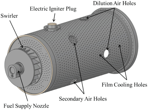
An aeroengine combustion chamber model comprising an annular swirler, fuel injector, and combustion chamber was used, as depicted in Figure 1. We used RP3 kerosene as the fuel, which was injected into the combustor through both the main and pilot atomizers. The pilot stage of the centrifugal atomizer adopted pressure atomization. The main stage adopted direct-spray nozzle. The heights and thicknesses of the swirler vanes were 18 and 2 mm, respectively, with an angle of 70°. The swirl number estimated using the geometry method (Lefebvre and Ballal 2010) was 1.51. Four secondary air holes adjacent to the combustion zone on the wall of the flame tube body, and four dilution air holes near the outlet. A film was used to cool the flame tube wall.

Figure 1. Schematic of the model combustor.

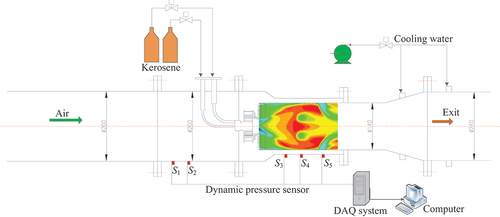
A schematic of the experimental setup is shown in Figure 2. The length of the inlet duct was 2425 mm, and the total length of the test system was 8555 mm. The high-temperature gas generated through combustion was treated and discharged. Air from the compressor was heated using an electric heater and entered the combustion chamber via an intake pipeline.

Figure 2. Schematic of the experimental setup.

Diagnostic techniques

Five dynamic pressure sensors (S1–5) were installed along the airflow direction to capture the self-excited oscillation characteristics of the combustor. XTE-190SM (with semi-infinite tubes) and XCE-062 sensors (with water cooling) (Kulite, New Jersey, USA) were used to measure the pressure pulsations of the inlet and flame tubes, respectively. Q’ was indirectly measured by measuring the CH* chemiluminescence intensity using a photomultiplier tube (HAMAMATSU CH253, Beijing, China) equipped with a 435 ± 10 nm band pass filter (Nori and Seitzman 2009). In prior studies, the CH* emission from the flame was employed as an indicator to offer a qualitative estimation of the heat release rate in both premixed (Khalil and Gupta 2017) and non-premixed (Ahn et al. 2019; Han et al., 2021) scenarios. However, it is worth noting that the utilization of the measurement methods in non-premixed flames remains a subject of controversy. Since elucidating the generation mechanism of CH* during non-premixed combustion of hydrocarbon fuels falls outside the scope of this paper, our approach in this study primarily utilizes the CH* signal as an indicator to visualize trends in heat release rate fluctuations. It is important to emphasize that the CH* signal, while considered in our analysis, is not the primary focus of our investigation. All signals were collected using the Sirius R8 (Dewesoft, Trbovlje, Trbovlje Commune, Slovenia) multichannel data acquisition system. The sampling frequency was set to 10 kHz.

Operating conditions

The system was tested under continuously changing operating conditions to investigate the characteristics of the self-excited oscillations during combustion and the instability boundaries of the combustor under different operating conditions. The operating conditions adopted in this study are listed in Table 1. A constant airflow rate (W_a) was maintained throughout the experiments to maintain a constant flow in the chamber. The inlet total pressure (P₃*) was 850 kPa. The inlet air temperature was adjusted using the electrical heater, and the total air temperature (T₃*) was varied from 390–550 K. During the experimental process, the RP3 mass flow rate of the pilot atomizer (W_f,p) was maintained at 5.92 g/s, while the RP3 mass flow rate of the main atomizer (W_f,m) was adjusted from 12.24 g/s to 20.91 g/s by regulating the upstream fuel pressure. The total fuel-air ratio (far) of test conditions for thermoacoustic instabilities varies from 0.0144 to 0.0213. The total temperature of the gas (T₄*) was measured from 1350 to 1550K.In each instability condition, sufficient time was ensured to stabilize the combustor before data collection. The hot test duration was approximately 120 min.

Table 1. Operating conditions summary.

Wa (kg/s)	P3* (kPa)	T3* (K)	Wf,p (g/s)	Wf,m (g/s)	far(-)	T4* (K)
1.26	850	390–550	5.92	12.24–20.91	0.0144–0.0213	1350–1550

Theoretical modeling and optimization method

The LOTANM was used as the prediction method to assess the stability of the model chamber. The classical n-τ model was used to describe the response of ${\dot{Q}}^{\prime }$from the flame to acoustic disturbance. Based on the test data presented under the Experimental Results section, a relationship between n, τ, and operating conditions was established.

Combustor LOTANM

The LOTANM simplifies the combustion system structure into several adjacent acoustic modules, wherein sound waves are transmitted across modules. The flame is simplified as an infinitely thin plane at the chamber inlet. The response of the unsteady heat release rate pulsation to acoustic disturbances can be described using the FTF. Based on the geometric dimensions of the test bench (listed in Table 2), a one-dimensional thermoacoustic network model, depicted in Figure 3, was established.

Figure 3. Schematic of the LOTAN.

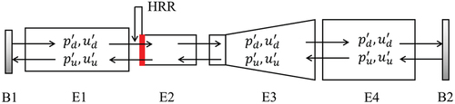
Table 2. Dimensions of acoustic modules.

Name	Acoustic module	Length (m)	Diameter (m)
B1	Inlet boundary	-	-
E1	Inlet tank	2.425	0.2
E2	Chamber	0.25	0.14
E3	Transition segment	0.1、0.61	0.14、0.24
E4	Exhaust	5.17	0.240
B2	Exhaust boundary	-	-

The wave equation of the one-dimensional mean flow was solved to obtain the Riemann invariant, which can be considered the characteristic wave amplitude propagating upstream (f) and downstream (g).$f=\frac{1}{2}\left(p^{\prime }/\bar{\rho }\bar{c}+u^{\prime }\right)$ and $g=\frac{1}{2}\left(p^{\prime }/\bar{\rho }\bar{c}-u^{\prime }\right)$, where p, u, ρ, and c denote pressure, velocity, density, and sound speed respectively; the superscript ’ denotes the pulsation value of variables, and superscript – denotes their mean value. The relationship between the input and output of each downstream module perturbation in a linear time-invariant system is represented by transfer matrix T as follows:

(1) $\left(\begin{array}{c}{p_d}^{\prime }\\ {u_d}^{\prime }\end{array}\right)=\left(\begin{array}{cc}{T}_{11}& T_{12}\\ T_{21}& T_{22}\end{array}\right)\left(\begin{array}{c}{p_u}^{\prime }\\ {u_u}^{\prime }\end{array}\right)+\left(\begin{array}{c}{p_s}^{\prime }\\ {u_s}^{\prime }\end{array}\right)$(1)

where subscripts d and u denote downstream and upstream directions, respectively. The source term s is added to Equation (1)(1) $\left(\begin{array}{c}{p_d}^{\prime }\\ {u_d}^{\prime }\end{array}\right)=\left(\begin{array}{cc}{T}_{11}& T_{12}\\ T_{21}& T_{22}\end{array}\right)\left(\begin{array}{c}{p_u}^{\prime }\\ {u_u}^{\prime }\end{array}\right)+\left(\begin{array}{c}{p_s}^{\prime }\\ {u_s}^{\prime }\end{array}\right)$(1) only for the flame positions. The Riemann invariants of the module input and output can be described as a scattering matrix S. For simple geometries, the scattering matrix of the modules can be derived using the linearized mass and momentum conservation equations, and the scattering matrix of the system can be obtained by connecting the acoustic modules from the inlet to the outlet boundary.

(2) $\left(\begin{array}{c}{f}_d\\ g_u\end{array}\right)=\left(\begin{array}{cc}{S}_{11}& S_{12}\\ S_{21}& S_{22}\end{array}\right)\left(\begin{array}{c}{f}_u\\ g_d\end{array}\right)+\left(\begin{array}{c}{f}_s\\ g_s\end{array}\right)$(2)

In this system, the effect of the compressor at the inlet can be described using the reflection coefficient. Based on the theoretical derivation results of Silva et al. (2014), the reflection coefficient of a compact compressor whose longitudinal length is significantly smaller than the wavelength of the sound wave can be calculated as

(3) $R_1=\frac{\left(1-\overline{Ma}\right)\left(k\zeta +\gamma \overline{Ma}\right)}{\left(1+\overline{Ma}\right)\left(k\zeta -\gamma \overline{Ma}\right)}$(3)

where Ma denotes the Mach number of the air at the outlet, k is a constant related to the compressor characteristics, and $\zeta =1+\overline{Ma}\left(\gamma -1\right)/2$, where $\gamma$ symbolizes the gas-specific heat capacity ratio. When the amplitude of the pressure fluctuation in the compressor is small, k ≈0. The value of R₁ is approximately −0.96. The high-temperature gas was discharged at the outlet boundary by passing it through an exhaust gas treatment device with a long longitudinal length and a large cross-sectional area; therefore, the reflected wave barely affected the system. The outlet was regarded as an opening boundary. The fuel is injected into the combustor through small orifices in the injector, with dimensions much smaller than the characteristic size of the combustion chamber. Owing to the high pressure difference, the injector is typically choked, primarily affecting the air line rather than the fuel line (Han et al., 2021). Consequently, the influence of the injector on the acoustics has been disregarded in the LOTANM model.

The LOTANM of the system was solved using the OSCILOS (Li and Morgans 2015; Li et al. 2017). The eigenvalues were located at the minimum error E, at the outlet boundary. The results of the eigenvalues show that when the growth rate (GR) > 0, disturbances are amplified, resulting in an increase in the pressure pulsation amplitude until it reaches a saturation limit cycle state.; when GR < 0, the damping effect gradually reduces the disturbance and the pressure pulsation amplitude decays over time; and when GR ≈0, the system behaves as if it is in a limit cycle state.

FTF and optimization method

The flame model describes the heat release rate fluctuations, which depend on the flow fluctuations induced by the acoustics immediately ahead of the flame. For decades, the linear FTF has been used to describe the linear response of heat release rate fluctuations to disturbances during weak perturbations (Dowling 1997; Peracchio and Proscia 1999; Goh and Morgans 2013). The n-τ model, proposed by Crocco (1951), is expressed as

(4) $\frac{{\dot{Q}}^{\prime }\left(t\right)}{\overline{Q^{\prime }}}=n\frac{u^{\prime }\left(t-\tau \right)}{\bar{u}}$(4)

where n denotes interaction index and τ indicates time delay. Thermoacoustic instability in a combustion chamber involves a complex interplay of various subprocesses, such as sound wave propagation, fuel injection, atomization, evaporation, flow, mixing, heat transfer, and chemical reactions between multicomponent gases. The n-τ model represents the interaction gain between these subprocesses through n and the fuel combustion time through τ. The values of n and τ are complex functions of the chamber geometry and operating parameters, making it challenging to derive their mathematical expressions and predict the stability of the combustion chamber during the design stage.

In this study, a method is proposed to establish the relationship between (n, τ) and the operating condition parameters to evaluate the chamber stability. According to the linear propagation theory of perturbations, a fully developed self-excited oscillation combustion exhibits a stable pulsation state with a constant pressure pulsation amplitude and GR ≈0. Therefore, the difference between the frequency in the calculated results and that observed experimentally and the GR of the LOTANM calculation can be used as the objective function to optimize the values of n and τ.

(5) $D=\sqrt{{\left(F_0-F_1\right)}^2+{\left(G_1\right)}^2}$(5)

where F₀ denotes oscillation frequency obtained experimentally, and F₁ and G₁ is the frequency and GR calculated using LOTANM, respectively. Additionally, $D$ represents the complex plane distance between the experimental frequency, located on the real axis, and the eigenvalue predicted by the thermoacoustic network model. Additionally, it considers the difference between G₁ and zero. The method can be briefly described as follows:

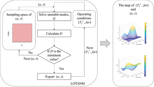
1. A LOTANM is established based on the geometric dimensions of the experimental system.

2. A sampling space for n and τ is generated using the quasi-Monte Carlo sampling method, which produces 2D Sobol sequences within a predetermined range of (n, τ). Sobol sequences (Sobol′ 2001) are low-variance pseudo-random sequences that ensure the sample points have good spatial distributions. Based on experimental research experience (Hield, Brear, and Jin 2009; Bernier, Lacas, and Candel 2004; Fu, Yang and Guo 2009), the value of n in this study ranges from 0–4, whereas that of τ ranges from 0–20 (ms).

3. The LOTANM was employed to calculate the minimum D under different operating conditions (n, τ). The corresponding values of n and τ were obtained from the calculated results.

4. The Kriging surrogate model (Jones 2001) was used to characterize the relationship between the operating condition parameters T₃* and far, and (n, τ). The Kriging model is an estimation model that predicts the responses at unknown data points using observed data.

Figure 4 presents a flowchart of the aforementioned method.

Figure 4. Flowchart of the n-τ model calculation method.

Results and discussion

The proposed method was used to establish the relationship between the n-τ model and operating condition parameters. The model was used to predict the stability of the model chamber.

Experimental results

Experimental data on oscillating combustion were recorded after stabilizing the operating conditions, and both stable and self-excited oscillating states were observed during the tests. Table 3 lists the representative stable and unstable operating conditions. The main frequency was calculated from the dynamic pressure time series measured using the S3 sensor, which was near the combustion zones, using the fast Fourier transform method. The characteristics of the stable test (Test 14) and oscillating state (Test 15) are shown in Figures 5 and 6, respectively. The oscillation intensity of combustion is expressed as the ratio of the peak – peak value of $p{ }^{\mathrm{\prime }}$ to the average value, $p{ }_{\mathrm{p}\mathrm{p}\mathrm{v}}^{\prime }/p{ }_{\mathrm{a}\mathrm{v}\mathrm{g}}^{\prime }$, $p{ }_{\mathrm{p}\mathrm{p}\mathrm{v}}^{\prime }=p{ }_{\mathrm{m}\mathrm{a}\mathrm{x}}^{\prime }-p{ }_{\mathrm{m}\mathrm{i}\mathrm{n}}^{\prime }$, where the subscripts ppv, avg, max, and min represent the peak-to-peak value, average value, maximum value, and minimum value of $p{ }^{\mathrm{\prime }}$, respectively.

Figure 5. Dynamic pressure and heat release rate in test 14: $p{ }_{\mathrm{p}\mathrm{p}\mathrm{v}}^{\prime }/p{ }_{\mathrm{a}\mathrm{v}\mathrm{g}}^{\prime }$ is calculated using sliding windows with a window length of 4096 samples and an overlap of 2048 samples.

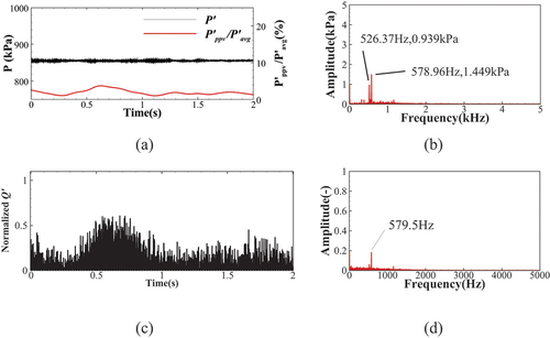
Figure 6. Dynamic pressure and normalized heat release rate in test 15: $p{ }_{\mathrm{p}\mathrm{p}\mathrm{v}}^{\prime }/p{ }_{\mathrm{a}\mathrm{v}\mathrm{g}}^{\prime }$ is calculated using sliding windows with a window length of 4096 samples and overlap of 2048 samples.

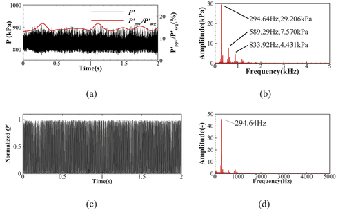
Table 3. Representative operating conditions of experiment.

Test No.	T3*(K)	far(-)	Main Frequency(Hz)	State	Usage
1	418	0.0158	280.1	Oscillating	Training
2	437	0.0162	288.47	Oscillating	Training
3	467	0.0163	296.63	Oscillating	Training
4	472	0.0163	296.3	Oscillating	Training
5	489	0.0156	301.56	Oscillating	Training
6	489	0.0163	305.34	Oscillating	Training
7	522	0.0165	310.63	Oscillating	Training
8	536	0.016	313.15	Oscillating	Training
9	541	0.016	317.27	Oscillating	Training
10	544	0.0158	316.82	Oscillating	Training
11	544	0.0162	-	Stable	-
12	545	0.0156	312.35	Oscillating	Training
13	549	0.0156	317.97	Oscillating	Training
14	400	0.0171	-	Stable	Verifying
15	400	0.0168	276.57	Oscillating	Verifying
16	453	0.0171	-	Stable	Verifying
17	453	0.0168	-	Stable	Verifying
18	453	0.0164	294.64	Oscillating	Verifying

Under the conditions of T₃* = 453 K and far = 0.0171 (Figure 5), the $p{ }_{\mathrm{p}\mathrm{p}\mathrm{v}}^{\prime }/p{ }_{\mathrm{a}\mathrm{v}\mathrm{g}}^{\prime }$ values were less than 5%, and the main frequency was 578.96 Hz with an amplitude of approximately 1.45 kPa. In contrast, under the conditions of T₃* = 453 K and far = 0.0168 (Figure 6), the $p{ }_{\mathrm{p}\mathrm{p}\mathrm{v}}^{\prime }/p{ }_{\mathrm{a}\mathrm{v}\mathrm{g}}^{\prime }$ values were approximately 15%, and the pulsation amplitude at 294.64 Hz was approximately 29 kPa. Additionally, the CH*chemiluminescence intensity signal during Test 15 indicated that ${\dot{Q}}^{\prime }$ had a higher pulsation amplitude.

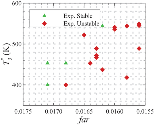
Figure 7 presents a stability map of the combustor. It is evident that as the inlet temperature increases, the instability boundary of the model combustor gradually shifted toward lower far values. In this study, the improved distribution of droplets and flames with higher T₃* values contributed to a broader stable operating range of the chamber. Conversely, an increase in the inlet temperature led to a corresponding increase in the average sound velocity of the airflow, resulting in an increase in the main frequency of the oscillating combustion in the chamber.

Figure 7. Experimental results for the stability map: the green ▲ symbols denote the stable state; the red ♦ symbols denote the oscillating state.

FTF optimization results

Tests 1–10, 12, and 13, whose operating conditions are listed in Table 3, were used to compute the n-τ model. The results are presented in Table 4. The Kriging model was employed as the mapping tool to depict the correlation between (n, τ) and (T₃*, far), as illustrated in Figure 8. n exhibited a direct relationship with T₃* and far. When other operating conditions are the same, an increase in the inlet temperature can facilitate the atomization of liquid droplets, thereby contributing to enhanced combustion power and chamber efficiency. Conversely, an increase in the fuel flow rate resulted in an increase in the combustion power. n characterizes the magnification effect of the heat release rate fluctuations on the acoustic disturbance. The spatial energy density of the chamber increases when the power is increased, enabling the sound field to derive more energy from the combustion field. Consequently, the value of n increases, as shown in Figure 8(a). Additionally, an increase in both T₃* and far promotes fuel atomization and evaporation. An increase in T₃* results in an increase in the fuel temperature before injection, while an increase in the far value enhances the average temperature of the chamber. Moreover, reducing the time of fuel injection from the nozzle to the completion of combustion shortened the delay time τ, as shown in Figure 8(b).

Figure 8. Calculation results of n-τ model parameters: mapped by the kriging model. Maps of (a) n and (b) τ varying with different T₃* and far values.

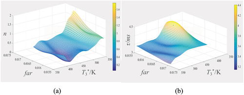
Table 4. Optimization result of (n, τ.).

Test No.	T3* (K)	far(-)	n(-)	τ(ms)
1	418	0.0158	0.268	3.599
2	437	0.0162	0.111	4.097
3	467	0.0163	0.205	3.7
4	472	0.0163	0.354	3.501
5	489	0.0156	0.415	3.563
6	489	0.0163	0.496	3.492
7	522	0.0165	0.984	3.336
8	536	0.016	1.252	3.368
9	541	0.016	1.001	3.328
10	544	0.0158	1.604	3.227
12	545	0.0156	1.372	3.241
13	549	0.0156	1.552	3.165

The Kriging model can be used to compute the values of (n, τ) under different operating conditions, and the LOTANM can be used to predict the thermoacoustic stability of the chamber. In this study, the accuracy of the proposed method was validated by calculating the unstable modes for Tests 14 and 15. The prediction results indicated that the values of (n, τ) were (0.332, 3.682) and (0.1096, 3.734) for Tests 14 and 15, respectively. The eigenmodes of the system were calculated using the LOTANM, and the corresponding outcomes are shown in Figure 9.

Figure 9. Eigenmode distributions in tests 14 and 15: the main modes of the system are indicated by red circles. (a) test 14: T₃* = 400 K, far = 0.0171 and (b) test 15: T₃* = 400 K, far = 0.0168.

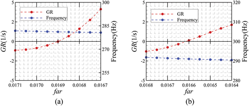
The minimum point of 20log€ on the contour map represents the eigenmode of the system. In Figure 9(a), far has a higher value, and the corresponding GR values are − 3.76, −2.33, and −5.06 rad/s with eigenfrequencies of 269.19, 289.48, and 327.46 Hz, respectively. This indicates that the system was stable under the conditions used in Test 14. However, when far decreased to 0.0168 in Test 15, as depicted in Figure 9(b), the GR values changed to − 4.05, 2.12, and −8.21 rad/s at 269.89, 291.16, and 328.64 Hz, respectively. At an eigenfrequency of approximately 290 Hz, GR > 0 and the disturbance in the system was amplified, thereby establishing a limit cycle. These observations imply that a critical value of far exists between 0.0164 and 0.0168, which ensures that GR = 0 at an eigenfrequency of approximately 290 Hz. This aligns with the test results depicted in Figure 6, indicating that the chamber is stable at (453 K, 0.0168) and oscillates at (453 K, 0.0164). Therefore, the critical operating condition boundaries of the combustion instabilities can be identified based on the point where the GR transitions to zero.

Stability map prediction

The GRs for different T₃* values are shown in Figure 10. It is evident that as the far value decreases, the eigenfrequency decreases and GR increases, which is evident for both T₃* = 400 K (Figure 10(a)) and T₃* = 453 K (Figure 10(b)). The decrease in far resulted in a decrease in the flame temperature, leading to a corresponding decrease in the characteristic frequency of the mode. The critical far boundaries of combustion instabilities can be predicted through linear interpolation. At the critical far value, the GR is zero. For T₃* = 400 K, the critical far value was 0.01690, and the corresponding eigenfrequency was 281.14 Hz. Similarly, for T₃* = 453 K, the critical far value was 0.01661 and the corresponding eigenfrequency was 291.08 Hz. These results agree with the experimental values of 276.57 Hz obtained in Tests 14 and 15 and 294.64 Hz in Tests 16–18, with relative errors of 1.67% and − 4.58%, respectively.

Figure 10. Evolution of the growth rate (marked with red ●) and the corresponding eigenfrequencies (marked width blue ●) for changes in the far value. (a) T₃* = 400 K and (b) T₃* = 453 K.

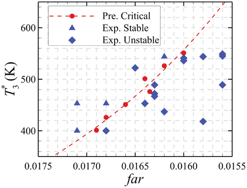
The calculation results demonstrate that the proposed method can predict the instability boundaries of a combustion chamber under various operating conditions. The critical far values were calculated for different T₃* values, and the results are presented in Figure 11. The stable and unstable operating points in the experiments are denoted by ■ and ▲, respectively, and the critical operating points predicted by the LOTANM are denoted by ●. As T₃* increased, the critical far values for the oscillating combustion in the model chamber decreased, indicating a wider stable operating range of the chamber. The critical operating condition boundaries predicted by LOTANM agreed well with the experimental results.

Figure 11. Operating condition instability boundaries of the combustor under self-excited oscillation combustion: the dashed line denotes the power fitted curve of ●.

Conclusion

This paper presented a method for predicting the operating condition boundaries of a combustion chamber by utilizing experimental data from self-excited oscillations in a model chamber. The proposed approach involves optimizing the relationship between the n-τ model and operating condition parameters by combining experimental data and theoretical modeling and subsequently using the LOTANM with the n-τ model to predict the critical operating condition boundaries. The proposed approach is a promising and effective method for enhancing the design and safety of combustion systems.

Overall, the LOTANM is a comprehensive and efficient approach for predicting the critical operating condition boundaries of combustion chambers, which is crucial for ensuring their stability and safety. The method has the potential to considerably reduce the time and cost required for experimentation, and can provide valuable insights into the underlying physics of combustion instabilities. However, it is worth mentioning that the accuracy and reliability of the predictions depend heavily on the quality and quantity of experimental data used in the modeling process. Therefore, further research and validations are required to fully establish the applicability and robustness of the LOTANM.

It is essential to note that this paper primarily focuses on analyzing and predicting the stability boundaries of the combustor based on the linear n-τ model. However, the capability of predicting nonlinear phenomena in the self-excited oscillating combustion process, such as modal transition, is limited. Additional investigations are required to explore and incorporate the effects of nonlinearity into the model to obtain a more comprehensive understanding of the behavior of the system.

Disclosure statement

No potential conflict of interest was reported by the author(s).

Additional information

Funding

This work was supported by the Sichuan Gas Turbine Establishment of AECC Stable Support Project under Grant Number GJCZ-2019-0029.

References

- Ahn, B., J. Lee, S. Jung, and K. T. Kim. 2019. Nonlinear mode transition mechanisms of a self-excited jet A-1 spray flame. Combust. Flame 203:170–79. doi:10.1016/j.combustflame.2019.02.008.
- Andreini, A., B. Facchini, A. Giusti, I. Vitale, and F. Turrini. 2013. Thermoacoustic analysis of a full annular lean burn aero-engine combustor. In ASME Turbo Expo 2013: Turbine Technical Conference and Exposition Volume 1A: Combustion, Fuels and Emissions. San Antonio: The American Society of Mechanical Engineers Digital Collection. doi:10.1115/gt2013-94877.
- Bellows, B. D., M. K. Bobba, A. Forte, J. M. Seitzman, and T. Lieuwen. 2007. Flame transfer function saturation mechanisms in a swirl-stabilized combustor. Proc. Combust. Inst. 31 (2):3181–88. doi:10.1016/j.proci.2006.07.138.
- Bellows, B. D., M. K. Bobba, J. M. Seitzman, and T. Lieuwen. 2006. Nonlinear flame transfer function characteristics in a Swirl-stabilized combustor. J. Eng. Gas Turbines Power 129 (4):954–61. doi:10.1115/1.2720545.
- Bernier, D., F. Lacas, and S. Candel. 2004. Instability mechanisms in a premixed prevaporized combustor. J. Propuls. Power 20 (4):648–56. doi:10.2514/1.11461.
- Chen, Y., L. J. Ayton, and D. Zhao. 2019. Modelling of intrinsic thermoacoustic instability of premixed flame in combustors with changes in cross section. Combust. Sci. Technol 192 (5):832–51. doi:10.1080/00102202.2019.1594799.
- Crocco, L. 1951. Aspects of combustion stability in liquid propellant rocket motors part I: Fundamentals. Low frequency instability with monopropellants. J. Am. Rocket Soc 21 (6):163–78. doi:10.2514/8.4393.
- Cuquel, A., D. Durox, and T. Schuller. 2013. Scaling the flame transfer function of confined premixed conical flames. Proc. Combust. Inst. 34 (1):1007–14. doi:10.1016/j.proci.2012.06.056.
- D’Alessandro, S., M. L. Frezzotti, B. Favini, and F. Nasuti. 2018. A multi-dimensional approach for low order modeling of combustion instability in a rocket combustor. 2018 Joint Propulsion Conference, p. 4677. Cincinnati, Ohio: American Institute of Aeronautics and Astronautics. doi: 10.2514/6.2018-4677.
- Dowling, A. P. 1997. Nonlinear self-excited oscillations of a ducted flame. J. Fluid. Mech. 346:271–90. doi:10.1017/S0022112097006484.
- Ducruix, S., D. Durox, and S. Candel. 2000. Theoretical and experimental determinations of the transfer function of a laminar premixed flame. Proc. Combust. Inst. 28 (1):765–73. doi:10.1016/S0082-0784(00)80279-9.
- Ducruix, S., T. Schuller, D. Durox, and S. Candel. 2003. Combustion dynamics and instabilities: Elementary coupling and driving mechanisms. J. Propuls. Power 19 (5):722–34. doi:10.2514/2.6182.
- Förner, K., A. C. Miranda, and W. Polifke. 2015. Mapping the influence of acoustic resonators on rocket engine combustion stability. J. Propuls. Power 31 (4):1159–66. doi:10.2514/1.B35660.
- Ghani, A., and A. Albayrak. 2022. From pressure time series data to flame transfer functions: A framework for perfectly premixed swirling flames. J. Eng. Gas Turbines Power 145 (1):011005. doi:10.1115/1.4055724.
- Ghirardo, G., M. P. Juniper, and J. P. Moeck. 2016. Weakly nonlinear analysis of thermoacoustic instabilities in annular combustors. J. Fluid. Mech. 805:52–87. doi:10.1017/jfm.2016.494.
- Goh, C. S., and A. S. Morgans. 2013. The influence of entropy waves on the thermoacoustic stability of a model combustor. Combust. Sci. Technol 185 (2):249–68. doi:10.1080/00102202.2012.715828.
- Han, X., D. Yang, J. Wang, and C. Zhang. 2021. The effect of inlet boundaries on combustion instability in a pressure-elevated combustor. Aerosp. Sci. Technol. 111:106517. doi:10.1016/j.ast.2021.106517.
- Hield, P. A., M. J. Brear, and S. H. Jin. 2009. Thermoacoustic limit cycles in a premixed laboratory combustor with open and choked exits. Combust. Flame 156 (9):1683–97. doi:10.1016/j.combustflame.2009.05.011.
- Huang, Y., and V. Yang. 2009. Dynamics and stability of lean-premixed swirl-stabilized combustion. Prog. Energy Combust. Sci. 35 (4):293–364. doi:10.1016/j.pecs.2009.01.002.
- Jones, D. R. 2001. A taxonomy of global optimization methods based on response surfaces. J. Glob. Optim. 21 (4):345–83. doi:10.1023/A:1012771025575.
- Kaiser, T. L., G. Öztarlik, L. Selle, and T. Poinsot. 2019. Impact of symmetry breaking on the flame transfer function of a laminar premixed flame. Proc. Combust. Inst. 37 (2):1953–60. doi:10.1016/j.proci.2018.06.047.
- Khalil, A. E. E., and A. K. Gupta. 2017. Acoustic and heat release signatures for swirl assisted distributed combustion. Appl. Energy 193:125–38. doi:10.1016/j.apenergy.2017.02.030.
- Lefebvre, A. H., and D. R. Ballal. 2010. Gas turbine combustion: Alternative fuels and emissions. 3rd ed. Boca Raton: Taylor & Francis. doi:10.1201/9781420086058.
- Lieuwen, T. C., and V. Yang, eds. 2005. Combustion instabilities in gas turbine engines: Operational experience, fundamental mechanisms, and modeling. Reston: American Institute of Aeronautics and Astronautics.
- Li, J., and A. S. Morgans. 2015. Time domain simulations of nonlinear thermoacoustic behaviour in a simple combustor using a wave-based approach. J. Sound Vib. 346:345–60. doi:10.1016/j.jsv.2015.01.032.
- Liu, W., L. Zhang, R. Xue, Q. Yang, and H. Wang. 2021. Experimental investigation on nonlinear response of a low-swirl flame to acoustic excitation with large amplitude. J. Eng. Gas Turbines Power 143 (12):121021. doi:10.1115/1.4052024.
- Li, J., Y. Xia, A. S. Morgans, and X. Han. 2017. Numerical prediction of combustion instability limit cycle oscillations for a combustor with a long flame. Combust. Flame 185:28–43. doi:10.1016/j.combustflame.2017.06.018.
- Li, J., D. Yang, C. Luzzato, and A. S. Morgans. 2017. Open source combustion instability low order simulator (OSCILOS-Long) technical report. Imperial College London, UK: Department of Aeronautics. Accessed November 22, 2022. 9https://www.oscilos.com/download/OSCILOS_Long_Tech_report.pdf or https://github.com/MorgansLab/OSCILOS_long/blob/main/docs/OSCILOS_Long_Tech_report.pdf.
- Mahmoudi, Y., A. Giusti, E. Mastorakos, and A. P. Dowling. 2017. Low-order modeling of combustion noise in an aero-engine: The effect of entropy dispersion. J. Eng. Gas Turbines Power 140 (1). doi:10.1115/1.4037321.
- Mejia, D., M. Miguel-Brebion, A. Ghani, T. Kaiser, F. Duchaine, L. Selle, and T. Poinsot. 2018. Influence of flame-holder temperature on the acoustic flame transfer functions of a laminar flame. Combust. Flame 188:5–12. doi:10.1016/j.combustflame.2017.09.016.
- Merk, M., S. Jaensch, C. Silva, and W. Polifke. 2018. Simultaneous identification of transfer functions and combustion noise of a turbulent flame. J. Sound Vib. 422:432–52. doi:10.1016/j.jsv.2018.02.040.
- Natanzon, M. S., and F. E. C. Culick. 2008. Combustion instability. Reston: American Institute of Aeronautics and Astronautics.
- Nicoud, F., L. Benoit, C. Sensiau, and T. Poinsot. 2007. Acoustic modes in combustors with complex impedances and multidimensional active flames. Aiaa J. 45 (2):426–41. doi:10.2514/1.24933.
- Ni, F., F. Nicoud, Y. Méry, and G. Staffelbach. 2018. Including flow–acoustic interactions in the Helmholtz computations of industrial combustors. AIAA J. 56 (12):4815–29. doi:10.2514/1.J057093.
- Nori, V. N., and J. M. Seitzman. 2009. CH* chemiluminescence modeling for combustion diagnostics. Proc. Combust. Inst. 32 (1):895–903. doi:10.1016/j.proci.2008.05.050.
- Palies, P., D. Durox, T. Schuller, and S. Candel. 2011. Experimental study on the effect of swirler geometry and swirl number on flame describing functions. Combust. Sci. Technol 183 (7):704–17. doi:10.1080/00102202.2010.538103.
- Peracchio, A. A., and W. M. Proscia. 1999. Nonlinear heat-release/acoustic model for thermoacoustic instability in lean premixed combustors. J. Eng. Gas Turbines Power 121 (3):415–21. doi:10.1115/1.2818489.
- Poinsot, T., and D. Veynante. 2005. Theoretical and numerical combustion. 2nd ed. Philadelphia: Edwards.
- Prakash, S., Y. Neumeier, and B. Zinn. 2006. Investigation of mode shift dynamics of lean, premixed flames. In 44th AIAA aerospace sciences meeting and exhibit, 961. Reno, Nevada: Aerospace Research Central. doi:10.2514/6.2006-961.
- Scarpato, A., L. Zander, R. Kulkarni, and B. Schuermans. 2016. Identification of multi-parameter flame transfer function for a reheat combustor. In ASME Turbo Expo 2016: Turbomachinery Technical Conference and Exposition, Combustion, Fuels and Emissions 4B: p. V04BT04A038. Seoul: The American Society of Mechanical Engineers Digital Collection doi: 10.1115/gt2016-57699.
- Schmitt, T., G. Staffelbach, S. Ducruix, S. Gröning, J. S. Hardi, and M. Oschwald. 2017. Large-eddy simulations of a sub-scale liquid rocket combustor: Influence of fuel injection temperature on thermo-acoustic stability. In 7th European Conference for Aeronautics and Aerospace Sciences. Milan, Italy. doi: 10.13009/EUCASS2017-352.
- Silva, C., I. Duran, N. Franck, and S. Moreau. 2014. Boundary conditions for the computation of thermo-acoustic modes in combustion chambers. Aiaa J. 52 (6):1180–93. doi:10.2514/1.J052114.
- Sobol′, I. M. 2001. Global sensitivity indices for nonlinear mathematical models and their monte carlo estimates. Math. Comput. Simul. 55 (1–3):271–80. doi:10.1016/S0378-4754(00)00270-6.
- Stadlmair, N., and T. Sattelmayer. 2016. Measurement and analysis of flame transfer functions in a lean-premixed, swirl-stabilized combustor with water injection. In 54th AIAA Aerospace Sciences Meeting. San Diego: American Institute of Aeronautics and Astronautics. doi:10.2514/6.2016-1157.
- Stow, S. R., and A. P. Dowling. 2004. Low-order modelling of thermoacoustic limit cycles. In ASME turbo expo 2004: Power for land, sea, and Air, turbo expo 2004, Vol. 1, 775–86. Vienna: The American Society of Mechanical Engineers Digital Collection. doi:10.1115/gt2004-54245.
- Stow, S. R., and A. P. Dowling. 2008. A time-domain network model for nonlinear thermoacoustic oscillations. In ASME turbo expo 2008: Power for land, sea, and air. In Combustion, fuels and emissions, parts a and B, Vol. 3, 539–51. Berlin: The American Society of Mechanical Engineers Digital Collection. doi:10.1115/gt2008-50770.
- Urbano, A., Q. Douasbin, L. Selle, G. Staffelbach, B. Cuenot, T. Schmitt, S. Ducruix, and S. Candel. 2017. Study of flame response to transverse acoustic modes from the LES of a 42-injector rocket engine. Proc. Combust. Inst. 36 (2):2633–39. doi:10.1016/j.proci.2016.06.042.
- Wang, Y., C. H. Sohn, J. Bae, and Y. Yoon. 2021. Prediction of combustion instability by combining transfer functions in a model rocket combustor. Aerosp. Sci. Technol. 119:107202. doi:10.1016/j.ast.2021.107202.
- Wolf, P., G. Staffelbach, L. Y. M. Gicquel, J.-D. Müller, and T. Poinsot. 2012. Acoustic and large eddy simulation studies of azimuthal modes in annular combustion chambers. Combust. Flame 159 (11):3398–413. doi:10.1016/j.combustflame.2012.06.016.
- Xia, Y., D. Laera, W. P. Jones, and A. S. Morgans. 2019. Numerical prediction of the flame describing function and thermoacoustic limit cycle for a pressurised gas turbine combustor. Combust. Sci. Technol 191 (5–6):979–1002. doi:10.1080/00102202.2019.1583221.
- Yang, D., and A. S. Morgans. 2018. Low-order network modeling for annular combustors exhibiting longitudinal and circumferential modes. In ASME Turbo Expo 2018: Turbomachinery Technical Conference and Exposition, Combustion, Fuels, and Emissions 4B: p. V04BT04A026. Oslo: The American Society of Mechanical Engineers Digital Collection. doi: 10.1115/gt2018-76506.