Multi-agent motion planning for nonlinear Gaussian systems

Abstract

In this paper, a multi-agent motion planner is developed for nonlinear Gaussian systems using a combination of probabilistic approaches and a rapidly exploring random tree (RRT) algorithm. A closed-loop model consisting of a controller and estimation loops is used to predict future distributions to manage the level of uncertainty in the path planner. The closed-loop model assumes the existence of a feedback control law that drives the actual system towards a nominal system. This ensures the uncertainty in the evolution does not grow significantly and the tracking errors are bounded. To trade conservatism with the risk of infeasibility and failure, we use probabilistic constraints to limit the probability of constraint violation. The probability of leaving the configuration space is included by using a chance constraint approach and the probability of closeness between two agents is imposed using an overlapping coefficient approach. We augment these approaches with the RRT algorithm to develop a robust path planner. Conflict among agents is resolved using a priority-based technique. Numerical results are presented to demonstrate the effectiveness of the planner.

Keywords:

• motion planning
• autonomous systems
• multi-agent systems

1. Introduction

Motion planning is the key to the success of missions involving autonomous vehicles (AVs), which have to deal with different forms of uncertainties associated with perception, localisation and situation awareness. The motion planning algorithms must predict and take account of disturbances to identify robust paths. The real world is full of uncertainty and AVs are subject to physical constraints; therefore, generating de-conflicting robust paths in real time, for multi-agent systems in dynamic uncertain environments, is a challenging task that we address in this paper. In systems where the uncertainties are bounded, robustness can be achieved by constraint tightening to ensure that states do not leave the feasible spaces (Gossner, Kouvaritakis, & Rossiter, 1997; Kuwata, Richards, & How, 2007). If the disturbance is unbounded, probabilistic approaches can be considered, which limit the violation probability to a specific value (Blackmore, 2006; Ono & Williams, 2008). We will use such an approach to design probabilistically robust paths.

Chance constraints have been used in stochastic programming and stochastic receding horizon control (RHC) (Blackmore, 2006; Li, Wendt, & Wozny, 2002; Pepy & Lambert, 2006; van Hessem, 2004; Yan & Bitmead, 2005) and they have recently received attention to stochastic path planning problems because of their ability to provide a trade-off between meeting the constraints and infeasibility. Blackmore (2006) developed a probabilistic path planning algorithm, under the assumptions of Gaussian noise, to design an optimal sequence of control inputs for a linear system in a non-convex environment such that the probability of constraint violation with an obstacle was upper bounded. This was done using a disjunction of linear chance constraints. The key step of the approach was to convert chance constraints into deterministic constraints by constraint tightening and then to solve the problem using a standard deterministic optimal solver. Recently, extensions to the above approach have been proposed by Blackmore and Ono (2009). Concurrent work has extended the chance constraint optimisation framework to consider other kinds of uncertainty, such as collision avoidance between uncertain agents (Du Toit & Burdick, 2011).

When an AV is operating in a dynamic environment, it has to avoid dynamic as well as static obstacles due to the presence of other AVs. This imposes restrictions on the positions of AVs in space and time. Lambert, Gruyer, and St. Pierre (2008) proposed a formulation to compute the probability of collision, which accounts for both robot and obstacle uncertainty, and this was later generalised in Du Toit and Burdick (2011). Typically, probabilistic formulations are solved using optimisation algorithms, such as mixed-integer linear programs or constrained nonlinear programs. For motion planning problems (MPPs) involving complex dynamics and/or high dimensional configuration spaces, the computational complexity of the optimisation algorithm is not scalable. For such complex problems, sampling-based approaches have been demonstrated to have several advantages; see for example RRTs (LaValle, 2006). However, the RRT does not explicitly incorporate uncertainty. Recently, efforts have been made to extend the RRT algorithm to an uncertain environment (Fulgenzi, Tay, Spalanzani, & Laugier, 2008; Kewlani, Ishigami, & Iagnemma, 2009; Melchior & Simmons, 2007). In this paper, we also propose an extension of the RRT algorithm to handle uncertainty in dynamic environments.

The paper is based on a chance constraint formulation presented in Blackmore, Li, and Williams (2006). The formulation was combined with an RRT algorithm in our previous work (Kothari & Postlethwaite, 2013) to develop a computationally efficient path planning algorithm for a single vehicle system. Concurrently, in Vitus and Tomlin (2011), the work of Blackmore et al. (2006) was extended to manage closed-loop uncertainty for linear Gaussian systems. Our paper further extends the work to nonlinear Gaussian systems and furthermore makes it applicable to multi-agent systems through the use of another probabilistic approach, called the overlapping coefficient. Combining these approaches with the RRT algorithm, a robust computationally efficient path planner for multi-agent systems is developed to determine de-conflicting paths in uncertain environments.

The rest of the paper is organised as follows. The motion planning problem is formally stated in Section 2. Section 3 presents mathematical details required to evaluate probabilistic constraints under the assumption of Gaussian noise. Section 4 develops a real-time robust distributed motion planning algorithm by extending an RRT algorithm and combining probabilistic approaches. Numerical results are presented in Section 5 to show the efficacy of the algorithm and concluding remarks are given in Section 6.

2. Problem formulation

Consider the following discrete-time nonlinear stochastic system for the ith agent

where is the state vector, is the input vector, and is a disturbance vector acting on the system. We use superscripts to denote variables of an agent, if there is no superscript then the ith agent is implicitly assumed. The initial state is assumed to be a Gaussian random variable . The disturbance w _t has a known probability distribution . During execution, partial and noisy measurements are sampled as

where is the sampled output and is the measurement noise associated with the sensor measurement at time step t. The measurement noise has a zero mean Gaussian distribution .

The system given in (1)–(2) is subject to two forms of uncertainty: (i) localisation uncertainty in the initial state x ₀ and (ii) process and measurement noise corresponding to the model uncertainty and external disturbances, or some combination of these, as long as they are independent. We assume that the covariances on the process and measurement noise are time-invariant, such that . There are also constraints acting on the system. These are assumed to be decoupled, and can be represented as

where and is the set of feasible inputs. It is assumed that are convex polyhedra. The set defines a set of time-invariant convex constraints acting on the state, while represent B convex obstacles to be avoided. Equation (4) represents a probabilistic constraint on the states of the ith agent, i ∈ {1, … , n}, and implies that the violation of the constraint at each time step should occur below a predefined value, Δ. This corresponds to avoidance of obstacles with a known probability Δ. Equation (5) represents another probabilistic constraint corresponding to inter-agent collision avoidance on the states of the ith agent. It implies that the probability of the state of the ith agent overlapping with that of the jth agent, i, j ∈ {1, … , n}, at each time step, should occur below a predefined value, Γ. This constraint is used to specify the minimum separation between two agents for safe navigation. A collision between two agents is specified by , which represents an overlapping distribution.

If we assume that each agent has a common objective, namely to reach its corresponding goal region in minimum time, then the planning problem for the ith agent can be written as

while satisfying the constraints (3)–(5) for all time steps . In practice, since there is uncertainty in the state, we assume it is sufficient for the distribution to reach the goal region . The motion planning problem for the ith agent can now be defined.

Problem 1 (near minimum time motion planning)

Given the initial state x ₀ and constraint sets and , compute the input control sequence that minimises

while satisfying (1)–(5) for all time steps t∈{0, …, t _goal}.

3. Mathematical details

This section details how to evaluate a-priori closed-loop distributions of the system given in (1)–(2) and then shows how to evaluate probabilistic constraints (4) and (5) for the given uncertain system. The explicit expression for the distributions is derived using the Kalman filter theory and is used in predicting future distributions of the sampled trajectories by the path planner. By anticipating and accounting for future information, the closed-loop motion planning algorithm can manage uncertainty associated with the system evolution and can trade off conservatism in the path planner using probabilistic constraints. In a stochastic environment, constraint satisfaction (corresponding to obstacle avoidance and inter-agent collision) cannot be guaranteed for all realisations of the states. Hence, in order to achieve a desired trade-off there is a need to limit the probability of constraint violation (for constraints (4) and (5)). The evaluation of the probabilistic constraint (4) is done using the approach of chance constraints (Blackmore, 2006; Luders, Kothari, & How, 2010; Ono & Williams, 2008), whereas the evaluation of probabilistic constraint (5) is done using the approach of overlapping coefficients (Lu, Smith, & Good, 1989).

3.1 A-priori closed-loop distributions

For a nonlinear Gaussian system, the unavailability of future measurements means it is hard to compute a-priori closed-loop distributions. One can consider multiple realisations of future measurements and can evaluate closed-loop distributions, but such an approach requires Monte Carlo simulations that are computationally intractable. To address this issue, we assume that there exists a nominal system corresponding to that given in (1)–(2) as

which can track reference paths exactly in the absence of disturbances and/or uncertainties. A modified tracking objective can be achieved by defining and driving x^e _t ≜x_t − x* _t close to zero. In order to do this, we derive linearised error dynamics as follows

where , , computed at (x* _t , u* _t ), and u^e _t ≜u_t − u* _t . A feedback control law u^e _t =κ(x^e _t ) is then designed to drive the error close to zero. Since there are no measurements available during prediction, or without executing a path, the true state x _t and corresponding deviation x^d _t cannot be computed a priori. However, we can predict future distributions of error dynamics following the Kalman filter theory. The error dynamics evolve as follows

where t+1 is the current time step, x^e _{t + 1∣t + 1} is the updated state given that the measurement at time step t+1 is included, I is the identity matrix and L _{t + 1}=Σ _{t + 1∣t} H^T _{t + 1}(H _{t + 1}Σ _{t + 1∣t} H^T _{t + 1} + Σ _v )⁻¹. Substituting the expressions for z _t+1 and x^e _{t + 1∣t} and carrying out the necessary algebra, we obtain

Let ξ _t =[x^eT _t    x^eT _t∣t ] ^T , then an augmented system can be written as

where , and , and s _t = [w _t   v _t+1] ^T is Gaussian noise, s_t ∼N(0, Σ _s ) and Σ _s = diag(Σ _w , Σ _v ). The mean and covariance of system (15) can be determined as

Define , then a-priori distributions of the closed-loop system at time step t can be computed by

Note that these expressions do not require true measurements at each time step. The process simply computes propagating disturbance free dynamics in (10)–(11), and evaluates A _t , B _t and H _t at each time step and plugs these into (18)–(19).

3.2 Chance constraint

The motion planning problem requires that the vehicle does not leave some feasible region and therefore that the vehicle does not collide with any other obstacle while travelling from its starting location to its final position. Let be the feasible region and be the probability that the vehicle leaves the feasible region during the mission. The motion planning problem requires that is less than or equal to Δ as given in (4). Here, we detail the main steps of the chance constraint formulation presented in Blackmore and Ono (2009), Luders et al. (2010).

Let us assume that an obstacle is represented by the conjunction of n _o linear constraints. With this, the probability of a constraint violation by the ith vehicle is written as

Note that in order to limit the overall failure probability to Δ, there is a need to limit the constraint violation probability associated with each obstacle to . This is because there are B obstacles and any collision is regarded as a failure. Hence, the constraint violation probability is limited by

For more details on chance constraint formulations for motion planning see Blackmore and Ono (2009), Luders et al. (2010) and the references therein. Now because

if the constraint violation probability is required to be less than , it is enough to show that one of the constraints for the obstacle is satisfied with probability less than or equal to i.e.

Following the chance constraint formulation presented in Blackmore et al. (2006), the univariate random variable v _lk is derived from the multivariate random variable x _t as follows

It can be shown (e.g. Blackmore et al., 2006) that is a univariate Gaussian random variable with mean and variance , where

Using this, the constraint (23) can then be shown to be probabilistically satisfied, i.e. the probability of constraint violation does not exceed Δ, through the modification

where denotes the standard error function. Here, the true state x _t , which is not known, is replaced by the conditional mean , which can be computed using (18). The term represents the amount of deterministic constraint tightening necessary to ensure probabilistic constraint satisfaction.

3.3 Overlapping probability

In this section, we describe how to compute the probability of two given multivariate distributions overlapping. The probability of collision (overlapping) can be computed as

where is the overlapping probability distribution function of two given distributions f ₁(x) and f ₂(x), and the integral is n _x -fold. The overlapping distribution represents the overlapping area between two distributions, and therefore, the integral in (29) can be rewritten as

This allows us to compute the probability of collision without knowledge of the overlapping distribution. The integral in (30) is known as the overlapping coefficient (OVC), defined as the common area under two probability density curves. It measures divergence (or closeness) between two distributions. Computing (30) requires a numerical approach and evaluating this constraint at each step in real time may prove computationally intensive. In order to quantify closeness, (30) can be approximated and several measures have been proposed in the literature to compute a closed-form solution, e.g. by Bhattacharyya, Matusita, Morisita and Pianka as described in Lu et al. (1989). For example, Bhattacharyya’s measure compares two distributions. It ranges between 0 and 1, where 0 indicates there is no overlap and 1 indicates they are the same. Bhattacharyya’s original interpretation of the measure was geometric, giving the cosine angle between two lines in n _x -dimensional space. The measure is easy to compute when the covariance matrices are the same; otherwise, it is computationally expensive.

We next show how to compute this measure of similarity between two multivariate normal distributions in closed form using the approach of overlapping coefficients. Let

be a general measure of similarity between two distributions

Using this, we derive two normalised quantities to measure closeness, namely

and

We will now find bounds for J and G.

Lemma 1

The quantities J and G lie within the ranges 0 ≤ J ≤ 1 and 0 ≤ G ≤ 1.

Proof

Let us consider two measurable functions F ≥ 0 and H ≥ 0, then

and after simplifying and rearranging, we get

If we now take F(x) = (f ₁(x)) ^r and H(x) = (f ₂(x)) ^q , and substitute in the above equation, we get

It can be observed that J(r, s) = 0 if, and only if, f ₁(x)f ₂(x) = 0, ∀x; note that f ₁(x) ≠ 0, x _r ⊂x and f ₂(x) ≠ 0, x _s ⊂x. Hence, 0 ≤ J ≤ 1.

Next, let us consider

Again, after simplifying and rearranging, we get

which is quadratic in λ² and from the Cauchy–Schwarz inequality, we know that

Therefore, taking F(x) = (f ₁(x)) ^r and H(x) = (f ₂(x)) ^q , and substituting in the above equation, we get

Again G(r, s) = 0 if, and only if, f ₁(x)f ₂(x) = 0, ∀x; note also that f ₁(x) ≠ 0, x _r ⊂ x and f ₂(x) ≠ 0, x _s ⊂ x. Hence, 0 ≤ G ≤ 1.□

Next, in the process of computing an expression for these measures, we evaluate the integral in (31) for the given f ₁(x) and f ₂(x).

Lemma 2

Let distributions of the ith and jth agents be given as and and assume , Σ₁ = Σ ⁱ _xt , and Σ₂ = Σ ^j _xt . Then

Proof

The product of Gaussian distributions is a weighted Gaussian (e.g. Petersen & Pedersen, 2008), and therefore

where and . Now applying the law again on these two newly obtained Gaussian distributions, we get,

where

and

Now defining β≜β₁ β₂ β₃, we get

Then, because ∫^∞ _−∞ N(μ, Σ)dx=1, we get the desired result

In this work, we choose Pianka’s measure (Lu et al., 1989) to compute the overlap probability, which corresponds to G(1,1). We define for clarity and then the probability of collision is given as

However, one can choose from a variety of measures that perform similarly for the given Gaussian statistics. The objective is to convert the probabilistic collision constraint into an equivalent deterministic constraint. For this, we can carry out the necessary algebra to obtain

The constraint in (50) is in the form of an ellipsoid around each agent and each agent has to satisfy the constraint at each time step to avoid collisions with other agents.

4. Algorithms

The mathematical details presented in the previous section are generic and can be used with any path planning algorithm to design a probabilistically robust path planner. The RRT algorithm has been demonstrated to be a successful planning algorithm for complex real-world systems and allows a designer to choose problem-specific heuristics to bias the growth of the tree to guide and improve the search. Motivated by this, we will use the RRT algorithm in conjunction with a number of heuristics to develop a computationally efficient decentralised robust motion planning algorithm for multi-agent systems. In the proposed algorithm, each vehicle operates in a decentralised manner and uses a look-ahead strategy to find its own path in real time. Furthermore, each vehicle cooperates with other vehicles when they are within communication range to avoid conflicts. A strategy based on a priority criterion is considered for conflict resolution.

4.1 Tree expansion

This section details some key steps for exploring the environment quickly, combining RRT with the chance constraint approach to identify robust paths for each vehicle without considering other vehicles in the environment. The original RRT algorithm (LaValle, 2006) determines an admissible path by growing a tree incrementally from a starting location (node) to a goal location. A node’s likelihood of being selected to grow the tree is proportional to its Voronoi region for a uniform sampling distribution. As a result, the RRT algorithm is naturally biased towards rapid exploration of the state space. The RRT algorithm allows us to choose problem specific heuristics that can bias the growth of the tree and hence enable it to converge faster. This feature has been extensively exploited and several variations of the original RRT algorithm have been proposed to solve different problems. In the probabilistic framework, the RRT algorithm is extended to grow a tree of state distributions that are known to satisfy an upper bound on the probability of constraint violation. The basic steps are given in Algorithm 1. The heuristics deployed in Algorithm 1 are briefly explained below. More details on the RRT can be found in LaValle (2006), Kothari and Postlethwaite (2013), Luders et al. (2010) and Kuwata et al. (2009).

The tree starts growing after setting the starting position as the root of the tree (line 1). The expansion steps continue until the time to expand runs out (lines 2–24). In each iteration, a random sample is drawn (line 3) according to some sampling strategy (e.g. global exploration and biased exploration). A small bias towards the goal aids in pulling the tree towards that goal. For the chosen sample, the N nearest nodes are identified (line 4) using a predefined metric and efforts are made to connect them to the sample. In this process, potential candidate nodes are generated (line 6) from a nearest node to the chosen sample to generate reference paths/waypaths that can be followed by the vehicle. The next step is to predict distributions of the vehicle using the closed-loop model for a given waypath from the nearest neighbour to the potential node using the theory presented in Section 3. This requires a path following control law to drive the vehicle close to the reference path. In this work, we use a combined pursuit plus line-of-sight guidance law to generate nominal control commands u* _t (Kothari, Postlethwaite, & Gu, 2009) (line 10), for disturbance-free dynamics (10)–(11). And, using a similar approach, we design another control law that keeps the actual vehicle close to the nominal trajectory. The details of this are presented later in the paper. The closed-loop prediction of future distributions is obtained by running the nominal system and the augmented system with the path following control laws until or the path becomes probabilistically infeasible (lines 9–14). Note that the algorithm maintains three separate trees, one corresponding to the reference trajectory, one to the nominal trajectory generated from disturbance-free dynamics and the final one for a simulated trajectory generated from the actual system that contains information about the closed-loop distributions. The function FIND_STATE in step 8 retrieves initial conditions that are stored while growing the tree and forward simulations are performed using these initial conditions.

After predicting the state distribution ( and Σ _t ) at each time step t, probabilistic feasibility is evaluated using inequalities (27). The criterion for a probabilistically valid path is that the disjunction of the constraints should hold (i.e. at least one constraint should be satisfied) for all and for all l = 1, … , B. If the predicted path is found feasible, then an attempt is made to connect the extended node directly to at line 18. This allows the algorithm to find quickly a feasible path to . In addition to this, a branch and bound method is used to avoid growing the whole tree as much as possible by growing only the most promising nodes of the tree. The more promising nodes are identified by maintaining two estimates of the optimal cost-to-go from each node to the goal region (Frazzoli, Dahleh, & Feron, 2002). The lower-bound cost-to-go under-approximates the cost using the Euclidean norm metric , which ignores dynamic and/or avoidance constraints. The upper-bound cost-to-go identifies the lowest-cost path from the root to the goal through the node in question, taking the value +∞ if no path to the goal has yet been found. The branch and bound method is executed when at least one path to the goal is identified. Additionally, a branch-and-bound scheme is used to prune portions of the tree of unpromising nodes, whose lower-bound cost-to-go is larger than the upper-bound cost-to-go of an ancestor. This is because none of these nodes could possibly lead to a better solution than the complete feasible solution (Frazzoli et al., 2002).

This completes the steps in tree expansion. The motion planner allocates a certain duration, t _a , for tree expansion. Based on the tree built in the interval, a path is chosen to be followed. By the time an agent follows a portion of this path, the tree can be further expanded and a complete path to the goal location can be found. Next, we develop a distributed path planning algorithm for generating de-conflicting paths.

4.2 Robust distributed path planner

For environments that are dynamic and uncertain, the RRT may need to keep growing during the path following to account for changes in situational awareness. In this section, we propose a motion planning algorithm for a team of cooperative agents by embedding the RRT algorithm in a framework that manages interactions among different agents and uses a coordination strategy to resolve conflicts. The strategy allows each agent to search for lower cost paths independently and manages the order in which an agent replans based on the priority of finding a new path. Because of this, the resultant algorithm preserves the benefits of a single agent system while avoiding conflicts. The steps are presented in Algorithm 2.

Algorithm 2 Multi-agent RRT algorithm

Inputs: a starting distribution , goal region , the environment (obstacles map), mission preparation time t s , the maximum allowed failure probability Δ, the maximum allowed failure probability Γ

1: ()

2: ← ROBUST_RRT_EXPANSION(, , t p , Δ)

3: while do

4:  if then

5:   path i ←

6:  else

7:   path i ←

8:  end if

9:   Ώ NEXT_WAYLOCATION(pathi )

10:  t r ←

11:  while do

12:    ← FIND_NEIGHBOUR(i)

13:    ← FIND_CONFLICT()

14:   if then

15:    path i ← CONFLICT_RESOLVE()

16:   end if

17:    ← ROBUST_RRT_EXPANSION(, , , t r , Δ)

18:   Compute control and update the state

19:  end while

20:  Use measurements, if any, to re-propagate state distribution

21:   Ώ

22: end while

Initially, the root of the search tree is created by assigning the starting position of the vehicle. Then for the given map and starting and goal positions, the tree of probabilistically feasible trajectories is grown for the given time, t _p (line 2). If paths to the goal are found in this interval, then the best path is selected for execution. Otherwise, a branch of the trajectory is selected for execution based on a heuristic (lines 4–8). While executing the selected path, the tree continues to be grown either in search of lower cost paths or complete paths to the goal location. If there are any agents within communication range, then they have to coordinate to generate de-conflicting paths. For this coordination, each agent has to share its plan with its neighbours. Once an agent receives the plans of other agents, it first determines whether the received plans are in conflict with its own plan and if so deploys a conflict resolution strategy. The manner in which each agent resolves conflicts is controlled by a coordination strategy, which enables each agent sequentially to have a conflict-free path. The processes involved in conflict resolution are presented next.

Coordination strategy: Once a conflict is detected among neighbouring agents, each agent creates its own conflict set and processes it sequentially to resolve conflicts. The conflict resolution strategy is based on a priority criterion in which the agent with the highest (predefined) token number does not change its plan and the other agents have to change their plans in sequence to avoid conflicts. We assume that each agent holds a token number based on its priority and this is assigned by a higher level planner, the details of which are not covered in this work. The ith agent sorts in an descending order of priority and the sorted set is called . In the next step, the algorithm compares the first element of the set with its own token number. If both are equal, then the ith agent does not need to find an alternative path. If they are not equal, then it has to find an alternative path. When the ith agent replans, it will need to take account of paths of agents with higher priorities compared to its own. This is because if it does not account for these paths and plans independently then it is possible that the new plan will be in conflict with the higher priority agents. In such a case, agents may get stuck indefinitely in resolving conflicts. If there are agents in that have higher priorities, then the ith agent will not replan until it receives plans for all of these agents. After receiving plans from these agents, it includes them in a non-conflicting set called and uses them while replanning. Once the ith agent finds a conflict-free path, it broadcasts this path to its neighbours so they can use it in replanning and conflict detection by agents that have lower priorities. In this way, the conflict resolution algorithm runs on each vehicle and provides conflict free paths for all vehicles.

The conflict resolution process also involves generating de-conflicting paths. This can be achieved either by bypassing the conflict, generating a new path around the conflicting trajectory, or by selecting an alternative path from the existing tree, which is not in conflict. Once the conflict is resolved, the process of execution is continued until the vehicle reaches the goal region. In addition to this, whenever measurements are received, the tree is updated accordingly and any infeasible part of the tree is deleted.

5. Numerical results

In this section, we present numerical results to demonstrate the effectiveness of the proposed approach in efficiently computing paths for motion planning problems that satisfy probabilistic constraints. The performance of the proposed approach is demonstrated by three examples. The first example considers the closed-loop prediction of a nonlinear Gaussian system required to predict future trajectories. The second example considers offline performance of the path planner for a single vehicle system. This is useful to demonstrate computational performance. The final example demonstrates path planning capability for a multi-agent system.

5.1 System description

In order to evaluate probabilistic constraints there is a need to know the distribution of a vehicle’s state. As we are planning in advance, the vehicle’s future state is required to be known a priori. For this, we consider the following simple kinematic model for a vehicle,

where X _t ≜[x _t y _t ψ _t ] ^T and

Here dt = 0.1 s is the time step taken for discretising the system dynamics, (x _t , y _t ) is the vehicle position (in m), ψ _t is the vehicle heading (in radians), v is the speed (in m/s), u _t is the steering input (in rad/s) and η _t ∼N(0, σ² _u ) is a disturbance (e.g. wind disturbance) (in rad/s) acting on the heading dynamics. The bound on control is given as |u _t | ≤ u _max = v ²/R _min, where v = 13 m/s and R _min = 40 m; and hence u _max = 4.25 m/s².

The vehicle measures range and bearing with respect to a beacon placed at the origin and using these noisy measurements it localises itself. The measurements are sampled at each time step as follows,

where

5.2 Closed-loop prediction

Having defined the model of the system, we check the performance of the closed-loop prediction for path following. This is important to evaluate because the path planner predicts future trajectories for the sampled waypaths to check feasibility and these paths are only included in the tree when the predicted trajectories are deemed feasible. If the predictions are bad, then there is no way the path planner can perform better. For the nominal system, we assume there is no disturbance, this means η _t = 0 and υ _t = [0 0] ^T , ∀t in (51) and (52), respectively. Furthermore, we assume that these states are measurable. For a given reference path, the path following command is computed by combining pursuit guidance with line-of-sight guidance laws as follows (Kothari et al., 2009)

where k ₁ > 0 and k ₂ > 0 are gains, d is the position error and is the flight path angle error with respect to the reference path. The same philosophy is used to compute the control command for the error dynamics and is given as

where k^e ₁<0 and k^e ₂>0 are gains, Δd is the position error and Δψ is the flight path angle error with respect to the nominal system. Using the details presented in Section 3, an apriori closed-loop distribution is predicted for a path following scenario as shown in Figure 1. The waypath is made by connecting waypoints [0,0], [100,100], [300,0], [100, −100] and [0,0]. In the simulation, we choose σ _u = 0.005, σ _r = 1 and σ _b = 10. The dark line shows the reference paths whereas the dashed and dotted lines show trajectories of the nominal and actual systems, respectively. The uncertainty ellipses are also shown in the same figure. It can be seen that the actual system tries to follow the nominal system. However, due to disturbances (that capture uncertainty and modelling errors) there are discrepancies between the nominal and actual trajectories. As the feedback control law is able to keep the trajectory of the actual system close to that of the nominal system, there is no significant growth in the uncertainty ellipses. Hence, this allows us to manage the level of uncertainty in the path planning.

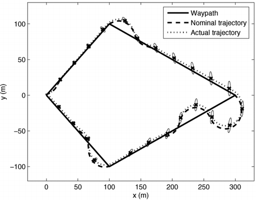
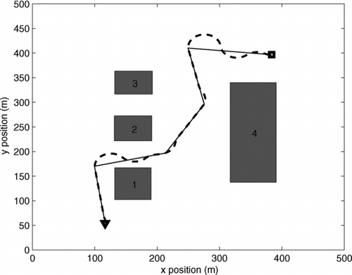
Figure 1 Closed-loop prediction for the waypath following. Uncertainty ellipses are shown in black centred around the actual trajectory

5.3 Offline performance

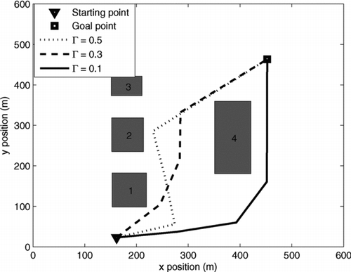
The objective of this subsection is to demonstrate the computational efficiency of the proposed path planning algorithm. We have reported a similar analysis for a linear Gaussian system in Kothari and Postlethwaite (2013); however, that work does not consider a measurement model in the prediction. Here, we evaluate performance of the algorithm for similar scenarios as in Kothari and Postlethwaite (2013). In the first set of simulations, we consider three cases for the scenario shown in Figure 2 with three risks of collision, Γ = 0.5, 0.3 and 0.1. Figure 2 shows the paths and it can be seen that when the risk of collision with any obstacle is reduced, the path moves away from the obstacles to maintain a safe distance.

Figure 2 Paths for different cases using the closed-loop RRT algorithm

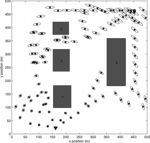
In the second set of simulations, we show the distribution of the nodes during the expansion of the tree for two cases. For the same scenario as in Figure 2 the sample trees are now grown with Γ = 0.5 and 0.1 in Figures 3 and 4, respectively. We can make some key observations. The first observation is that in the first case the tree has nodes closer to the obstacles. This is because we have a less stringent requirement on safety compared to the second case. Second, it can also be seen that there are more uncertainty ellipses in the passage for the first case. We will now show that the algorithm scales up well with the number of obstacles.

Figure 3 Sample tree with Γ = 0.5 generated by the closed-loop RRT algorithm for a simple environment. Each node corresponds to the state distribution mean; a 2 − σ uncertainty ellipse is centred at each node. The mean is shown by ‘x’ in each ellipse

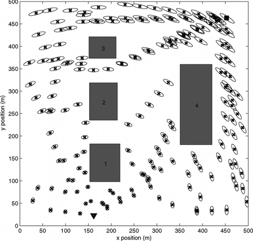
Figure 4 Sample tree with Γ = 0.9 generated by the closed-loop RRT algorithm for a simple environment

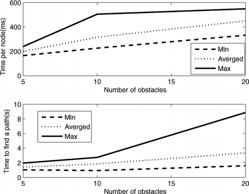
5.3.1 Computational performance

The computational complexity of the closed-loop RRT algorithm mainly depends on the number of obstacles. In this section, we show how the runtime of the proposed algorithm scales with the number of obstacles and we advocate the potential of the algorithm for use in real time. We consider the following six scenarios, with 10 trials performed for each scenario with randomly generated starting and goal locations:

	(1) Five obstacles, closed-loop RRT with Γ = 0.5
	(2) Five obstacles, closed-loop RRT with Γ = 0.1
	(3) Ten obstacles, closed-loop RRT with Γ = 0.5
	(4) Ten obstacles, closed-loop RRT with Γ = 0.1
	(5) Twenty obstacles, closed-loop RRT with Γ = 0.5
	(6) Twenty obstacles, closed-loop RRT with Γ = 0.1

The tree is grown until a probabilistically feasible path is found. Table 1 summarises the minimum, maximum and average runtimes per node and per path, and the same data are plotted in Figure 5. It can be seen from the figure that the minimum and average runtimes increase almost linearly with the number of obstacles, whereas the maximum runtimes show some marked changes. The analysis provides empirical evidence that the computational time needed for the closed-loop RRT scales approximately linearly with the number of obstacles. Hence, the algorithm would appear to be suitable for real-time applications.

Table 3 Simulation results, cluttered environment

		Computational time
		Time per Node (ms)			Time to find a path (s)
Number of				Averaged			Averaged
obstacles	Γ	Minimum	Maximum	over 10 runs	Minimum	Maximum	over 10 runs
5	0.5	165.2	239.1	199.9	0.78	1.66	1.16
5	0.1	173.4	241.5	205.7	1.04	1.96	1.42
10	0.5	119.8	255.9	176.4	0.72	2.19	1.29
10	0.1	234.2	362.5	301.3	0.94	2.73	1.84
20	0.5	332.1	548.7	450.1	1.09	6.75	2.66
20	0.1	400.2	583.1	484.5	1.60	8.86	3.34

Table 1 Tree expansion for each agent

Input: starting condition , initial augmented state , augmented covariance M 0, goal region , time window for tree expansion t a

1: ()

2: while t < t a do

3:  x rand ← RANDOM_VERTEX();

4:   NEAREST_VERTEX(x rand , );

5:  for k = 1 to N do

6:   x extend ← EDGE_EXTEND(, x rand );

7:   x parent ← FIND_PARENT();

8:    Ώ FIND_STATE(x parent );

9:   while is probabilistic feasible and do

10:    u* t ← SELECT_INPUT();

11:    x* t + 1 ← UPDATE_STATE(x* t , u* t );

12:     ← PROPAGATE_STATE();

13:    t ← t+1;

14:   end while

15:   if then

16:    (x extend );

17:    (x extend );

18:    CONNECT_TO_GOAL(x extend );

19:    if x extend is connected to then

20:     Update upper-bound cost-to-go of x extend and its ancestor

21:    end if

22:   end if

23:  end for

24: end while

Figure 5 Computational performance

Remark 1

The path planner works in a decentralised manner and the computational time needed for the closed-loop RRT scales approximately linearly with the number of obstacles as mentioned above. However, if there are many vehicles, they have to communicate to resolve conflicts. In the absence of constraints, the performance of the algorithm does not suffer. But in practice there will be limited bandwidth for communication and therefore the algorithm’s performance may deteriorate for large systems.

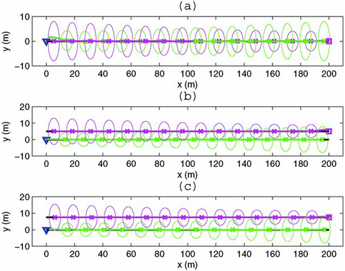
5.3.2 Overlapping probability measure

In this set of simulations, we compute overlapping probabilities for three difference cases where two vehicles are moving ‘towards’ each other with a vertical separation. Figure 6 shows the collision probability corresponding to the cases shown in Figure 7. It can be seen that when the vehicles are at the same level, as shown in Figure 7(a), the probability of collision is higher than when they are not, as in Figure 7(b) and, Figure 7(c), where the distributions are not overlapping significantly. Hence, we can specify a desired safe separation between vehicles by assigning a suitable probability of overlap.

Figure 6 Probability of collision

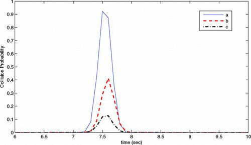
Figure 7 Agents moving towards each other for three different cases

5.4 Online implementation

In this subsection, we show how the tree grows in real time to find a path to a goal location while satisfying probabilistic constraints. The real-time implementation adopts a look-ahead strategy in which the tree is grown during the given time window and then the best branch from the existing tree is chosen for execution. In this example, the sample tree shown in Figure 8(a) is grown for 0.5 sec and a branch is chosen using a heuristic if no path to the goal location is found. The heuristic selects a branch that has the least cost, the cost of the path so far combined with the lower-bound cost-to-go as described in Section 4. The algorithm explores the configuration space to find a complete path or paths with lower cost while tracking the current path. The decision to follow a new path can be made at different time instants based on the time window duration; however, in this example we allow the tree to expand until a vehicle finishes executing the current branch. This is because the vehicle is subject to a turn radius constraint and frequent turning may cause damage to the vehicle. However, the proposed framework allows flexible decision-making to suit the user. Figure 8(b) shows the sample tree after execution of the first waypath. The algorithm finds several paths to the goal location and the minimum cost path is selected for execution. The process of exploration with emphasis on optimisation is continued until the vehicle reaches the goal location. Figure 8(c) and 8(d) show sample trees after executing various waypaths. The searched path and tracked path are shown in Figure 9. It can be seen that the vehicle stays away from the obstacles even during transitions, which are anticipated. Note that during motion the vehicle communicates with neighbouring vehicles, if they are within a communication range, to avoid conflicts. In the next scenario, we show how conflicts can be resolved.

Figure 8 Sample trees

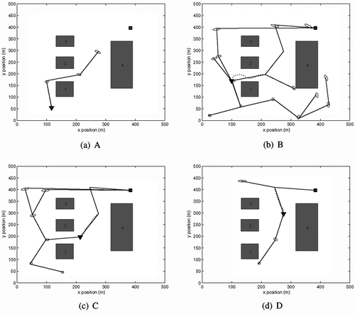
Figure 9 Searched path (solid) and tracked trajectory (dashed)

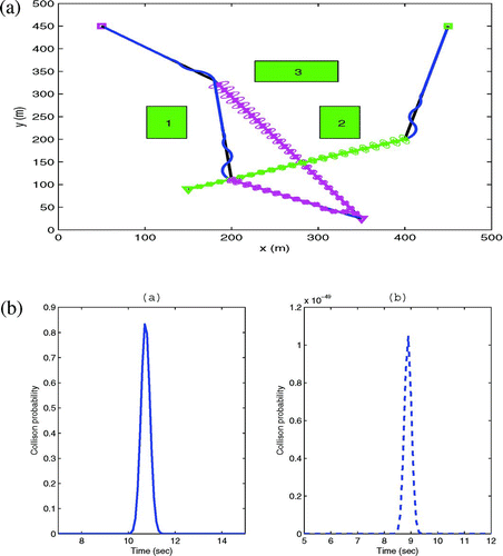
In this set of simulations, we consider the case of two vehicles in conflict. The motion planning scenario is shown in Figure 10(a) for two vehicles. Initially, probabilistically robust paths have been determined for each vehicle without considering the other vehicle in the environment; however, they appear to be in conflict. The conflict is resolved by forcing one vehicle to make a detour. The probability of collision with and without conflict is shown in Figure 10(b). It can be seen when the conflict is resolved the probability of collision is very low (order of 10⁻⁴⁸). This demonstrates the potential of the approach for determining paths while accounting for uncertainties.

Figure 10 An example scenario of conflict resolution in an uncertain dynamic environment. (a) Agents moving towards their goal positions while avoiding conflict. (b) Probability of collision

6. Conclusions

In this paper, we have proposed an algorithm for multi-agent robust path planning in uncertain environments. The path planning process has to deal with two main types of uncertainties: (i) localisation uncertainty due to uncertainty in the initial state and process noise, and (ii) uncertainty in predicting future trajectories from current measurements. In order to take account of these uncertainties we have proposed a method that uses a closed-loop model to predict future information. The closed-loop model derives the most likely measurements and predicts a-priori distributions of the vehicle’s states. Since these distributions are more relevant than open-loop distributions, we have been able to manage the level of uncertainty in the path planning process. Because of this, the planned and executed paths are closer indicating that the planner effectively uses the anticipated information during the planning process.

Also, by introducing the probability constraints, it is possible to manage the feasibility of a solution. We use a chance constraint and the method of overlapping coefficients. The probability of feasibility can be used as a tuning parameter to adjust the level of conservatism in the planning process. Numerical results have been presented to demonstrate the algorithms. In future, the work will be extended to large systems (with many vehicles) where communication can be an issue if agents have to communicate to avoid conflicts. The framework can be further developed for multi-target tracking applications in uncertain environments.

References

- Blackmore , L . “ A probabilistic particle control approach to optimal, robust predictive control ” . In Proceedings of the AIAA Guidance, Navigation and Control Conference. 21–24 August 2006, Keystone, Colorado.
- Blackmore , L. and Ono , M . “ Convex chance constrained predictive control without sampling ” . In Proceedings of the AIAA Guidance, Navigation and Control Conference. 10–13 August 2009, Chicago, Illinois
- Blackmore , L. , Li , H. and Williams , B . “ A probabilistic approach to optimal robust path planning with obstacles ” . In Proceedings of the IEEE American Control Conference. 14–16 June 2006, Minneapolis, Minnesota.
- Du Toit , N. E. and Burdick , J. W. 2011 . Probabilistic collision checking with chance constraints . IEEE Transactions on Robotics , 27 ( 4 ) : 809 – 815 . doi: 10.1109/TRO.2011.2116190
- Frazzoli , E. , Dahleh , M. A. and Feron , E. 2002 . Real-time motion planning for agile autonomous vehicles . AIAA Journal of Guidance, Control, and Dynamics, , 25 ( 1 ) : 116 – 129 . doi: 10.2514/2.4856
- Fulgenzi , C. , Tay , C. , Spalanzani , A. and Laugier , C . “ Probabilistic navigation in dynamic environment using rapidly-exploring random trees and gaussian processes ” . In Proceedings of the IEEE International Conference on Intelligent Robots and Systems 1056 – 1062 .
- Gossner , J. R. , Kouvaritakis , B. and Rossiter , J. A. 1997 . Stable generalized predictive control with constraints and bounded disturbances . Automatica, , 33 ( 4 ) : 551 – 568 . doi: 10.1016/S0005-1098(96)00214-2
- Kewlani , G. , Ishigami , G. and Iagnemma , K . “ Stochastic mobility-based path planning in uncertain environments ” . In Proceedings of the IEEE/RSJ International Conference on Intelligent Robots and Systems IROS 2009 (pp. 1183–1189). 11–15 October 2009, St. Louis
- Kothari , M. and Postlethwaite , I. 2013 . A probabilistically robust path planning algorithm for UAVs using rapidly-exploring random trees . Journal of Intelligent & Robotic Systems, , 71 ( 2 ) : 231 – 253 . doi: 10.1007/s10846-012-9776-4
- Kothari , M. , Postlethwaite , I. and Gu , D. -W . “ Multi-UAV path planning in obstacle rich environments using rapidly-exploring random trees ” . In Proceedings of the 48th IEEE Conference on Decision and Control and 28th Chinese Control Conference. 16–18 December 2009, Shanghai.
- Kuwata , Y. , Richards , A. and How , J. 2007, July . Robust receding horizon control using generalized constraint tightening . Proceedings of the IEEE American Control Conference , : 4482 – 4487 . New York City, NY
- Kuwata , Y. , Teo , J. , Fiore , G. , Karaman , S. , Frazzoli , E. and How , J. P. 2009 . Real-time motion planning with applications to autonomous urban driving . IEEE Transactions on Control Systems Technology, , 17 ( 5 ) : 1105 – 1118 . doi: 10.1109/TCST.2008.2012116
- Lambert , A. , Gruyer , D. and Pierre , G . “ A fast Monte Carlo algorithm for collision probability estimation ” . In Proceedings of the 10th International Conference Control, Automation, Robotics and Vision ICARCV 2008 (pp. 406–411). 17–20 December 2008, Hanoi
- LaValle , S. M. and LaValle , S. M. 2006 . Planning algorithms (pp. 185–246). , Cambridge University Press . ). Sampling-based motion planning. In (Ed.),
- Li , P. , Wendt , M. and Wozny , G. 2002 . A probabilistically constrained model predictive next term controller . Automatica, , 38 ( 7 ) : 1171 – 1176 . doi: 10.1016/S0005-1098(02)00002-X
- Lu , R. , Smith , E. P. and Good , I. J. 1989 . Multivariate measures of similarity and niche overlap . Theoretical Population Biology, , 35 ( 1 ) : 1 – 21 . doi: 10.1016/0040-5809(89)90007-5
- Luders , B. , Kothari , M. and How , J. P . “ Chance constrained RRT for probabilistic robustness to environmental uncertainty ” . In Proceedings of the AIAA Guidance, Navigation, and Control Conference and Exhibit. 2–5 August 2010, Toronto.
- Melchior , N. A. and Simmons , R . “ Particle RRT for path planning with uncertainty ” . In Proceedings of the IEEE International Conference on Robotics and Automation. 10–14 April 2007, Roma.
- Ono , M. and Williams , B. C . “ An efficient motion planning algorithm for stochastic dynamic system with constraints on probability of failure ” . In Proceeding of the 23th AAAI Conference on Artificial Intelligence. Illinois.
- Pepy , R. and Lambert , A . “ Safe path planning in an uncertain-configuration space using RRT ” . In Proceedings of IEEE/RSJ Int Intelligent Robots and Systems Conference, (pp. 5376–5381). 9–15 October 2006, Beijing
- Petersen , K. B. and Pedersen , M. S. Matrix cookbook Retrieved from www.matrixcookbook.com
- Hessem , D. H. 2004 . Stochastic inequality constrained closed-loop model predictive control: with application to chemical process operation (doctoral dissertation). , Delft University Press, Delft .
- Vitus , M. P. and Tomlin , C. J . “ Closed-loop belief space planning for linear, gaussian systems ” . In Proceedings of the IEEE International Robotics and Automation (ICRA) Conference (pp. 2152–2159). 9–13 May 2011, Shanghai
- Yan , Y. and Bitmead , R. R. 2005 . Incorporating state estimation into model predictive control and its application to network traffic control . Automatica, , 41 : 595 – 604 . doi: 10.1016/j.automatica.2004.11.022