Recursive estimation in piecewise affine systems using parameter identifiers and concurrent learning

ABSTRACT

Piecewise affine systems constitute a popular framework for the approximation of non-linear systems and the modelling of hybrid systems. This paper addresses the recursive subsystem estimation in continuous-time piecewise affine systems. Parameter identifiers are extended from continuous-time state-space models to piecewise linear and piecewise affine systems. The convergence rate of the presented identifiers is improved further using concurrent learning, which makes concurrent use of current and recorded measurements. In concurrent learning, assumptions on persistence of excitation are replaced by the less restrictive linear independence of the recorded data. The introduction of memory, however, reduces the tracking ability of concurrent learning because errors in the recorded measurements prevent convergence to the true parameters. In order to overcome this limitation, an algorithm is proposed to detect and remove erroneous measurements at run-time and thereby restore the tracking ability. Detailed examples are included to validate the proposed methods numerically.

KEYWORDS:

• Adaptive systems
• switched systems
• piecewise affine systems
• parameter estimation
• concurrent learning
• outlier detection

1. Introduction

Piecewise affine (PWA) systems constitute a powerful tool to describe complex dynamical systems. They consist of multiple linear subsystems, which define the dynamics of the continuous states. A discrete value indicates the active subsystem. For switched affine systems, this index is an exogenous input signal. For PWA systems, the index is a function of the state and input, and is obtained by partitioning the state-input space of the system. PWA systems have gained popularity due to their universal approximation capabilities for non-linear systems (Azuma, Imura, & Sugie, 2010) and their equivalence to certain hybrid systems (Heemels, Schutter, & Bemporad, 2001).

Identifying PWA systems requires estimating both the linear subsystems as well as the partitions of the state space. This is particularly challenging as available measurements of the state and control input usually do not reveal which subsystem and region they belong to. This is similar to the identification of linear parameter-varying (LPV) systems where the scheduling variable may be unknown (Bamieh & Giarré, 2002; Tóth, 2010; Verdult & Verhaegen, 2002). An overview of identification algorithms for PWA systems is given by Paoletti, Juloski, Ferrari-Trecate, and Vidal (2007). The later survey by Garulli, Paoletti, and Vicino (2012) provides an extensive summary of more recent approaches. The identified models are mostly discrete-time models in input--output form, i.e. switched autoregressive exogenous (SARX) models or piecewise ARX (PWARX) models. However, continuous-time models are more intuitive. Furthermore, as pointed out by Garnier (2015), direct identification of continuous-time models based on sampled data can outperform the discrete-time models in case of rapidly or irregularly sampled data. Algorithms to identify PWA systems in state-space form are less common, due to increased complexity in case the state is not accessible. Exemplary algorithms to deal with discrete-time PWA state-space systems are proposed in Pekpe and Lecœuche (2008), Blackmore, Gil, Seung, and Williams (2007), Bako, Mercère, and Lecoeuche (2009), Bako, Mercère, Vidal, and Lecoeuche (2009), Gil and Williams (2009), Chen, Bako, and Lecoeuche (2011), and Bako, van Luong, Lauer, and Bloch (2013). Identifying state-space systems is considerably more challenging than SARX and PWARX as the partition of the system is based on the state that might not even be measurable. Nevertheless, many control strategies rely on state-space models, which is the first motivation to identify PWA state-space systems. Furthermore, research in realisation theory shows that PWA models in state-space form can realise a greater class of systems than input--output models, i.e. there exist PWA state-space models that cannot be transformed into a corresponding input--output model. Also the conversion from PWA state-space models to PWARX models can result in a tremendous increase of modes and parameters (Garulli et al., 2012). Realisation theory also plays a crucial role in determining, whether a switched system is identifiable or not (Petreczky, 2011; Petreczky & van Schuppen, 2010, 2011). It was shown by Petreczky, Bako, and van Schuppen (2010) that minimality of a realisation is necessary for identifiability. Interestingly, minimality or identifiability of a linear switched system does not imply minimality or identifiability of the linear subsystems.

Most state-of-the-art identification algorithms for PWA systems fall into one of the four major categories: optimisation-based methods, algebraic methods, clustering-based methods or recursive methods. The identification of PWA systems is generally a non-convex combinatorial optimisation problem. The optimisation-based methods seek to solve this problem through a relaxation of the problem (e.g. Bako, 2014; Lauer, Bloch, & Vidal, 2011) or by finding alternative formulations (e.g. Maruta, Sugie, & Kim, 2011). The algebraic methods originate from (Vidal, Soatto, Yi, & Sastry, 2003) and share the idea that multiple ARX models can be identified (independent of the switching sequence) as a single, lifted ARX model. The individual ARX models are retrieved from the lifted model by differentiation. In clustering-based methods, clustering techniques are applied at different stages of the identification process (e.g. Ferrari-Trecate, Muselli, Liberati, & Morari, 2003; Lopes, Borges, & Ishihara, 2013).

Recursive methods, like Bako, Boukharouba, Duviella, and Lecoeuche (2011), Bako et al. (2009), Chen et al. (2011), Vidal (2008), Feiler and Narendra (2008), and Wang and Chen (2011), solve the identification problem online and therefore allow tracking of parameter changes in the system. Also, recursive algorithms handle the available data sequentially and are therefore computationally more efficient. Since the aforementioned properties are desirable, the focus of this article is on recursive estimation algorithms. Some recursive algorithms are modifications of existing batch algorithms: Vidal (2008) for instance extends the original algebraic method in Vidal et al. (2003) to recursively identify SARX systems. Another popular approach is to reason online about the active/best performing model and update the corresponding parameters (Bako et al., 2011; Feiler & Narendra, 2006; Feiler & Narendra, 2008; Wang & Chen, 2011). Proof of convergence remains an open issue for this class of algorithms. Overall, a provably converging, recursive identification algorithm for PWA systems in state-space form is still missing.

The adaptive control literature on the other hand has provably converging algorithms for the control of uncertain PWA systems. The method presented by Di Bernardo, Montanaro, and Santini (2009) allows to identify bimodal piecewise linear (PWL) state-space systems based on the gain evolution of the adaptive controller in Di Bernardo, Montanaro, and Santini (2008). The main drawback of this approach is the limitation to two subsystems. The works by Di Bernardo et al. (2009) and Di Bernardo et al. (2008) show that recursive identification and adaptive control are closely related. In Sang and Tao (2012), exponential tracking is achieved through parameter projection by imposing slow switching and persistence of excitation (PE) on the system. More recently, Di Bernardo, Montanaro, and Santini (2013) proposed a new adaptive control law to asymptotically track the states of a multi-modal PWA reference model. Note that the above adaptive control algorithms for PWA systems share the assumption of known switching hyperplanes. In previous work by Kersting and Buss (2014a, 2014c), adaptive parameter identifiers were extended from linear systems to PWL and PWA systems under the same assumption. Afterwards, they were enhanced in Kersting and Buss (2014b) by the use of concurrent learning.

Chowdhary et al. introduced the concept of concurrent learning to adaptive control in order to circumvent the limitations in adaptive systems related to PE (see Chowdhary, 2010; Chowdhary & Johnson, 2010; Chowdhary, Mühlegg, & Johnson, 2014; Chowdhary, Yucelen, Mühlegg, & Johnson, 2013). While traditional update laws in adaptive control rely on current measurements, the central idea in concurrent learning is to use current measurements concurrently with past measurements. Closely related to concurrent learning is the concept of experience replay, which is applied in reinforcement learning with actor–critic structure (Modares, Lewis, & Naghibi-Sistani, 2014; Wawrzyński, 2009). By replaying recorded past experiences concurrently with current data, convergence rates are improved and assumptions on the excitation of the system are relaxed. The concept of concurrent learning has been applied successfully in various fields (Chowdhary, Mühlegg, How, & Holzapfel, 2013; Kamalapurkar, Walters, & Dixon, 2016; Klotz, Kamalapurkar, & Dixon, 2014). However, the most promising field for concurrent learning is switched systems, where the use of memory enables a continuous adaptation of active and inactive subsystems (De La Torre, Chowdhary, & Johnson, 2013; Kersting & Buss, 2014b). Despite the growing interest in concurrent learning, some of its properties still lack detailed analysis. Especially the effect of erroneous data in the history stacks has received little attention. It is noted by Chowdhary et al. (2013) that tracking errors remain uniformly ultimately bounded and that adaptive weights converge to a compact ball around the ideal weights in the presence of erroneous history stack data. Unfortunately, the size of the compact ball is related to the errors in history stack data. Hence, errors in the history stack limit guaranteed convergence levels.

This paper provides the following contributions. First, we revise the extension of parameter identifiers from linear to PWL/PWA systems and improve the achievable convergence rate using concurrent learning. In addition to previous, preliminary works by Kersting and Buss (2014a, 2014b, 2014c), we provide extended proofs and further insights. Specifically, proving PE for affine systems, which violate the assumption of sufficiently rich input signals, constitutes an enabling contribution for the presented algorithms. Second, we analyse the convergence of concurrent-learning-based parameter identifiers in more detail and propose algorithms to detect and remove erroneous history stack elements online. The extension of Kersting and Buss (2015) to PWA systems is particularly useful due to erroneous stack elements introduced by switching. This not only enables better estimation of the system parameters but also restores the tracking ability of concurrent-learning-based algorithms. Simulation studies illustrate the benefit of concurrent learning and show the approximation of a non-linear hybrid systems.

The remainder of this paper is organised as follows. Section 2 defines parameter identifiers for PWA and PWL systems. The concurrent-learning-based identification of PWA systems is presented in Section 3. The management of history stack data, especially the detection and removal of erroneous data, is subject of Section 4. Section 5 validates the obtained results in numerical simulations of general PWA systems as well as a non-linear hybrid two-tank system. Section 6 concludes the paper.

2. Parameter identifiers for PWA systems

This section defines PWL and PWA systems and discusses briefly how they naturally arise from the linearisation of a non-linear system at multiple operating points. Afterwards, parameter identifiers are extended from linear systems to PWL and PWA systems.

2.1 Definition of PWA systems

PWA systems in state-space form are switched systems of the form (1) $$\begin{array}{c}\hfill \dot{x}\left(t\right)=A_{\sigma \left(t\right)}x\left(t\right)+B_{\sigma \left(t\right)}u\left(t\right)+f_{\sigma \left(t\right)},\end{array}$$(1) where $x\in {\mathbb{R}}^n$, $u\in {\mathbb{R}}^p$ are the state and input vectors, respectively. Let the input u be generated by a stabilising controller such that x and u remain bounded, also for open-loop unstable systems. Let the switched system (1(1) $$\begin{array}{c}\hfill \dot{x}\left(t\right)=A_{\sigma \left(t\right)}x\left(t\right)+B_{\sigma \left(t\right)}u\left(t\right)+f_{\sigma \left(t\right)},\end{array}$$(1) ) consist of $N\in \mathbb{N}$ subsystems, where each subsystem i is characterised by a system matrix $A_i\in {\mathbb{R}}^{n\times n}$, an input matrix $B_i\in {\mathbb{R}}^{n\times p}$ and an affine input vector $f_i\in {\mathbb{R}}^n$. The piecewise constant switching signal σ(t) ∈ {1,… , N} indicates the currently active subsystem.

In PWA systems, σ is a function of the system state x and its input u. The extended state-input space ${\mathbb{R}}^{n+p}$ is partitioned into polyhedral regions Ω _i . In order to form a complete partition ${\cup }_{i=1}^N{\Omega }_i={\mathbb{R}}^{n+p}$, the regions do not overlap, i.e. Ω _i ∩Ω _j = ∅, ∀i ≠ j. The value of the switching signal σ(x(t), u(t)) is given by the index of the region that currently contains the state-input vector: $$\begin{array}{c}\hfill \sigma \left(t\right)=i\text{if}\left[\begin{array}{c}x\left(t\right)\\ u\left(t\right)\end{array}\right]\in {\Omega }_i,i=1,\cdots ,N.\end{array}$$

In order to obtain a well-posed identification problem, it must be possible to excite all states in x for all subsystems. This in turn poses restrictions on the allowed partitions Ω _i . Hence, throughout this article, we assume that all Ω _i are such that they allow sufficient excitation of the state x. For more details on the well-posedness of identification problems for switched systems, refer to Petreczky et al. (2010).

The challenge in identifying PWA systems originates from the coupling between subsystem dynamics (A _i , B _i and f _i ) and the polyhedral regions Ω _i that might both be assumed unknown and thus need to be identified. In Kersting and Buss (2014b) as well as in the remainder of this paper, we consider the simplified case in which the switching signal σ(t) is known. This constitutes on the one hand a restrictive assumption for the identification of PWA systems, as it generally reduces the identification of PWA systems to the identification of N individual subsystems A _i , B _i and f _i . On the other hand, it is in line with adaptive control concepts for PWA systems (Di Bernardo et al., 2008; Di Bernardo et al., 2013; Sang & Tao, 2012). Also, this is acceptable for the second objective of this paper, which is to provide insights into concurrent learning and to extend its capabilities.

A PWA model (1(1) $$\begin{array}{c}\hfill \dot{x}\left(t\right)=A_{\sigma \left(t\right)}x\left(t\right)+B_{\sigma \left(t\right)}u\left(t\right)+f_{\sigma \left(t\right)},\end{array}$$(1) ) can be obtained by linearising a non-linear system around multiple operating points. Consider therefore the non-linear system (2) $$\begin{array}{c}\hfill \dot{x}\left(t\right)=g\left(x\left(t\right),u\left(t\right)\right),\end{array}$$(2) where g is a non-linear vector function of dimension n. Note that for the rest of this paper the time instance t is omitted as long as it is clear from the context. Neglecting higher-order terms in the linearisation of g around an operating point (x* _i , u_i *), the affine model is obtained as (3) $$\begin{array}{ccc}\hfill \dot{x}& =& g(x_i^{*},u_i^{*})+A_i(x-x_i^{*})+B_i(u-u_i^{*})\hfill \\ & =& A_{i}x+B_{i}u+g(x_i^{*},u_i^{*})-A_i{x}_i^{*}-B_i{u}_i^{*}\hfill \\ & =& A_{i}x+B_{i}u+f_i,\hfill \end{array}$$(3) where $A_i=\frac{\partial g(x,u)}{\partial x}{|}_{(x_i^{*},u_i^{*})}$, $B_i=\frac{\partial g(x,u)}{\partial u}{|}_{(x_i^{*},u_i^{*})}$ and f_i = g(x* _i , u* _i ) − A_ix* _i − B_ix* _i . Linearising around various operating points {(x* _i , u_i *)} _{i = 1, …, N} yields a PWA model. In this PWA model, the state space is partitioned such that the linear subsystem in each region is characterised by a minimal error compared to the original non-linear system.

Assuming that (x* _i , u_i *) are known equilibrium points and considering only the deviations Δx_i = x − x* _i and Δu_i = u − u* _i from these equilibrium points, the same considerations yield a PWL model without the affine vectors f _i : $$\begin{array}{c}\hfill \dot{x}=A_i\Delta x_i+B_i\Delta u_i.\end{array}$$Note however that working with PWL models requires the additional knowledge about the equilibrium points in order to compute the deviations Δx _i and Δu _i . Therefore, PWA models are more favourable when it comes to designing adaptive algorithms as less knowledge about the system is required.

The actual partitions Ω _i of a PWA model, approximating a non-linear system, are often unknown in practice. In such cases, one can define a sufficiently large number of fictitious partitions in order to obtain a satisfactory approximation of the actual switching behaviour. The assumption of a known switching signal σ is hence satisfied for such designer-chosen partitions.

With the introduced notation for PWA systems, the problem of estimating the subsystem parameters of a PWA system online is formulated as follows:

Problem 2.1:

Assume that the identification problem is well-posed. Given the partitions Ω _i and hence also the switching signal σ(t), find update laws which are based on the measured state x and input u, and provably drive the dynamic estimates ${\widehat{A}}_i\left(t\right)$, ${\widehat{B}}_i\left(t\right)$ and ${\widehat{f}}_i\left(t\right)$ to the true system parameters A _i , B _i and f _i .

2.2 Parameter identifiers for PWA systems

The literature on adaptive systems offers identifiers to recursively identify the parameters of linear state-space models (see Ioannou & Sun, 1996, Chapter 4). Those identifiers extend to switched affine systems in state-space form by carefully including the switching signal σ. The update laws in parameter identifiers are based on prediction errors. Therefore, the state of the currently active subsystem (σ(t) = i) is predicted with the state observer: (4) $$\begin{array}{c}\hfill {\dot{\widehat{x}}}_i=A_m{\widehat{x}}_i+({\widehat{A}}_i-A_m)x+{\widehat{B}}_{i}u+{\widehat{f}}_i,\text{if}\sigma =i,\end{array}$$(4) where the stable (Hurwitz) design matrix $A_m\in {\mathbb{R}}^{n\times n}$ ensures boundedness of ${\widehat{x}}_i$. Hence, there always exists a symmetric, positive definite $P\in {\mathbb{R}}^{n\times n}$ satisfying (5) $$\begin{array}{c}\hfill A_m^{\top }P+P{A}_m=-Q_e,\end{array}$$(5) with a positive definite matrix $Q_e\in {\mathbb{R}}^{n\times n}$.

Define the prediction error $e_i={\widehat{x}}_i-x$, which provides information about the fit of subsystem i. It is used to update the parameter estimates of the active subsystem. For inactive subsystems e _i is unrelated. The predicted state ${\widehat{x}}_i$ is thus reset and kept equal to the true state x as long as the corresponding subsystem is inactive: (6) $$\begin{array}{c}\hfill {\widehat{x}}_i=x,\text{if}\sigma \ne i.\end{array}$$(6)

Figure 1 shows the state prediction for the ith subsystem with continuous prediction (4(4) $$\begin{array}{c}\hfill {\dot{\widehat{x}}}_i=A_m{\widehat{x}}_i+({\widehat{A}}_i-A_m)x+{\widehat{B}}_{i}u+{\widehat{f}}_i,\text{if}\sigma =i,\end{array}$$(4) ) and state reset (6(6) $$\begin{array}{c}\hfill {\widehat{x}}_i=x,\text{if}\sigma \ne i.\end{array}$$(6) ). This reset is the crucial step in extending parameter identifiers to switched systems because it ensures that switching between different subsystems does not destabilise the overall system.

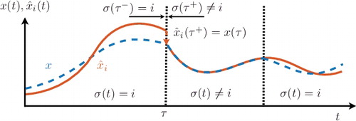
Figure 1. Discrete reset of the state prediction for the ith subsystem upon deactivation of the ith subsystem dynamics, i.e. ${\widehat{x}}_i\left({\tau }^{+}\right)=x\left(\tau \right)$ as σ(τ⁻) = i and σ(τ⁺) ≠ i.

Note that some preliminaries are needed for convergence analysis. Therefore, Appendix A details a definition for PE as well as two useful lemmas from the adaptive control literature (Ioannou & Sun, 1996). It is well known that PE conditions in adaptive systems can be derived from the spectral distribution of input or reference signals. The following definition captures such spectral properties.

Definition 2.1

(sufficiently rich): A signal $u:{\mathbb{R}}^{+}\to \mathbb{R}$ is called sufficiently rich of order 2n, if it consists of at least n distinct frequencies (Ioannou & Sun, 1996, Def. 5.2.1).

The state of the art in parameter identifiers (see Ioannou & Sun, 1996, Chapter 5) requires all input signals of a controllable system to be sufficiently rich of order n + 1. In PWA systems, however, the affine vectors f _i are constant and therefore violate this assumption. Hence, the following lemma is needed for the extension to PWA systems as it ensures PE of the internal signal vector [x ^⊤, u ^⊤, 1]^⊤.

Lemma 2.1:

Consider an affine subsystem (3(3) $$\begin{array}{ccc}\hfill \dot{x}& =& g(x_i^{*},u_i^{*})+A_i(x-x_i^{*})+B_i(u-u_i^{*})\hfill \\ & =& A_{i}x+B_{i}u+g(x_i^{*},u_i^{*})-A_i{x}_i^{*}-B_i{u}_i^{*}\hfill \\ & =& A_{i}x+B_{i}u+f_i,\hfill \end{array}$$(3) ) with controllable pair (A, B) and invertible A. If the input signals in u are sufficiently rich of order n + 1 with distinct frequencies, then the vector z = [x ^⊤, u ^⊤, 1]^⊤ is PE.

The proof of Lemma 2.1 is given in Appendix A for improved readability. Lemma 2.1 extends the state of the art in a sense that violating the common assumption of sufficiently rich input signals can be compensated by restricting the system to invertible system matrices. This insight enables the application of parameter identifiers for PWA systems.

Lemma 2.1 relates PE of each affine subsystem to the richness of the inputs. For the considered class of PWA systems, however, PE should also reflect how frequently each subsystem is visited over time. Only if each subsystem is PE and visited in a persistent manner, it is possible to estimate all system parameters. The first formal but restrictive notion for PE in switched linear systems is given by Petreczky and Bako (2011). In this paper, we require the input signals to be sufficiently rich and such that they repeatedly drive the system through all regions in order to ensure PE of the PWA system.

Theorem 2.1:

Consider the switched system (1(1) $$\begin{array}{c}\hfill \dot{x}\left(t\right)=A_{\sigma \left(t\right)}x\left(t\right)+B_{\sigma \left(t\right)}u\left(t\right)+f_{\sigma \left(t\right)},\end{array}$$(1) ) with controllable pairs (A _i , B _i ) and A _i invertible. Let the state of the system be predicted by Equations (4(4) $$\begin{array}{c}\hfill {\dot{\widehat{x}}}_i=A_m{\widehat{x}}_i+({\widehat{A}}_i-A_m)x+{\widehat{B}}_{i}u+{\widehat{f}}_i,\text{if}\sigma =i,\end{array}$$(4) ) and (6(6) $$\begin{array}{c}\hfill {\widehat{x}}_i=x,\text{if}\sigma \ne i.\end{array}$$(6) ) for all subsystems. If the input signals in u are sufficiently rich of order n + 1 with distinct frequencies, and such that they cause repeated activation of all subsystems obeying a certain dwell time T ₀, then the update laws (7) $$\begin{array}{c}\hfill {\dot{\widehat{A}}}_i^{\text{C}}=-{\Gamma }_{1}P{e}_i{x}^{\top },{\dot{\widehat{B}}}_i^{\text{C}}=-{\Gamma }_{2}P{e}_i{u}^{\top },{\dot{\widehat{f}}}_i^{\text{C}}=-{\Gamma }_{3}P{e}_i,\end{array}$$(7) with P from Equation (5(5) $$\begin{array}{c}\hfill A_m^{\top }P+P{A}_m=-Q_e,\end{array}$$(5) ) and scaling constants ${\Gamma }_1,{\Gamma }_2,{\Gamma }_3\in {\mathbb{R}}^{+}$, cause the estimates ${\widehat{A}}_i,{\widehat{B}}_i,{\widehat{f}}_i$ to converge to the real system matrices A _i , B _i , f _i and cause the prediction errors $e_i={\widehat{x}}_i-x$ to converge to zero.

Proof:

The superscript C in Equation (7(7) $$\begin{array}{c}\hfill {\dot{\widehat{A}}}_i^{\text{C}}=-{\Gamma }_{1}P{e}_i{x}^{\top },{\dot{\widehat{B}}}_i^{\text{C}}=-{\Gamma }_{2}P{e}_i{u}^{\top },{\dot{\widehat{f}}}_i^{\text{C}}=-{\Gamma }_{3}P{e}_i,\end{array}$$(7) ) indicates that the update laws only depend on current measurements. This distinction is important for the later introduction of concurrent learning but is irrelevant for the following proof. The superscript C is thus neglected.

The proof is separated into two parts. In the first part, we show stability of all estimates in the switched system. Multiple Lyapunov functions guarantee stability even for arbitrary fast switching. Note that we apply the same stability notation as Liberzon (2003) throughout the paper, which at the same time serves as an excellent introduction to switched systems. In the second part, we prove convergence to the true parameters with the help of PE. Convergence is achieved under a loose minimal dwell time condition needed to ensure sufficient excitation of the system.

Part I – Stability: In order to formulate a quadratic candidate Lyapunov function for each subsystem in terms of the parameter errors ${\tilde{A}}_i={\widehat{A}}_i-A_i$, ${\tilde{B}}_i={\widehat{B}}_i-B_i$ and ${\tilde{f}}_i={\widehat{f}}_i-f_i$, they are combined in a single column vector (8) $$\begin{array}{c}\hfill {\tilde{\theta }}_i={\left[\begin{array}{ccc}\text{vec}{\left({\tilde{A}}_i\right)}^{\top }& \text{vec}{\left({\tilde{B}}_i\right)}^{\top }& {\tilde{f}}_i^{\top }\end{array}\right]}^{\top }\in {\mathbb{R}}^{n(n+p+1)},\end{array}$$(8) where the vec-operator concatenates the columns of a matrix. We make use of the Kronecker product ⊗ and introduce the matrices (9) $$\begin{array}{c}\hfill \Gamma \triangleq \left[\begin{array}{ccc}{\Gamma }_1{I}_{nn}& 0& 0\\ 0& {\Gamma }_2{I}_{np}& 0\\ 0& 0& {\Gamma }_3{I}_n\end{array}\right],\Psi \triangleq \left[\begin{array}{c}x\\ u\\ 1\end{array}\right]\otimes I_n,\end{array}$$(9) with identity matrices I _n , I _nn and I _np of dimensions n × n, nn × nn and np × np, respectively, which allow expressing most equations in a more compact form, which in turn simplifies the later analysis. The derivative of the prediction error for the active subsystem in terms of ${\tilde{\theta }}_i$ is given by (10) $$\begin{array}{cc}\hfill {\dot{e}}_i& ={\dot{\widehat{x}}}_i-\dot{x}=A_m{e}_i+{\tilde{A}}_{i}x+{\tilde{B}}_{i}u+{\tilde{f}}_i\hfill \\ & =A_m{e}_i+{\Psi }^{\top }{\tilde{\theta }}_i.\hfill \end{array}$$(10) Also, with Equations (8(8) $$\begin{array}{c}\hfill {\tilde{\theta }}_i={\left[\begin{array}{ccc}\text{vec}{\left({\tilde{A}}_i\right)}^{\top }& \text{vec}{\left({\tilde{B}}_i\right)}^{\top }& {\tilde{f}}_i^{\top }\end{array}\right]}^{\top }\in {\mathbb{R}}^{n(n+p+1)},\end{array}$$(8) ) and (9(9) $$\begin{array}{c}\hfill \Gamma \triangleq \left[\begin{array}{ccc}{\Gamma }_1{I}_{nn}& 0& 0\\ 0& {\Gamma }_2{I}_{np}& 0\\ 0& 0& {\Gamma }_3{I}_n\end{array}\right],\Psi \triangleq \left[\begin{array}{c}x\\ u\\ 1\end{array}\right]\otimes I_n,\end{array}$$(9) ), the update laws (7(7) $$\begin{array}{c}\hfill {\dot{\widehat{A}}}_i^{\text{C}}=-{\Gamma }_{1}P{e}_i{x}^{\top },{\dot{\widehat{B}}}_i^{\text{C}}=-{\Gamma }_{2}P{e}_i{u}^{\top },{\dot{\widehat{f}}}_i^{\text{C}}=-{\Gamma }_{3}P{e}_i,\end{array}$$(7) ) take the form (11) $$\begin{array}{c}\hfill {\dot{\tilde{\theta }}}_i={\dot{\widehat{\theta }}}_i^C=-\Gamma \Psi P{e}_i.\end{array}$$(11)

Consider the quadratic candidate Lyapunov function (12) $$\begin{array}{c}\hfill V_i=\left[\begin{array}{cc}{e}_i^{\top }& {\tilde{\theta }}_i^{\top }\end{array}\right]\left[\begin{array}{cc}P& 0\\ 0& {\Gamma }^{-1}\end{array}\right]\left[\begin{array}{c}{e}_i\\ {\tilde{\theta }}_i\end{array}\right].\end{array}$$(12) Its time derivative along Equations (10(10) $$\begin{array}{cc}\hfill {\dot{e}}_i& ={\dot{\widehat{x}}}_i-\dot{x}=A_m{e}_i+{\tilde{A}}_{i}x+{\tilde{B}}_{i}u+{\tilde{f}}_i\hfill \\ & =A_m{e}_i+{\Psi }^{\top }{\tilde{\theta }}_i.\hfill \end{array}$$(10) ) and (11(11) $$\begin{array}{c}\hfill {\dot{\tilde{\theta }}}_i={\dot{\widehat{\theta }}}_i^C=-\Gamma \Psi P{e}_i.\end{array}$$(11) ) yields (13) $$\begin{array}{ccc}\hfill {\dot{V}}_i& =& e_i^{\top }{A}_{\text{m}}^{\top }P{e}_i+e_i^{\top }P{A}_{\text{m}}{e}_i+{\tilde{\theta }}_i^{\top }\Psi P{e}_i+e_i^{\top }P{\Psi }^{\top }{\tilde{\theta }}_i\hfill \\ & & -e_i^{\top }{P}^{\top }{\Psi }^{\top }{\Gamma }^{\top }{\Gamma }^{-1}{\tilde{\theta }}_i-{\tilde{\theta }}_i^{\top }{\Gamma }^{-1}\Gamma \Psi P{e}_i\hfill \\ & =& e_i^{\top }(A_{\text{m}}^{\top }P+P{A}_{\text{m}})e_i=-e_i^{\top }{Q}_e{e}_i,\hfill \end{array}$$(13) for σ = i. For the inactive subsystems, e _i = 0 due to Equation (6(6) $$\begin{array}{c}\hfill {\widehat{x}}_i=x,\text{if}\sigma \ne i.\end{array}$$(6) ). Therefore, the Lyapunov function of the inactive subsystems remains constant, i.e. ${\dot{V}}_i=0$ for σ ≠ i.

While Equation (13(13) $$\begin{array}{ccc}\hfill {\dot{V}}_i& =& e_i^{\top }{A}_{\text{m}}^{\top }P{e}_i+e_i^{\top }P{A}_{\text{m}}{e}_i+{\tilde{\theta }}_i^{\top }\Psi P{e}_i+e_i^{\top }P{\Psi }^{\top }{\tilde{\theta }}_i\hfill \\ & & -e_i^{\top }{P}^{\top }{\Psi }^{\top }{\Gamma }^{\top }{\Gamma }^{-1}{\tilde{\theta }}_i-{\tilde{\theta }}_i^{\top }{\Gamma }^{-1}\Gamma \Psi P{e}_i\hfill \\ & =& e_i^{\top }(A_{\text{m}}^{\top }P+P{A}_{\text{m}})e_i=-e_i^{\top }{Q}_e{e}_i,\hfill \end{array}$$(13) ) shows stability in the sense of Lyapunov for all subsystems individually, it does not imply stability of the overall switched system. In order to prove stability for the obtained hybrid system, we will see that the candidate Lyapunov functions have to be Lyapunov-like functions along all possible trajectories and switching sequences (Branicky, 1998; Liberzon, 2003). This requires the values of the Lyapunov functions at each activation of the corresponding subsystem to form a decreasing sequence.

A precise notation for the switching instances is required in order to show that the candidate Lyapunov functions are Lyapunov-like. Express the qth activation of sub-model i by ${\tau }_{i,q}^{\text{in}}$ (we have ${\sigma }^{-}\left({\tau }_{i,q}^{\text{in}}\right)\ne i$ and ${\sigma }^{+}\left({\tau }_{i,q}^{\text{in}}\right)=i$). Similarly, the instance ${\tau }_{i,q}^{\text{out}}$ refers to the qth exit from sub-model i (${\sigma }^{-}\left({\tau }_{i,q}^{\text{out}}\right)=i$ and ${\sigma }^{+}\left({\tau }_{i,q}^{\text{out}}\right)\ne i$). With this notation, the following requirement arises for stability in the sense of Lyapunov for switched systems (Branicky, 1998): (14) $$\begin{array}{c}\hfill V_i\left({\tau }_{i,q}^{\text{in}}\right)\ge V_i\left({\tau }_{i,q+1}^{\text{in}}\right),\forall q\ge 1.\end{array}$$(14)

Due to the negative semi-definiteness in Equation (13(13) $$\begin{array}{ccc}\hfill {\dot{V}}_i& =& e_i^{\top }{A}_{\text{m}}^{\top }P{e}_i+e_i^{\top }P{A}_{\text{m}}{e}_i+{\tilde{\theta }}_i^{\top }\Psi P{e}_i+e_i^{\top }P{\Psi }^{\top }{\tilde{\theta }}_i\hfill \\ & & -e_i^{\top }{P}^{\top }{\Psi }^{\top }{\Gamma }^{\top }{\Gamma }^{-1}{\tilde{\theta }}_i-{\tilde{\theta }}_i^{\top }{\Gamma }^{-1}\Gamma \Psi P{e}_i\hfill \\ & =& e_i^{\top }(A_{\text{m}}^{\top }P+P{A}_{\text{m}})e_i=-e_i^{\top }{Q}_e{e}_i,\hfill \end{array}$$(13) ), it follows that (15) $$\begin{array}{c}\hfill V_i\left({\tau }_{i,q}^{\text{in}}\right)\ge V_i\left({\tau }_{i,q}^{\text{out}}\right).\end{array}$$(15) Furthermore, the state reset associated with Equation (6(6) $$\begin{array}{c}\hfill {\widehat{x}}_i=x,\text{if}\sigma \ne i.\end{array}$$(6) ) yields e _i (τ) = 0 for the inactive periods $\tau \in ({\tau }_{i,q}^{\text{out}},{\tau }_{i,q+1}^{\text{in}}]$. With e _i = 0, adaptation pauses and the parameter errors remain constant, i.e. ${\tilde{\theta }}_i\left({\tau }_{i,q}^{\text{out}}\right)={\tilde{\theta }}_i\left({\tau }_{i,q+1}^{\text{in}}\right)$. It follows that $$\begin{array}{ccc}\hfill V_i\left({\tau }_{i,q}^{\text{out}}\right)& =& {\left[e_i^{\top }P{e}_i+{\tilde{\theta }}_i^{\top }{\Gamma }^{-1}{\tilde{\theta }}_i\right]}_{{\tau }_{i,q}^{\text{out}}}\ge {\left[{\tilde{\theta }}_i^{\top }{\Gamma }^{-1}{\tilde{\theta }}_i\right]}_{{\tau }_{i,q+1}^{\text{in}}}\hfill \\ & =& V_i\left({\tau }_{i,q+1}^{\text{in}}\right),\hfill \end{array}$$which shows that Equation (14(14) $$\begin{array}{c}\hfill V_i\left({\tau }_{i,q}^{\text{in}}\right)\ge V_i\left({\tau }_{i,q+1}^{\text{in}}\right),\forall q\ge 1.\end{array}$$(14) ) is satisfied. In other words: switching between different subsystems does not cause divergence of the parameter estimates. It remains to be shown that all errors converge to zero.

Part II – Convergence: The proof of convergence relies on Lemma 2.1 and Lemma A.2 in Appendix A. In order to show asymptotic convergence of the switched error system with multiple Lyapunov functions, the sequence in Equation (14(14) $$\begin{array}{c}\hfill V_i\left({\tau }_{i,q}^{\text{in}}\right)\ge V_i\left({\tau }_{i,q+1}^{\text{in}}\right),\forall q\ge 1.\end{array}$$(14) ) must be shown to be strictly decreasing to zero. This will be achieved by showing that the Lyapunov function derivative of the active subsystem is actually negative definite under PE. A certain dwell time is demanded to sufficiently excite each subsystem and ensure that ${\dot{V}}_i<0,\forall {\tilde{\theta }}_i\ne 0$ while σ = i. Therefore, let the dwell time be equal to the constant T ₀ in the definition of PE (see Definition A.1 in Appendix A). The shorter this dwell time, the lower is the level of excitation and the slower do errors converge.

First, the error dynamics are rewritten in the form of Lemma A.2 given in Appendix A: (16) $$\begin{array}{c}\hfill \left[\begin{array}{c}{\dot{e}}_i\\ {\dot{\tilde{\theta }}}_i\end{array}\right]=\left[\begin{array}{cc}{A}_{\text{m}}& {\Psi }^{\top }\left(t\right)\\ -\Gamma \Psi \left(t\right)P& 0\end{array}\right]\left[\begin{array}{c}{e}_i\\ {\tilde{\theta }}_i\end{array}\right],\end{array}$$(16) with Ψ = z⊗I _n . Note that condition (A2(A2) $$\begin{array}{c}\hfill {\dot{P}}_0+A_0^{\top }{P}_0+P_0{A}_0+C_0{C}_0^{\top }\le 0\end{array}$$(A2) ) has been shown in the previous stability proof in form of Equation (13(13) $$\begin{array}{ccc}\hfill {\dot{V}}_i& =& e_i^{\top }{A}_{\text{m}}^{\top }P{e}_i+e_i^{\top }P{A}_{\text{m}}{e}_i+{\tilde{\theta }}_i^{\top }\Psi P{e}_i+e_i^{\top }P{\Psi }^{\top }{\tilde{\theta }}_i\hfill \\ & & -e_i^{\top }{P}^{\top }{\Psi }^{\top }{\Gamma }^{\top }{\Gamma }^{-1}{\tilde{\theta }}_i-{\tilde{\theta }}_i^{\top }{\Gamma }^{-1}\Gamma \Psi P{e}_i\hfill \\ & =& e_i^{\top }(A_{\text{m}}^{\top }P+P{A}_{\text{m}})e_i=-e_i^{\top }{Q}_e{e}_i,\hfill \end{array}$$(13) ), where P ₀ = diag(P, Γ⁻¹). For convergence of e and $\tilde{\theta }$, Lemma A.2 additionally requires the vector $$\begin{array}{c}\hfill z={\left[\begin{array}{ccc}{x}^{\top }& u^{\top }& 1\end{array}\right]}^{\top }\in {\mathbb{R}}^{n+p+1}\end{array}$$to be PE, which is ensured by Lemma 2.1 under the given assumptions. Consequently with Lemma A.2, the equilibrium e _e = 0, ${\tilde{\theta }}_e=0$ of Equation (16(16) $$\begin{array}{c}\hfill \left[\begin{array}{c}{\dot{e}}_i\\ {\dot{\tilde{\theta }}}_i\end{array}\right]=\left[\begin{array}{cc}{A}_{\text{m}}& {\Psi }^{\top }\left(t\right)\\ -\Gamma \Psi \left(t\right)P& 0\end{array}\right]\left[\begin{array}{c}{e}_i\\ {\tilde{\theta }}_i\end{array}\right],\end{array}$$(16) ) is exponentially stable in the large. Hence, the difference $V_i\left({\tau }_{i,q}^{\text{in}}\right)-V_i\left({\tau }_{i,q+1}^{\text{in}}\right)$ is bounded from above by a negative definite function $W_i(e_i\left({\tau }_{i,q}^{\text{in}}\right),{\tilde{\theta }}_i\left({\tau }_{i,q}^{\text{in}}\right))$. As shown in Liberzon (2003, Theorem 3.1), this implies that multiple Lyapunov functions can be used to reason asymptotic stability of the switched system. In other words, the Lyapunov function of the active subsystem is negative definite, which implies that the sequence in Equation (14(14) $$\begin{array}{c}\hfill V_i\left({\tau }_{i,q}^{\text{in}}\right)\ge V_i\left({\tau }_{i,q+1}^{\text{in}}\right),\forall q\ge 1.\end{array}$$(14) ) is strictly decreasing to zero. Including the assumption that each subsystem i is visited in a persistent manner, this means that all prediction errors e _i as well as all parameter errors ${\tilde{\theta }}_i$ converge to zero, i.e. ${\widehat{A}}_i\to A_i$, ${\widehat{B}}_i\to B_i$ and ${\widehat{f}}_i\to f_i,\forall i$ as t → ∞.

2.3 Parameter identifiers for PWL systems

Considering the simpler case of PWL systems (for which f = 0), one notices that Theorem 2.1 holds with one assumption less, i.e. the matrices A _i are not required to be invertible.

Theorem 2.2:

Consider a PWL system with controllable pairs (A _i , B _i ). Let the state of the system be predicted by Equation (4(4) $$\begin{array}{c}\hfill {\dot{\widehat{x}}}_i=A_m{\widehat{x}}_i+({\widehat{A}}_i-A_m)x+{\widehat{B}}_{i}u+{\widehat{f}}_i,\text{if}\sigma =i,\end{array}$$(4) ) with ${\widehat{f}}_i=0$ and Equation (6(6) $$\begin{array}{c}\hfill {\widehat{x}}_i=x,\text{if}\sigma \ne i.\end{array}$$(6) ) for all subsystems. If the input signals in u are sufficiently rich of order n + 1 with distinct frequencies, and such that they cause repeated activation of all subsystems obeying a certain dwell time T ₀, then the update laws ${\dot{\widehat{A}}}_i^C$ and ${\dot{\widehat{B}}}_i^C$ in Equation (7(7) $$\begin{array}{c}\hfill {\dot{\widehat{A}}}_i^{\text{C}}=-{\Gamma }_{1}P{e}_i{x}^{\top },{\dot{\widehat{B}}}_i^{\text{C}}=-{\Gamma }_{2}P{e}_i{u}^{\top },{\dot{\widehat{f}}}_i^{\text{C}}=-{\Gamma }_{3}P{e}_i,\end{array}$$(7) ) cause the estimates ${\widehat{A}}_i,{\widehat{B}}_i$ to converge to the real system matrices A _i , B _i and cause the prediction errors $e_i={\widehat{x}}_i-x$ to converge to zero.

Proof:

The proof of Theorem 2.2 follows the one of Theorem 2.1 and is therefore sketched briefly. First, stability is verified in the same way as before, i.e. with multiple Lyapunov functions which form the decreasing sequence (14(14) $$\begin{array}{c}\hfill V_i\left({\tau }_{i,q}^{\text{in}}\right)\ge V_i\left({\tau }_{i,q+1}^{\text{in}}\right),\forall q\ge 1.\end{array}$$(14) ). In the second part of the proof, which is concerned with convergence, PE now only needs to be guaranteed for the vector z = [x ^⊤, u ^⊤]^⊤. Analysing the proof of Lemma 2.1 in Appendix A shows that this can be guaranteed without restricting A _i to invertible matrices. The remainder of the proof remains unchanged as compared to Theorem 2.1.

Note that Theorem 2.1 and Theorem 2.2 both assume a certain dwell time of the switched system. This dwell time assumption is however not restrictive. It turns out that arbitrary fast switching does not cause divergence of the estimated parameters. But, if little time is spent in a subsystem, the corresponding estimates receive only minor updates, resulting in slow convergence.

The derivation of parameter identifiers for PWA and PWL systems may seem a little technical. An intuitive interpretation of the discussed identifiers for PWA systems is to initialise a separate identifier for each subsystem and apply it during the time frames in which the corresponding subsystem is active. The update laws (7(7) $$\begin{array}{c}\hfill {\dot{\widehat{A}}}_i^{\text{C}}=-{\Gamma }_{1}P{e}_i{x}^{\top },{\dot{\widehat{B}}}_i^{\text{C}}=-{\Gamma }_{2}P{e}_i{u}^{\top },{\dot{\widehat{f}}}_i^{\text{C}}=-{\Gamma }_{3}P{e}_i,\end{array}$$(7) ) suffer three shortcomings: (1) all signals in u must be sufficiently rich of order n + 1 for all time in order to ensure PE; (2) adaptation of subsystem i only takes place while subsystem i is active; (3) convergence is rather slow. These shortcomings can be overcome by introducing memory in the form of concurrent learning as shown by Kersting and Buss (2014b) and as we revise in the following section.

3. Concurrent learning adaptive identification

The update laws in concurrent-learning-based adaptive control and identification consist of two parts. The first part is based on current measurements of states and control inputs (such as the ones presented in the previous section). The second part is based on selected, past measurements that are stored in memory, the so-called history stacks. The update laws thus make concurrent use of current and recorded data. This idea is motivated by the ability to repeatedly employ the recorded data to compute updates for the system parameters, allowing for continued identification of all subsystems. In the case of switched systems, even estimates of currently inactive subsystems can then be further updated. Furthermore, concurrent learning reduces the PE requirements to a limited period of excitation in which the measurements are taken.

Denote with ($x_{i_j}\in {\mathbb{R}}^n$, $u_{i_j}\in {\mathbb{R}}^p$, ${\dot{x}}_{i_j}\in {\mathbb{R}}^n$) the jth triplet that is recorded while subsystem i is active. Let a total of $q\in \mathbb{N}$ such triplets be recorded for each subsystem i. The elements of the triplets are stored in the three history stacks $X_i\triangleq [x_{i_1},x_{i_2},\dots ,x_{i_q}]$, $U_i\triangleq [u_{i_1},u_{i_2},\dots ,u_{i_q}]$ and ${\dot{X}}_i\triangleq [{\dot{x}}_{i_1},{\dot{x}}_{i_2},\dots ,{\dot{x}}_{i_q}]$. For now, let the number of triplets q be fixed and the stack elements $x_{i_j}$, $u_{i_j}$ and ${\dot{x}}_{i_j}$ be constant. Later, this assumption will be discarded without loss of generality. Furthermore, it will be shown how to record new data for the history stacks and when to replace existing data with new data.

Note that in case the derivatives ${\dot{x}}_{i_j}$ cannot be measured directly, techniques such as fixed point smoothing (Jazwinski, 1970; Shumway & Stoffer, 2006; Simon, 2006) can be applied to get an accurate estimate.

Two assumptions on the history stacks arise.

Assumption 3.1:

For each subsystem i, the history stacks X _i and U _i contain elements, such that there exist n + p + 1 linearly independent vectors ${[x_{i_j}^{\top },u_{i_j}^{\top },1]}^{\top }$.

Assumption 3.1 ensures that the recorded data contain enough information for the identification task and hence amounts to a PE-like condition to guarantee negative definiteness of the Lyapunov function in later proofs of convergence. The existence of linearly independent history stack elements for Assumption 3.1 is guaranteed under PE. Note however that PE is by no means necessary for the collection of the history stack elements. The assumption also implies the lower bound n + p + 1 ≤ q for the number of history stack elements. An upper bound is only given by practical considerations in form of limited, available memory.

Assumption 3.2:

The elements of each history stack ${\dot{X}}_i$ fulfil $A_i{x}_{i_j}+B_i{u}_{i_j}+f_i={\dot{x}}_{i_j},\forall j\in \{1,\dots ,q\}$.

Assumption 3.2 requires the recorded derivative ${\dot{x}}_{i_j}$ to match the real derivative $\dot{x}$ at state $x_{i_j}$ and input $u_{i_j}$. As will be shown in Theorem 3.1, one can relax Assumption 3.2 such that estimates of $\dot{x}$ obtained with fixed point smoothing are sufficiently accurate.

For the jth triplet of subsystem i, define ${\epsilon }_{i_j}$ as the error between estimated and recorded derivative of the state: (17) $$\begin{array}{c}\hfill {\epsilon }_{i_j}\left(t\right)\triangleq {\widehat{A}}_i\left(t\right)x_{i_j}+{\widehat{B}}_i\left(t\right)u_{i_j}+{\widehat{f}}_i\left(t\right)-{\dot{x}}_{i_j}.\end{array}$$(17) Note that the history stack elements $x_{i_j}$, $u_{i_j}$ and ${\dot{x}}_{i_j}$ in Equation (17(17) $$\begin{array}{c}\hfill {\epsilon }_{i_j}\left(t\right)\triangleq {\widehat{A}}_i\left(t\right)x_{i_j}+{\widehat{B}}_i\left(t\right)u_{i_j}+{\widehat{f}}_i\left(t\right)-{\dot{x}}_{i_j}.\end{array}$$(17) ) are constant and thus only the time-varying estimates ${\widehat{A}}_i$, ${\widehat{B}}_i$ and ${\widehat{f}}_i$ cause changes in ${\epsilon }_{i_j}$.

In the ideal case, when Assumption 3.2 is satisfied and thus ${\dot{x}}_{i_j}$ is correctly measured, the error ${ϵ}_{i_j}$ vanishes for the true system parameters: $$\begin{array}{c}\hfill {\epsilon }_{i_j}(A_i,B_i,f_i)=A_i{x}_{i_j}+B_i{u}_{i_j}+f_i-{\dot{x}}_{i_j}=0.\end{array}$$In the suboptimal case, when Assumption 3.2 is violated, the measured derivative differs from the true derivative. To model this, let the measured derivative ${\dot{x}}_{i_j}$ equal the true derivative $\dot{x}(x_{i_j},u_{i_j})$ minus an error term ${\delta }_{i_j}\in {\mathbb{R}}^n$: $$\begin{array}{c}\hfill {\epsilon }_{i_j}(A_i,B_i,f_i)=A_i{x}_{i_j}+B_i{u}_{i_j}+f-\underset{{\dot{x}}_{i_j}}{\underbrace{(\dot{x}(x_{i_j},u_{i_j})-{\delta }_{i_j})}}={\delta }_{i_j}.\end{array}$$

Expressing ${\dot{x}}_{i_j}$ in Equation (17(17) $$\begin{array}{c}\hfill {\epsilon }_{i_j}\left(t\right)\triangleq {\widehat{A}}_i\left(t\right)x_{i_j}+{\widehat{B}}_i\left(t\right)u_{i_j}+{\widehat{f}}_i\left(t\right)-{\dot{x}}_{i_j}.\end{array}$$(17) ) in terms of the true system dynamics $\dot{x}(x_{i_j},u_{i_j})=A_i{x}_{i_j}+B_i{u}_{i_j}+f_i$ and the error ${\delta }_{i_j}$ yields (18) $$\begin{array}{cc}\hfill {\epsilon }_{i_j}& =({\widehat{A}}_i-A_i)x_{i_j}+({\widehat{B}}_i-B_i)u_{i_j}+({\widehat{f}}_i-f_i)+{\delta }_{i_j}\hfill \\ & ={\tilde{A}}_i{x}_{i_j}+{\tilde{B}}_i{u}_{i_j}+{\tilde{f}}_i+{\delta }_{i_j}.\hfill \end{array}$$(18)

While Equation (17(17) $$\begin{array}{c}\hfill {\epsilon }_{i_j}\left(t\right)\triangleq {\widehat{A}}_i\left(t\right)x_{i_j}+{\widehat{B}}_i\left(t\right)u_{i_j}+{\widehat{f}}_i\left(t\right)-{\dot{x}}_{i_j}.\end{array}$$(17) ) specifies how to calculate ${\epsilon }_{i_j}$ online, the expression in Equation (18(18) $$\begin{array}{cc}\hfill {\epsilon }_{i_j}& =({\widehat{A}}_i-A_i)x_{i_j}+({\widehat{B}}_i-B_i)u_{i_j}+({\widehat{f}}_i-f_i)+{\delta }_{i_j}\hfill \\ & ={\tilde{A}}_i{x}_{i_j}+{\tilde{B}}_i{u}_{i_j}+{\tilde{f}}_i+{\delta }_{i_j}.\hfill \end{array}$$(18) ) – which cannot be calculated due to the unknown parameter errors – is beneficial in the later convergence analysis. The errors ${\epsilon }_{i_j}$ form a key element in the recorded data-based part (hence superscript R) of the update laws: (19) $$\begin{array}{ccc}& & {\dot{\widehat{A}}}_i^R=-{\Gamma }_1\sum _{j=1}^q{\epsilon }_{i_j}{x}_{i_j}^{\top },{\dot{\widehat{B}}}_i^R=-{\Gamma }_2\sum _{j=1}^q{\epsilon }_{i_j}{u}_{i_j}^{\top },\hfill \\ & & {\dot{\widehat{f}}}_i^R=-{\Gamma }_3\sum _{j=1}^q{\epsilon }_{i_j}.\hfill \end{array}$$(19)

The rationale behind the update laws (19(19) $$\begin{array}{ccc}& & {\dot{\widehat{A}}}_i^R=-{\Gamma }_1\sum _{j=1}^q{\epsilon }_{i_j}{x}_{i_j}^{\top },{\dot{\widehat{B}}}_i^R=-{\Gamma }_2\sum _{j=1}^q{\epsilon }_{i_j}{u}_{i_j}^{\top },\hfill \\ & & {\dot{\widehat{f}}}_i^R=-{\Gamma }_3\sum _{j=1}^q{\epsilon }_{i_j}.\hfill \end{array}$$(19) ) is to ensure exponential parameter convergence in the Lyapunov function (12(12) $$\begin{array}{c}\hfill V_i=\left[\begin{array}{cc}{e}_i^{\top }& {\tilde{\theta }}_i^{\top }\end{array}\right]\left[\begin{array}{cc}P& 0\\ 0& {\Gamma }^{-1}\end{array}\right]\left[\begin{array}{c}{e}_i\\ {\tilde{\theta }}_i\end{array}\right].\end{array}$$(12) ),which will become evident shortly. As Equation (19(19) $$\begin{array}{ccc}& & {\dot{\widehat{A}}}_i^R=-{\Gamma }_1\sum _{j=1}^q{\epsilon }_{i_j}{x}_{i_j}^{\top },{\dot{\widehat{B}}}_i^R=-{\Gamma }_2\sum _{j=1}^q{\epsilon }_{i_j}{u}_{i_j}^{\top },\hfill \\ & & {\dot{\widehat{f}}}_i^R=-{\Gamma }_3\sum _{j=1}^q{\epsilon }_{i_j}.\hfill \end{array}$$(19) ) does not depend on current measurements of u or x, these update laws continuously update the parameter estimates, which enables convergence even for currently inactive subsystems. By combining the current data-based (superscript C) update laws in Equation (7(7) $$\begin{array}{c}\hfill {\dot{\widehat{A}}}_i^{\text{C}}=-{\Gamma }_{1}P{e}_i{x}^{\top },{\dot{\widehat{B}}}_i^{\text{C}}=-{\Gamma }_{2}P{e}_i{u}^{\top },{\dot{\widehat{f}}}_i^{\text{C}}=-{\Gamma }_{3}P{e}_i,\end{array}$$(7) ) and the recorded data-based (superscript R) update laws in Equation (19(19) $$\begin{array}{ccc}& & {\dot{\widehat{A}}}_i^R=-{\Gamma }_1\sum _{j=1}^q{\epsilon }_{i_j}{x}_{i_j}^{\top },{\dot{\widehat{B}}}_i^R=-{\Gamma }_2\sum _{j=1}^q{\epsilon }_{i_j}{u}_{i_j}^{\top },\hfill \\ & & {\dot{\widehat{f}}}_i^R=-{\Gamma }_3\sum _{j=1}^q{\epsilon }_{i_j}.\hfill \end{array}$$(19) ), we obtain the following theorem which specifies concurrent learning adaptive identification of PWA systems.

Theorem 3.1:

Consider the PWA system (1(1) $$\begin{array}{c}\hfill \dot{x}\left(t\right)=A_{\sigma \left(t\right)}x\left(t\right)+B_{\sigma \left(t\right)}u\left(t\right)+f_{\sigma \left(t\right)},\end{array}$$(1) ) with a known switching signal σ and let the subsystem states be predicted by Equations (4(4) $$\begin{array}{c}\hfill {\dot{\widehat{x}}}_i=A_m{\widehat{x}}_i+({\widehat{A}}_i-A_m)x+{\widehat{B}}_{i}u+{\widehat{f}}_i,\text{if}\sigma =i,\end{array}$$(4) ) and (6(6) $$\begin{array}{c}\hfill {\widehat{x}}_i=x,\text{if}\sigma \ne i.\end{array}$$(6) ). Then the update laws (20) $$\begin{array}{ccc}\hfill {\dot{\widehat{A}}}_i& =& {\dot{\widehat{A}}}_i^{\text{C}}+{\dot{\widehat{A}}}_i^{\text{R}},{\dot{\widehat{B}}}_i={\dot{\widehat{B}}}_i^{\text{C}}+{\dot{\widehat{B}}}_i^{\text{R}},{\dot{\widehat{f}}}_i={\dot{\widehat{f}}}_i^{\text{C}}+{\dot{\widehat{f}}}_i^{\text{R}}\hfill \end{array}$$(20) cause the estimates ${\widehat{A}}_i$, ${\widehat{B}}_i$ and ${\widehat{f}}_i$ to

• either converge exponentially to the true parameters A _i , B _i and f _i if Assumptions 3.1 and 3.2 are satisfied,

• or converge to a compact ball around the true parameters in case only Assumption 3.1 holds.

Proof:

The proof of Theorem 3.1 is based on multiple Lyapunov functions, one per subsystem. The derivative of all Lyapunov functions is shown to be negative definite regardless of σ. The parameter estimates of subsystem i therefore converge towards the true parameters whether the ith subsystem is active (σ = i) or inactive (σ ≠ i). It is therefore possible to analyse the stability of each subsystem individually, which is done in the following by neglecting the index i (i.e. A≜A _i or $x_{{}_j}\triangleq x_{i_j}$).

Again, the parameter error vector $\tilde{\theta }$ enables a compact representation of the concurrent learning-based updated laws. First, rewrite Equation (18(18) $$\begin{array}{cc}\hfill {\epsilon }_{i_j}& =({\widehat{A}}_i-A_i)x_{i_j}+({\widehat{B}}_i-B_i)u_{i_j}+({\widehat{f}}_i-f_i)+{\delta }_{i_j}\hfill \\ & ={\tilde{A}}_i{x}_{i_j}+{\tilde{B}}_i{u}_{i_j}+{\tilde{f}}_i+{\delta }_{i_j}.\hfill \end{array}$$(18) ) as (21) $$\begin{array}{c}\hfill {\epsilon }_{{}_j}={\left(\left[\begin{array}{c}{x}_{{}_j}\\ u_{{}_j}\\ 1\end{array}\right]\otimes I_n\right)}^{\top }\tilde{\theta }+{\delta }_{{}_j}.\end{array}$$(21) Then, recall the definitions of Γ and Ψ in Equation (9(9) $$\begin{array}{c}\hfill \Gamma \triangleq \left[\begin{array}{ccc}{\Gamma }_1{I}_{nn}& 0& 0\\ 0& {\Gamma }_2{I}_{np}& 0\\ 0& 0& {\Gamma }_3{I}_n\end{array}\right],\Psi \triangleq \left[\begin{array}{c}x\\ u\\ 1\end{array}\right]\otimes I_n,\end{array}$$(9) ) as well as the compact representation for $\dot{e}$ in Equation (10(10) $$\begin{array}{cc}\hfill {\dot{e}}_i& ={\dot{\widehat{x}}}_i-\dot{x}=A_m{e}_i+{\tilde{A}}_{i}x+{\tilde{B}}_{i}u+{\tilde{f}}_i\hfill \\ & =A_m{e}_i+{\Psi }^{\top }{\tilde{\theta }}_i.\hfill \end{array}$$(10) ): (22) $$\begin{array}{cc}\hfill \dot{e}& =A_{m}e+{\Psi }^{\top }\tilde{\theta }.\hfill \end{array}$$(22) Additionally, define (23) $$\begin{array}{cc}\hfill \Xi & \triangleq \left(\sum _{j=1}^q\left[\begin{array}{c}{x}_{{}_j}\\ u_{{}_j}\\ 1\end{array}\right]\left[\begin{array}{ccc}{x}_{{}_j}^{\top }& u_{{}_j}^{\top }& 1\end{array}\right]\right)\otimes I_n.\hfill \end{array}$$(23) After a few transformations involving Equations (21(21) $$\begin{array}{c}\hfill {\epsilon }_{{}_j}={\left(\left[\begin{array}{c}{x}_{{}_j}\\ u_{{}_j}\\ 1\end{array}\right]\otimes I_n\right)}^{\top }\tilde{\theta }+{\delta }_{{}_j}.\end{array}$$(21) ) and (23(23) $$\begin{array}{cc}\hfill \Xi & \triangleq \left(\sum _{j=1}^q\left[\begin{array}{c}{x}_{{}_j}\\ u_{{}_j}\\ 1\end{array}\right]\left[\begin{array}{ccc}{x}_{{}_j}^{\top }& u_{{}_j}^{\top }& 1\end{array}\right]\right)\otimes I_n.\hfill \end{array}$$(23) ), the update laws in Equation (20(20) $$\begin{array}{ccc}\hfill {\dot{\widehat{A}}}_i& =& {\dot{\widehat{A}}}_i^{\text{C}}+{\dot{\widehat{A}}}_i^{\text{R}},{\dot{\widehat{B}}}_i={\dot{\widehat{B}}}_i^{\text{C}}+{\dot{\widehat{B}}}_i^{\text{R}},{\dot{\widehat{f}}}_i={\dot{\widehat{f}}}_i^{\text{C}}+{\dot{\widehat{f}}}_i^{\text{R}}\hfill \end{array}$$(20) ) take the form (24) $$\begin{array}{c}\hfill \dot{\tilde{\theta }}=\dot{\widehat{\theta }}=-\Gamma \Psi Pe-\Gamma \Xi \tilde{\theta }-\Gamma \underset{\Delta }{\underbrace{\left({\sum }_{j=1}^q\left[\begin{array}{c}{x}_{{}_j}\\ u_{{}_j}\\ 1\end{array}\right]\otimes {\delta }_{{}_j}\right)}}.\end{array}$$(24)

For stability analysis, consider the same quadratic candidate Lyapunov function (12(12) $$\begin{array}{c}\hfill V_i=\left[\begin{array}{cc}{e}_i^{\top }& {\tilde{\theta }}_i^{\top }\end{array}\right]\left[\begin{array}{cc}P& 0\\ 0& {\Gamma }^{-1}\end{array}\right]\left[\begin{array}{c}{e}_i\\ {\tilde{\theta }}_i\end{array}\right].\end{array}$$(12) ) as before. The time derivative of V along Equations (22(22) $$\begin{array}{cc}\hfill \dot{e}& =A_{m}e+{\Psi }^{\top }\tilde{\theta }.\hfill \end{array}$$(22) ) and (24(24) $$\begin{array}{c}\hfill \dot{\tilde{\theta }}=\dot{\widehat{\theta }}=-\Gamma \Psi Pe-\Gamma \Xi \tilde{\theta }-\Gamma \underset{\Delta }{\underbrace{\left({\sum }_{j=1}^q\left[\begin{array}{c}{x}_{{}_j}\\ u_{{}_j}\\ 1\end{array}\right]\otimes {\delta }_{{}_j}\right)}}.\end{array}$$(24) ) yields: (25) $\begin{array}{rl}\dot{V}& =e^{\mathrm{\top }}{A}_{\text{m}}^{\mathrm{\top }}Pe+e^{\mathrm{\top }}P{A}_{\text{m}}e+{\tilde{\theta }}^{\mathrm{\top }}\mathrm{\Psi }Pe+e^{\mathrm{\top }}P{\mathrm{\Psi }}^{\mathrm{\top }}\tilde{\theta }\\ & -\left(e^{\mathrm{\top }}{P}^{\mathrm{\top }}{\mathrm{\Psi }}^{\mathrm{\top }}{\mathrm{\Gamma }}^{\mathrm{\top }}+{\tilde{\theta }}^{\mathrm{\top }}{\mathrm{\Xi }}^{\mathrm{\top }}{\mathrm{\Gamma }}^{\mathrm{\top }}+{\mathrm{\Delta }}^{\mathrm{\top }}{\mathrm{\Gamma }}^{\mathrm{\top }}\right){\mathrm{\Gamma }}^{-1}\tilde{\theta }\\ & -{\tilde{\theta }}^{\mathrm{\top }}{\mathrm{\Gamma }}^{-1}\left(\mathrm{\Gamma }\mathrm{\Psi }Pe+\mathrm{\Gamma }\mathrm{\Xi }\tilde{\theta }+\mathrm{\Gamma }\mathrm{\Delta }\right)\\ & =e^{\mathrm{\top }}(A_{\text{m}}^{\mathrm{\top }}P+P{A}_{\text{m}})e-{\tilde{\theta }}^{\mathrm{\top }}({\mathrm{\Xi }}^{\mathrm{\top }}+\mathrm{\Xi })\tilde{\theta }-2{\mathrm{\Delta }}^{\mathrm{\top }}\tilde{\theta }\\ & =-e^{\mathrm{\top }}{Q}_{e}e-{\tilde{\theta }}^{\mathrm{\top }}{Q}_{\theta }\tilde{\theta }-2{\mathrm{\Delta }}^{\mathrm{\top }}\tilde{\theta },\end{array}$(25) where $Q_e\triangleq -(A_{\text{m}}^{\top }P+P{A}_{\text{m}})$ and Q _θ≜Ξ^⊤ + Ξ. Recall that Q _e was chosen to be positive definite in the design of the current data-based update laws (7(7) $$\begin{array}{c}\hfill {\dot{\widehat{A}}}_i^{\text{C}}=-{\Gamma }_{1}P{e}_i{x}^{\top },{\dot{\widehat{B}}}_i^{\text{C}}=-{\Gamma }_{2}P{e}_i{u}^{\top },{\dot{\widehat{f}}}_i^{\text{C}}=-{\Gamma }_{3}P{e}_i,\end{array}$$(7) ). Also, because of Assumption 3.1, the matrix Ξ and thus Q _θ are positive definite. Note that the useful consequence that $-{\tilde{\theta }}^{\top }{Q}_{\theta }\tilde{\theta }<0,\forall \tilde{\theta }\ne 0$ results from the recorded data-based update laws (19(19) $$\begin{array}{ccc}& & {\dot{\widehat{A}}}_i^R=-{\Gamma }_1\sum _{j=1}^q{\epsilon }_{i_j}{x}_{i_j}^{\top },{\dot{\widehat{B}}}_i^R=-{\Gamma }_2\sum _{j=1}^q{\epsilon }_{i_j}{u}_{i_j}^{\top },\hfill \\ & & {\dot{\widehat{f}}}_i^R=-{\Gamma }_3\sum _{j=1}^q{\epsilon }_{i_j}.\hfill \end{array}$$(19) ) and thus constitutes the motivation behind Equation (19(19) $$\begin{array}{ccc}& & {\dot{\widehat{A}}}_i^R=-{\Gamma }_1\sum _{j=1}^q{\epsilon }_{i_j}{x}_{i_j}^{\top },{\dot{\widehat{B}}}_i^R=-{\Gamma }_2\sum _{j=1}^q{\epsilon }_{i_j}{u}_{i_j}^{\top },\hfill \\ & & {\dot{\widehat{f}}}_i^R=-{\Gamma }_3\sum _{j=1}^q{\epsilon }_{i_j}.\hfill \end{array}$$(19) ). Assuming the ideal case in Equation (25(25) $\begin{array}{rl}\dot{V}& =e^{\mathrm{\top }}{A}_{\text{m}}^{\mathrm{\top }}Pe+e^{\mathrm{\top }}P{A}_{\text{m}}e+{\tilde{\theta }}^{\mathrm{\top }}\mathrm{\Psi }Pe+e^{\mathrm{\top }}P{\mathrm{\Psi }}^{\mathrm{\top }}\tilde{\theta }\\ & -\left(e^{\mathrm{\top }}{P}^{\mathrm{\top }}{\mathrm{\Psi }}^{\mathrm{\top }}{\mathrm{\Gamma }}^{\mathrm{\top }}+{\tilde{\theta }}^{\mathrm{\top }}{\mathrm{\Xi }}^{\mathrm{\top }}{\mathrm{\Gamma }}^{\mathrm{\top }}+{\mathrm{\Delta }}^{\mathrm{\top }}{\mathrm{\Gamma }}^{\mathrm{\top }}\right){\mathrm{\Gamma }}^{-1}\tilde{\theta }\\ & -{\tilde{\theta }}^{\mathrm{\top }}{\mathrm{\Gamma }}^{-1}\left(\mathrm{\Gamma }\mathrm{\Psi }Pe+\mathrm{\Gamma }\mathrm{\Xi }\tilde{\theta }+\mathrm{\Gamma }\mathrm{\Delta }\right)\\ & =e^{\mathrm{\top }}(A_{\text{m}}^{\mathrm{\top }}P+P{A}_{\text{m}})e-{\tilde{\theta }}^{\mathrm{\top }}({\mathrm{\Xi }}^{\mathrm{\top }}+\mathrm{\Xi })\tilde{\theta }-2{\mathrm{\Delta }}^{\mathrm{\top }}\tilde{\theta }\\ & =-e^{\mathrm{\top }}{Q}_{e}e-{\tilde{\theta }}^{\mathrm{\top }}{Q}_{\theta }\tilde{\theta }-2{\mathrm{\Delta }}^{\mathrm{\top }}\tilde{\theta },\end{array}$(25) ), i.e. ${\delta }_{{}_j}=0,\forall j\in \{1,\dots ,q\}$, then the Δ-term vanishes and the derivative of the candidate Lyapunov function is indeed negative definite. Hence, all prediction errors e and parameter errors $\tilde{\theta }$ converge exponentially to zero.

For the suboptimal case, however, in which ${\delta }_{{}_j}\ne 0$, the derivative (25(25) $\begin{array}{rl}\dot{V}& =e^{\mathrm{\top }}{A}_{\text{m}}^{\mathrm{\top }}Pe+e^{\mathrm{\top }}P{A}_{\text{m}}e+{\tilde{\theta }}^{\mathrm{\top }}\mathrm{\Psi }Pe+e^{\mathrm{\top }}P{\mathrm{\Psi }}^{\mathrm{\top }}\tilde{\theta }\\ & -\left(e^{\mathrm{\top }}{P}^{\mathrm{\top }}{\mathrm{\Psi }}^{\mathrm{\top }}{\mathrm{\Gamma }}^{\mathrm{\top }}+{\tilde{\theta }}^{\mathrm{\top }}{\mathrm{\Xi }}^{\mathrm{\top }}{\mathrm{\Gamma }}^{\mathrm{\top }}+{\mathrm{\Delta }}^{\mathrm{\top }}{\mathrm{\Gamma }}^{\mathrm{\top }}\right){\mathrm{\Gamma }}^{-1}\tilde{\theta }\\ & -{\tilde{\theta }}^{\mathrm{\top }}{\mathrm{\Gamma }}^{-1}\left(\mathrm{\Gamma }\mathrm{\Psi }Pe+\mathrm{\Gamma }\mathrm{\Xi }\tilde{\theta }+\mathrm{\Gamma }\mathrm{\Delta }\right)\\ & =e^{\mathrm{\top }}(A_{\text{m}}^{\mathrm{\top }}P+P{A}_{\text{m}})e-{\tilde{\theta }}^{\mathrm{\top }}({\mathrm{\Xi }}^{\mathrm{\top }}+\mathrm{\Xi })\tilde{\theta }-2{\mathrm{\Delta }}^{\mathrm{\top }}\tilde{\theta }\\ & =-e^{\mathrm{\top }}{Q}_{e}e-{\tilde{\theta }}^{\mathrm{\top }}{Q}_{\theta }\tilde{\theta }-2{\mathrm{\Delta }}^{\mathrm{\top }}\tilde{\theta },\end{array}$(25) ) consists of quadratic terms in e and $\tilde{\theta }$ but is also linear in $\tilde{\theta }$. This observation permits a division of the error space ${\left[e^{\top }{\tilde{\theta }}^{\top }\right]}^{\top }\in {\mathbb{R}}^{n(n+p+2)}$ in two sets as exemplified in Figure 2. For some small values of $\tilde{\theta }$ the linear term dominates, which results in a first closed set for which $\dot{V}>0$. The first set is surrounded by a second set in which the quadratic terms outweigh the linear term and $\dot{V}<0$. The outer set with $\dot{V}<0$ guarantees boundedness of e and $\tilde{\theta }$.

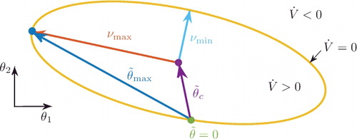
Figure 2. Visualisation of the ellipsoidal set for which $\dot{V}\ge 0$ and approximation of the maximum parameter error $\parallel {\tilde{\theta }}_{max}\parallel$ in terms of the centroid ${\tilde{\theta }}_c$ and the maximal semi-principal axis ν_max of the ellipsoid ($\parallel {\nu }_{max}\parallel =1/\sqrt{{\lambda }_{min}}$).

We can approximate the compact set to which the parameter errors $\tilde{\theta }$ converge by analysing the shape of the boundary between the two sets. On this boundary $\dot{V}=0$, and thus, (26) $$\begin{array}{c}\hfill \left[\begin{array}{cc}{e}^{\top }& {\tilde{\theta }}^{\top }\end{array}\right]\left[\begin{array}{cc}{Q}_e& 0\\ 0& Q_{\theta }\end{array}\right]\left[\begin{array}{c}e\\ \tilde{\theta }\end{array}\right]+\left[\begin{array}{cc}0& 2{\Delta }^{\top }\end{array}\right]\left[\begin{array}{c}e\\ \tilde{\theta }\end{array}\right]=0.\end{array}$$(26)

It is easy to verify that both the origin and the state with e = 0 and $\tilde{\theta }=-2{\left(Q_{\theta }^{-1}\right)}^{\top }\Delta$ reside on this boundary. Furthermore, Equation (26(26) $$\begin{array}{c}\hfill \left[\begin{array}{cc}{e}^{\top }& {\tilde{\theta }}^{\top }\end{array}\right]\left[\begin{array}{cc}{Q}_e& 0\\ 0& Q_{\theta }\end{array}\right]\left[\begin{array}{c}e\\ \tilde{\theta }\end{array}\right]+\left[\begin{array}{cc}0& 2{\Delta }^{\top }\end{array}\right]\left[\begin{array}{c}e\\ \tilde{\theta }\end{array}\right]=0.\end{array}$$(26) ) resembles an ellipsoid in the error space centred at e _c = 0 and ${\tilde{\theta }}_c=-{\left(Q_{\theta }^{-1}\right)}^{\top }\Delta$. An alternative formulation of this ellipsoid is $$\begin{array}{c}\hfill \left[\begin{array}{cc}{e}^{\top }-e_c^{\top }& {\tilde{\theta }}^{\top }-{\tilde{\theta }}_c^{\top }\end{array}\right]\underset{E}{\underbrace{\frac{1}{{\Delta }^{\top }{Q}_{\theta }^{-1}\Delta }\left[\begin{array}{cc}{Q}_e& 0\\ 0& Q_{\theta }\end{array}\right]}}\left[\begin{array}{c}e-e_c\\ \tilde{\theta }-{\tilde{\theta }}_c\end{array}\right]=1.\end{array}$$

The eigenvectors of the positive definite matrix E define the principal axes of the ellipsoid. The length of the semi-axes is given by the square root of the inverse eigenvalues of E. Figure 2 visualises the ellipsoid for a two-dimensional parameter vector θ = [θ₁, θ₂]^⊤.

In a last step, exploiting the triangle inequality on the centroid of the ellipsoid and its maximal semi-principal axis (characterised by the minimal eigenvalue) gives an approximation of the ball around the true parameters to which the estimates converge in the presence of errors ${\delta }_{{}_j}$: $$\begin{array}{c}\hfill \parallel {\tilde{\theta }}_{max}^{*}\parallel \le \parallel {\Delta }^{\top }{Q}_{\theta }^{-1}\parallel +{\left({\lambda }_{min}\left(\frac{Q_{\theta }}{{\Delta }^{\top }{Q}_{\theta }^{-1}\Delta }\right)\right)}^{-\frac{1}{2}},\end{array}$$where ‖ · ‖ is the Euclidean norm and λ_min( · ) denotes the minimum eigenvalue. Compare with Figure 2 for a visual interpretation of this approximation.

While the discussion of concurrent learning thus far involved only PWA systems, it is stressed that the results also apply for PWL systems. In PWL systems, there is no affine input vector f. Consequently, deleting the terms related to f yields the special case of PWL systems. Importantly, this removes the constant 1 in Assumption 3.1 and in the definitions of Ψ and Ξ.

From an adaptive control or identification point of view, the above proof is remarkable in a sense that convergence is guaranteed without the usual PE requirement. The linear independence of the history stack elements (required by Assumption 3.1) replaces PE. This is beneficial as linear independence is considerably easier to monitor than PE. Furthermore, excitation over a limited period of time suffices to record linear independent data.

4. History stack management in concurrent learning

In the discussion of concurrent learning, the stack elements were thus far assumed to be constant. However, looking back at Equation (25(25) $\begin{array}{rl}\dot{V}& =e^{\mathrm{\top }}{A}_{\text{m}}^{\mathrm{\top }}Pe+e^{\mathrm{\top }}P{A}_{\text{m}}e+{\tilde{\theta }}^{\mathrm{\top }}\mathrm{\Psi }Pe+e^{\mathrm{\top }}P{\mathrm{\Psi }}^{\mathrm{\top }}\tilde{\theta }\\ & -\left(e^{\mathrm{\top }}{P}^{\mathrm{\top }}{\mathrm{\Psi }}^{\mathrm{\top }}{\mathrm{\Gamma }}^{\mathrm{\top }}+{\tilde{\theta }}^{\mathrm{\top }}{\mathrm{\Xi }}^{\mathrm{\top }}{\mathrm{\Gamma }}^{\mathrm{\top }}+{\mathrm{\Delta }}^{\mathrm{\top }}{\mathrm{\Gamma }}^{\mathrm{\top }}\right){\mathrm{\Gamma }}^{-1}\tilde{\theta }\\ & -{\tilde{\theta }}^{\mathrm{\top }}{\mathrm{\Gamma }}^{-1}\left(\mathrm{\Gamma }\mathrm{\Psi }Pe+\mathrm{\Gamma }\mathrm{\Xi }\tilde{\theta }+\mathrm{\Gamma }\mathrm{\Delta }\right)\\ & =e^{\mathrm{\top }}(A_{\text{m}}^{\mathrm{\top }}P+P{A}_{\text{m}})e-{\tilde{\theta }}^{\mathrm{\top }}({\mathrm{\Xi }}^{\mathrm{\top }}+\mathrm{\Xi })\tilde{\theta }-2{\mathrm{\Delta }}^{\mathrm{\top }}\tilde{\theta }\\ & =-e^{\mathrm{\top }}{Q}_{e}e-{\tilde{\theta }}^{\mathrm{\top }}{Q}_{\theta }\tilde{\theta }-2{\mathrm{\Delta }}^{\mathrm{\top }}\tilde{\theta },\end{array}$(25) ), one realises that parameter convergence is maintained as long as Q _θ remains positive definite. In other words, as long as Q _θ is ensured to be positive definite, one can arbitrarily replace history stack elements. From a control theoretic perspective, this resembles switching between different stable dynamics that share the common Lyapunov function V. In the following steps, this is exploited in order to further improve the performance of concurrent learning adaptive identification.

4.1 Populating the history stacks

Since initially all history stacks are empty and Assumption 3.1 is violated, consider first the process of populating the history stacks. The history stacks need to be filled with at least n + p + 1 linearly independent elements. Also, a new data point should be sufficiently different from the previously recorded data point. Let Φ(t)≜[x(t)^⊤, u(t)^⊤]^⊤ be the state-input vector at time instance t and let Φ_prev denote the last recorded state-input vector. In concurrent learning, it is common to refer to a new measurement Φ(t) as sufficiently different if the following inequality is satisfied (Chowdhary et al., 2013): (27) $$\begin{array}{c}\hfill \frac{\parallel \Phi \left(t\right)-{\Phi }_{\text{prev}}{\parallel }^2}{\parallel \Phi \left(t\right)\parallel }\ge \upsilon ,\end{array}$$(27) where the threshold $\upsilon \in {\mathbb{R}}^{+}$ is a design parameter. Until the history stack fulfils Assumption 3.1, a new measurement is added to the history stack if x and u are linearly independent of all previously recorded elements and if they fulfil Equation (27(27) $$\begin{array}{c}\hfill \frac{\parallel \Phi \left(t\right)-{\Phi }_{\text{prev}}{\parallel }^2}{\parallel \Phi \left(t\right)\parallel }\ge \upsilon ,\end{array}$$(27) ).

4.2 Maximising the rate of convergence

In order to confine computational complexity, the number of recorded data elements q is limited. Once the history stack is filled with q data points, it has to be reasoned whether replacing old data with new data is beneficial or not.

With the derivative of the Lyapunov function in Equation (25(25) $\begin{array}{rl}\dot{V}& =e^{\mathrm{\top }}{A}_{\text{m}}^{\mathrm{\top }}Pe+e^{\mathrm{\top }}P{A}_{\text{m}}e+{\tilde{\theta }}^{\mathrm{\top }}\mathrm{\Psi }Pe+e^{\mathrm{\top }}P{\mathrm{\Psi }}^{\mathrm{\top }}\tilde{\theta }\\ & -\left(e^{\mathrm{\top }}{P}^{\mathrm{\top }}{\mathrm{\Psi }}^{\mathrm{\top }}{\mathrm{\Gamma }}^{\mathrm{\top }}+{\tilde{\theta }}^{\mathrm{\top }}{\mathrm{\Xi }}^{\mathrm{\top }}{\mathrm{\Gamma }}^{\mathrm{\top }}+{\mathrm{\Delta }}^{\mathrm{\top }}{\mathrm{\Gamma }}^{\mathrm{\top }}\right){\mathrm{\Gamma }}^{-1}\tilde{\theta }\\ & -{\tilde{\theta }}^{\mathrm{\top }}{\mathrm{\Gamma }}^{-1}\left(\mathrm{\Gamma }\mathrm{\Psi }Pe+\mathrm{\Gamma }\mathrm{\Xi }\tilde{\theta }+\mathrm{\Gamma }\mathrm{\Delta }\right)\\ & =e^{\mathrm{\top }}(A_{\text{m}}^{\mathrm{\top }}P+P{A}_{\text{m}})e-{\tilde{\theta }}^{\mathrm{\top }}({\mathrm{\Xi }}^{\mathrm{\top }}+\mathrm{\Xi })\tilde{\theta }-2{\mathrm{\Delta }}^{\mathrm{\top }}\tilde{\theta }\\ & =-e^{\mathrm{\top }}{Q}_{e}e-{\tilde{\theta }}^{\mathrm{\top }}{Q}_{\theta }\tilde{\theta }-2{\mathrm{\Delta }}^{\mathrm{\top }}\tilde{\theta },\end{array}$(25) ), we are able to characterise the rate of convergence. Note that in the ideal case (${\delta }_{i_j}=0$), the derivative of the Lyapunov function of an inactive subsystems (e = 0) is bounded by (28) $$\begin{array}{c}\hfill \dot{V}=-{\tilde{\theta }}^{\top }{Q}_{\theta }\tilde{\theta }\le -{\lambda }_{\text{min}}\left(Q_{\theta }\right){\tilde{\theta }}^{\top }\tilde{\theta }.\end{array}$$(28)

It is thus intuitive to record stack elements $x_{{}_j}$ and $u_{{}_j}$ such that the minimum eigenvalue of Q _θ is maximised, as this maximises the rate of convergence. Especially for full history stacks, this approach allows to reason whether or not it is beneficial to replace an existing stack element with a new measurement. While the same idea is also applied in concurrent learning adaptive identification by Kersting and Buss (2014b), it was Chowdhary et al. (2013) who originally introduced it to concurrent learning adaptive control.

Note that the maximisation of the convergence rate also affects the centroid ${\tilde{\theta }}_c$, which characterises the remaining parameter error. Approximate the squared norm of ${\tilde{\theta }}_c$ as follows: (29) $$\begin{array}{ccc}\hfill \parallel {\tilde{\theta }}_c{\parallel }^2& =& {\Delta }^{\top }{Q}_{\theta }^{-1}{\left(Q_{\theta }^{-1}\right)}^{\top }\Delta \le {\lambda }_{max}^2\left(Q_{\theta }^{-1}\right){\parallel \Delta \parallel }^2\hfill \\ & =& \frac{1}{{\lambda }_{min}^2\left(Q_{\theta }\right)}{\parallel \Delta \parallel }^2.\hfill \end{array}$$(29) According to Equation (29(29) $$\begin{array}{ccc}\hfill \parallel {\tilde{\theta }}_c{\parallel }^2& =& {\Delta }^{\top }{Q}_{\theta }^{-1}{\left(Q_{\theta }^{-1}\right)}^{\top }\Delta \le {\lambda }_{max}^2\left(Q_{\theta }^{-1}\right){\parallel \Delta \parallel }^2\hfill \\ & =& \frac{1}{{\lambda }_{min}^2\left(Q_{\theta }\right)}{\parallel \Delta \parallel }^2.\hfill \end{array}$$(29) ), improving the convergence rate by maximising λ_min(Q _θ) provides a second benefit. That is, with increased λ_min(Q _θ), the error term Δ – caused by errors ${\delta }_{{}_j}$ in the estimation of $\dot{x}(x_{{}_j},u_{{}_j})$ – has a weakened effect on the parameter errors.

4.3 Detecting erroneous history stack elements

Section 3 explained that wrongly recorded or estimated stack elements hinder convergence to the true parameters. This problem has received limited attention in previous works on concurrent learning, excluding De La Torre et al. (2013). Therefore, concurrent learning is expected to work well in case of constant system parameters. However, if system parameters change over time (e.g. due to ageing or wear), then history stack elements become outdated and estimates converge to (or are stuck at) wrong values.

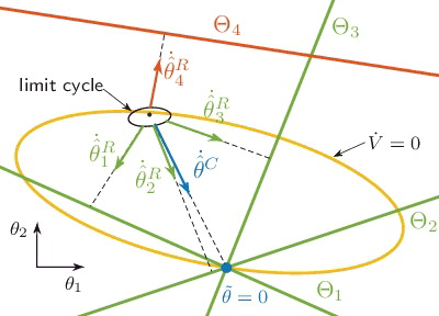
Here we describe the first algorithm to detect and remove erroneous stack elements online (Kersting & Buss, 2015), which is based on the result of Section 3: i.e. estimated parameters converge to an ellipsoidal set in the parameter space (depicted in Figure 2) in the presence of erroneous history stack elements.

In order to understand the cause of this ellipsoid, note that each triplet ($x_j,u_j,{\dot{x}}_j$) in the history stack spans a subspace Θ _j in the parameter space. The subspace Θ _j , associated with the jth triplet, contains all parameter configurations that cannot be falsified by the measurements $(x_j,u_j,{\dot{x}}_j)$, i.e. (30) $$\begin{array}{c}\hfill {\Theta }_j=\{\widehat{\theta }\in {\mathbb{R}}^{n(n+p+1)}|\widehat{A}\left(\widehat{\theta }\right)x_j+\widehat{B}\left(\widehat{\theta }\right)u_j+\widehat{f}\left(\widehat{\theta }\right)={\dot{x}}_j\}.\end{array}$$(30) The parameter configurations $\widehat{\theta }\in {\Theta }_j$ form the solution of an under-determined system of equations, from which the dimension of Θ _j can be found to be $dim\left({\Theta }_j\right)=dim\left(\theta \right)-n=n(n+p)$.

In the error-less case (δ _j = 0, ∀j) and under Assumption 3.1, all subspaces intersect at a single point θ = ∪ ^q _{j = 1}Θ _j , for which $\tilde{\theta }=0$. In case δ _j ≠ 0, however, the subspaces do not intersect at a single point. Figure 3 displays an example with four subspaces. The first three subspaces represent the subspaces of error-less history stack triplets. The fourth subspace corresponds to an erroneous history stack element, which is therefore shifted away from the intersection point. Due to the shifted subspace Θ₄, the estimates do not converge to the true parameter configuration θ. Instead the estimates enter a limit cycle in the ellipsoidal set as shown in the proof of Theorem 3.1. In turn, the prediction error does not converge to zero, i.e. e ≠ 0 or greater than some threshold in the presence of noise.

Figure 3. Exemplary limit cycle in a two-dimensional parameter space. The history stack has four elements for which only δ₄ ≠ 0. The update vectors ${\dot{\widehat{\theta }}}_j^R$ are an orthogonal projection onto Θ _j .

The strategy to detect erroneous history stack elements is to compare the individual contributions in the update laws (20(20) $$\begin{array}{ccc}\hfill {\dot{\widehat{A}}}_i& =& {\dot{\widehat{A}}}_i^{\text{C}}+{\dot{\widehat{A}}}_i^{\text{R}},{\dot{\widehat{B}}}_i={\dot{\widehat{B}}}_i^{\text{C}}+{\dot{\widehat{B}}}_i^{\text{R}},{\dot{\widehat{f}}}_i={\dot{\widehat{f}}}_i^{\text{C}}+{\dot{\widehat{f}}}_i^{\text{R}}\hfill \end{array}$$(20) ). Hence, let the contribution of the current measurements and of the jth history stack triplet be denoted by (31) $$\begin{array}{cc}\hfill {\dot{\widehat{\theta }}}^C(x\left(t\right),u\left(t\right))& =-\Gamma \Psi Pe\hfill \end{array}$$(31) (32) $$\begin{array}{cc}\hfill {\dot{\widehat{\theta }}}_j^R(x_j,u_j,{\dot{x}}_j)& =-\Gamma {\Xi }_j\widehat{\theta }+\Gamma {\xi }_j,j\in \{1,\dots ,q\},\hfill \end{array}$$(32) where $$\begin{array}{c}\hfill {\Xi }_j\triangleq \left(\left[\begin{array}{c}{x}_j\\ u_j\\ 1\end{array}\right]\left[\begin{array}{ccc}{x}_j^{\top }& u_j^{\top }& 1\end{array}\right]\right)\otimes I_n,{\xi }_j\triangleq \left[\begin{array}{c}{x}_j\\ u_j\\ 1\end{array}\right]\otimes {\dot{x}}_j,\end{array}$$which combined in $\dot{\widehat{\theta }}={\dot{\widehat{\theta }}}^C+{\sum }_{j=1}^q{\dot{\widehat{\theta }}}_j^R$ form the original update laws (20(20) $$\begin{array}{ccc}\hfill {\dot{\widehat{A}}}_i& =& {\dot{\widehat{A}}}_i^{\text{C}}+{\dot{\widehat{A}}}_i^{\text{R}},{\dot{\widehat{B}}}_i={\dot{\widehat{B}}}_i^{\text{C}}+{\dot{\widehat{B}}}_i^{\text{R}},{\dot{\widehat{f}}}_i={\dot{\widehat{f}}}_i^{\text{C}}+{\dot{\widehat{f}}}_i^{\text{R}}\hfill \end{array}$$(20) ).

Next, note that the recorded data-based update laws (32(32) $$\begin{array}{cc}\hfill {\dot{\widehat{\theta }}}_j^R(x_j,u_j,{\dot{x}}_j)& =-\Gamma {\Xi }_j\widehat{\theta }+\Gamma {\xi }_j,j\in \{1,\dots ,q\},\hfill \end{array}$$(32) ) correspond to an orthogonal projection onto the subspaces Θ _j . For correct history stack triplets, this projection points into the ellipsoid. Also the current data-based update (31(31) $$\begin{array}{cc}\hfill {\dot{\widehat{\theta }}}^C(x\left(t\right),u\left(t\right))& =-\Gamma \Psi Pe\hfill \end{array}$$(31) ) drives the estimates towards the true parameter configuration under the assumption of persistent excitation. Therefore, ${\dot{\widehat{\theta }}}^C$ serves as a reference point. Convergence is prevented if at least one erroneous stack element exists and points out of the ellipsoid. Therefore, the directional information compared to the current data-based update law is used to reason about the erroneous history stack elements.

Note that the PE requirement for the reference point ${\dot{\widehat{\theta }}}^C$ should not be understood as a limitation at this point. Once the history stack is known to contain erroneous elements, one must in any case record new measurements. In order to fulfil Assumption 3.1, excitation of the system is beneficial. During the collection of new measurements, it can be reasoned which elements are erroneous and need to be replaced. While the existence of measurements, which satisfy Assumption 3.1, is guaranteed under PE, it is not a necessary condition. Future work could analyse how the following ideas perform without PE. As shown in the proof of Theorem 2.1, PE can be ensured by choosing input signals sufficiently rich of order n + 1 with distinct frequencies.

In order to analyse to which extent the recorded data-based update laws (32(32) $$\begin{array}{cc}\hfill {\dot{\widehat{\theta }}}_j^R(x_j,u_j,{\dot{x}}_j)& =-\Gamma {\Xi }_j\widehat{\theta }+\Gamma {\xi }_j,j\in \{1,\dots ,q\},\hfill \end{array}$$(32) ) coincide with the reference vector ${\dot{\widehat{\theta }}}^C$, define for each stack element j the angle ϕ _j between ${\dot{\widehat{\theta }}}^C$ and ${\dot{\widehat{\theta }}}_j^R$: (33) $$\begin{array}{c}\hfill {\varphi }_j\left(t\right)=\sphericalangle \left({\dot{\widehat{\theta }}}^C\left(t\right),{\dot{\widehat{\theta }}}_j^R\left(t\right)\right).\end{array}$$(33)

Note that statements, which are based on the angles ϕ _j , are only meaningful if the norms of the corresponding vectors are sufficiently large. Therefore, we introduce the two thresholds ϑ ^C and ϑ ^R for ${\dot{\widehat{\theta }}}^C$ and ${\dot{\widehat{\theta }}}^R$, respectively. If $\parallel {\dot{\widehat{\theta }}}^C\parallel <{\vartheta }^C$, the current data-based update vector fails to qualify as a reliable reference point. This is for instance the case if the parameter estimates are in the vicinity of the true parameters. For $\parallel {\dot{\widehat{\theta }}}_j^R\parallel <{\vartheta }^R$, the contribution of the jth history stack element is very small. In this case, the jth history stack triplet $(x_j,u_j,{\dot{x}}_j)$ cannot be falsified by the current estimates $\widehat{\theta }$. In summary, falling below these two thresholds corresponds to good estimates. The angle ϕ _j is therefore set to zero whenever one of the two thresholds is not exceeded: (34) $$\begin{array}{c}\hfill {\varphi }_j\left(t\right)\Leftarrow 0,\text{if}\left(\parallel {\dot{\widehat{\theta }}}^C\parallel <{\vartheta }^C\text{or}\parallel {\dot{\widehat{\theta }}}_j^R\parallel <{\vartheta }^R\right).\end{array}$$(34)

The parameter estimates $\widehat{\theta }$ and angles ϕ _j are time-varying for sinusoidal excitation and enter into a limit cycle. Due to the known excitation u, the frequency of this limit cycle can be approximated. Since we are interested in the update directions on average, consider the low-pass filtered angles ${\bar{\varphi }}_j$, where the cut-off frequency of the filter is lower than the lowest excitation frequency in u. The following algorithm to detect and remove erroneous history stack elements is based on the filtered angles ${\bar{\varphi }}_j$.

Algorithm 1:

Consider the concurrent learning-based update law in Theorem 3.1 with errors δ _j . Monitor the filtered angles ${\bar{\varphi }}_j$ according to Equations (33(33) $$\begin{array}{c}\hfill {\varphi }_j\left(t\right)=\sphericalangle \left({\dot{\widehat{\theta }}}^C\left(t\right),{\dot{\widehat{\theta }}}_j^R\left(t\right)\right).\end{array}$$(33) ) and (34(34) $$\begin{array}{c}\hfill {\varphi }_j\left(t\right)\Leftarrow 0,\text{if}\left(\parallel {\dot{\widehat{\theta }}}^C\parallel <{\vartheta }^C\text{or}\parallel {\dot{\widehat{\theta }}}_j^R\parallel <{\vartheta }^R\right).\end{array}$$(34) ). If the parameter estimates enter a limit cycle (i.e. e ≠ 0 and ${\dot{\bar{\varphi }}}_j\approx 0$), replace the kth history stack triplet, where (35) $$\begin{array}{c}\hfill k=arg\underset{j}{max}\left\{{\bar{\varphi }}_j|{\bar{\varphi }}_j\ge \frac{\pi }{2}\right\},\end{array}$$(35) by a new measurement with ${\bar{\varphi }}_{new}<{\bar{\varphi }}_k$ in order to reduce the errors in the history stack.

Since PE constitutes a critical assumption in adaptive systems, we want to complete the theoretical part of this paper by briefly repeating the role of PE in the presented algorithms. For the parameter identifiers discussed in Theorems 2.1 and 2.2, PE is a necessary condition for parameter convergence. The concurrent learning-based parameter identifiers in Theorem 3.1 replace PE by linear independence of the history stack elements. While PE in this context guarantees the existence of linearly independent measurements, PE is by no means necessary in order to obtain them. In case of an erroneous history stack element, we propose in Algorithm 1 to resume PE over a limited period of time in order to detect and replace the erroneous element. Once the erroneous element is replaced, convergence can proceed without PE.

5. Numerical validation

In this section, we numerically validate the proposed update laws for PWA systems as well as Algorithm 1 for the detection of erroneous history stack elements in concurrent learning. First, the advantage of concurrent learning over traditional adaptation is demonstrated for a linear bimodal system. Then, we analyse the estimation and tracking of time-varying parameters with concurrent learning-based parameter identifiers. Afterwards, we compare the proposed algorithm with Recursive Least Squares and with an alternative approach to enable tracking in concurrent learning (De La Torre et al., 2013). Finally, we apply concurrent learning for the adaptive identification of a hybrid two-tank system.

5.1 Benefit of concurrent learning

First, consider a bimodal PWL system with n = 1 and p = 1. Let the parameters for the two subsystems be $$\begin{array}{cccc}\hfill {\theta }_1& ={\left[\begin{array}{cc}-2& 1\end{array}\right]}^{\top }\hfill & \hfill {\Omega }_1& =\{x\in \mathbb{R}|x\ge 0\}\hfill \\ \hfill {\theta }_2& ={\left[\begin{array}{cc}-5& 2\end{array}\right]}^{\top }\hfill & \hfill {\Omega }_2& =\{x\in \mathbb{R}|x<0\}.\hfill \end{array}$$The initial state is x = 1 and the control input is an exponentially decaying sinusoidal signal: u(t) = 5e^−0.1t sin (t). The state derivatives are estimated with fixed point smoothing.

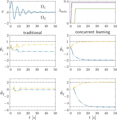
Simulation results with and without concurrent learning are shown in Figure 4 for the design parameters −A _m = P = Γ₁ = Γ₂ = 1. The exponentially decaying state does not yield a persistent excitation of the system. Hence, the estimates do not converge under the traditional update laws. For concurrent learning, the initial excitation is sufficient to fill the history stacks with linear independent data, which can be seen from the increase in λ_min. Based on the recorded data, exponential convergence is achieved for both active (solid lines) and inactive (dotted lines) subsystems. This comparison demonstrates the benefit of concurrent learning in terms of reduced PE requirements and increased convergence rates.

Figure 4. Comparison of parameter identifiers without (left column) and with (right column) concurrent learning. The top left shows the exponentially decaying excitation of the state in both cases. The top right shows the minimum eigenvalues associated with the two history stacks for the concurrent-learning-based estimation.

5.2 Parameter estimation and tracking

First, on a time interval t ∈ [0, 700) s, consider the following PWA system (n = 2, p = 1), which consists of three subsystems with the unknown parameter vectors $$\begin{array}{cc}\hfill {\theta }_1^{\text{'}}& ={\left[\begin{array}{cccccccc}0& -2& 1& -3& 0& 1& 0& 0\end{array}\right]}^{\top }\hfill \\ \hfill {\theta }_2^{\text{'}}& ={\left[\begin{array}{cccccccc}0& -2& 1& -4& 0& 1& 0& 0\end{array}\right]}^{\top }\hfill \\ \hfill {\theta }_3^{\text{'}}& ={\left[\begin{array}{cccccccc}0& -2& 1& -2& 0& 1& 0& 0\end{array}\right]}^{\top }\hfill \end{array}$$and the known state-space partitions $$\begin{array}{cc}\hfill {\Omega }_1& =\left\{x\in {\mathbb{R}}^2:-3\le x_1\le 3\right\}\hfill \\ \hfill {\Omega }_2& =\left\{x\in {\mathbb{R}}^2:x_1<-3\right\}\hfill \\ \hfill {\Omega }_3& =\left\{x\in {\mathbb{R}}^2:x_1>3\right\}.\hfill \end{array}$$To test the tracking abilities, the subsystems abruptly change their parameters at time instance t = 700 s. During the second interval t ∈ [700, 1400) s, the parameters are $$\begin{array}{cc}\hfill {\theta }_1^{\text{'}\text{'}}& ={\left[\begin{array}{cccccccc}0& -3& 1& -1& 0& 1.3& 0& 0.3\end{array}\right]}^{\top }\hfill \\ \hfill {\theta }_2^{\text{'}\text{'}}& ={\left[\begin{array}{cccccccc}0& -2& 1& -2& 0& 1.5& 0& 0.4\end{array}\right]}^{\top }\hfill \\ \hfill {\theta }_3^{\text{'}\text{'}}& ={\left[\begin{array}{cccccccc}0& -3& 1& -2& 0& 1.7& 0& -0.2\end{array}\right]}^{\top }.\hfill \end{array}$$

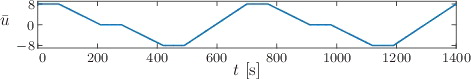
The system is excited with $u\left(t\right)=sin(0.8t)+sin\left(t\right)+sin\left(3t\right)+\bar{u}\left(t\right)$, where $\bar{u}\left(t\right)$ is a ramp-like offset shown in Figure 5, which drives the system into all regions. Therefore, the input signal u is sufficiently rich of order 6, which enables traditional updating according to Theorem 2.1 as well as recording linearly independent data according to Theorem 3.1. Gaussian white noise with zero mean and 10⁻³ variance is added to the state measurement x.

Figure 5. Offset $\bar{u}\left(t\right)$ in the input signal u(t).

The scaling constants are ${\Gamma }_1={\Gamma }_2={\Gamma }_3=1$ for balanced adaptation of A _i , B _i and f _i . For unknown system parameters, we choose the design parameters P = I ₂ and $A_m=-10I_2$. All parameter estimates ${\widehat{\theta }}_i$ are initially zero and the history stacks of size q = 4 are initially empty. Selected estimates of the state derivative for the history stacks are obtained with fixed point smoothing. The design parameters for the detection of erroneous history stack elements are ϑ ^C = 0.09, ${\vartheta }^R\left(t\right)=0.1{max}_j(\parallel {\dot{\widehat{\theta }}}_j^R\left(t\right)\parallel )$.

Figure 6 shows the evolution of estimates ${\widehat{\theta }}_i$ for all subsystems i = 1, 2, 3 on the entire time interval [0, 1400] s. The figure shows that once a subsystem is activated for the first time, its history stacks are quickly filled with measurements and the parameter estimates converge to the true parameters. Note that the transition between two regions is characterised by multiple switches due to the sinusoidal excitation. These switches likely cause the smoothing process to result in erroneous history stack elements. Especially the estimates ${\widehat{\theta }}_3$ converge to wrong parameters between 400 and 450 s. The proposed detection algorithm, however, detects and removes these erroneous elements once the system remains in Ω₃ for a sufficiently long time.

Figure 6. Identification and tracking of PWA subsystem parameters with concurrent-learning-based parameter identifiers and removal of erroneous history stack elements.

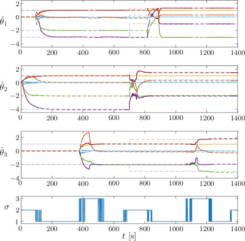
The evolution of ${\widehat{\theta }}_2$ after the parameter change at 700 s shows that the system enters into a limit cycle due to the parameter mismatch. This can be seen by oscillating estimates, which naturally triggers the proposed detection algorithm. In turn, outdated history stack elements taken before the change are successfully replaced. As can also be seen from the figure, the removal of erroneous history stack elements only takes place for the active subsystem, which is why ${\widehat{\theta }}_3$ reacts to the parameter change with a delay of 400 s. Approximately 100 s after a subsystem is activated, the corresponding history stacks do not contain outdated measurements taken with θ′ _i anymore and the estimates converge to the true parameters θ′′ _i .

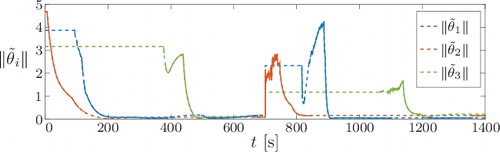
Figure 7 shows the normed parameter errors $\parallel {\tilde{\theta }}_i\parallel$ for all subsystems. At around 400 and 900 s, it can be seen that the sequential removal of erroneous history stack elements according to Algorithm 1 might lead to a temporary increase in the parameter errors. As shown in the proof of Theorem 3.1, however, all errors remain bounded.

Figure 7. Normed parameter errors during concurrent-learning-based parameter estimation with removal of erroneous history stack elements. The lines are dashed for inactive and solid for active subsystems.

5.3 Comparison with cyclic replacement and recursive least squares

Reducing the parameter error $\tilde{\theta }$ in the presence of errors δ _j constitutes a major advantage of the proposed algorithm over other approaches. In this section, we demonstrate this by comparing our approach with the cyclic replacement approach proposed by De La Torre et al. (2013) and recursive least squares (RLS) (see Ljung, 1987, Chapter 11) applied to an affine linear time-invariant (LTI) system. In De La Torre et al. (2013), the ageing of data is modelled with an exponential decay (e ^−0.01t ) on the current history stack. Once a new history stack outperforms the current history stack, the entire history stack is replaced. For the following comparison, the standard RLS algorithm was implemented on the history stack measurements x _j , u _j and ${\dot{x}}_j$ with a forgetting factor γ = 0.95.

A stable, randomly chosen state-space system of higher order (n = 5, p = 2) is considered, i.e. $\theta \in {\mathbb{R}}^{40}$. The system is excited with input signals $u_1\left(t\right)=sin\left(\frac{5}{3}t\right)+cos(1.1t)+sin(1.7t)$ and $u_2\left(t\right)=sin\left(\frac{4}{3}t\right)+cos\left(t\right)+sin\left(\frac{7}{3}t\right)$, each sufficiently rich of order 6 with distinct frequencies. We initialise the history stacks with q = 10 measurements. The errors of each stack element are drawn from a normal distribution ${\delta }_j\sim \mathcal{N}(0,0.3)$. For 2000 s, the stack elements with the greatest errors (detected by the mechanism according to Algorithm 1) are replaced by new measurements. Note that the errors δ _j of new elements follow the same normal distribution as the initial errors. The chosen design parameters are the same as in Section 5.2.

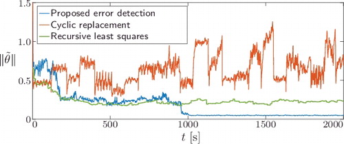
Figure 8 shows the estimation process in terms of the normed parameter errors for all three approaches. The normed parameter error for the cyclic replacement approach is greater than the normed error obtained with our error detection approach, because the cyclic replacement exchanges the entire history stack at once. In that case, it is likely that the history stack contains elements with similarly large errors, leading to no improvement. Even though RLS provides lower estimation errors than concurrent learning with cyclic replacement, it is still affected by the errors δ _j . In contrast, the algorithm proposed here selectively replaces the most erroneous history stack element. After about 900 s, the algorithm has found history stack elements with sufficiently small errors which cause the update terms to fall below the thresholds ϑ ^C and ϑ ^R in Equation (34(34) $$\begin{array}{c}\hfill {\varphi }_j\left(t\right)\Leftarrow 0,\text{if}\left(\parallel {\dot{\widehat{\theta }}}^C\parallel <{\vartheta }^C\text{or}\parallel {\dot{\widehat{\theta }}}_j^R\parallel <{\vartheta }^R\right).\end{array}$$(34) ). This terminates the proposed detection algorithm and the history stack is left unchanged. Consequently, the estimates converge to the smallest neighbourhood of the true parameters, as can be seen from the smallest normed parameter error.

Figure 8. Comparison between the proposed detection mechanism for erroneous stack elements and a cyclic replacement of the entire history stack and Recursive Least Squares.

5.4 Adaptive identification of a hybrid two-tank system

We apply the proposed algorithm to estimate the parameters of a PWA model for the hybrid two-tank system shown in Figure 9. The system consists of two tanks, each of height 4 m. The cross-sectional areas of the tanks are C _t1 = 1.54 m² and C _t2 = 0.79 m². Two pipes connect the tanks: one at the bottom of the tanks and one at height h _c = 2 m. The cross-sectional area of the upper pipe is C _p1 = 0.0314 m², which is wider than the one of the lower pipe C _p2 = 0.0079  m². The only outflow of the system is through the pipe with cross-sectional area $C_{out}=0.0154{\text{m}}^2$ at the bottom of the right tank.

Figure 9. Hybrid two-tank system with two connecting pipes.

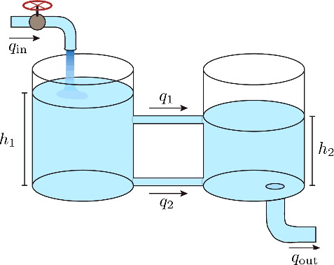
The control input is the inflow to tank 1: u = q _in. The levels in the tanks h ₁ and h ₂ form the states of the system and are governed by the flows q _1/2 between the tanks $$\begin{array}{cc}\hfill q_1& =C_{p1}\text{sgn}(h_1-h_2)\left(g\right|(1+\text{sgn}(h_1-h_c))(h_1-h_c)\hfill \\ & -(1+\text{sgn}(h_2-h_c))(h_2-h_c)|{)}^{\frac{1}{2}},\hfill \\ \hfill q_2& =C_{p2}\text{sgn}(h_1-h_2)\sqrt{2g\left|h_1-h_2\right|},\hfill \end{array}$$and the outflow from the second tank $q_{\text{out}}=C_{\text{out}}\sqrt{2g{h}_2}$. The dynamics of the states are $$\begin{array}{c}\hfill {\dot{h}}_1=\frac{1}{C_{t1}}(u-q_1-q_2),{\dot{h}}_2=\frac{1}{C_{t2}}(q_1+q_2-q_{\text{out}}).\end{array}$$Note that the system dynamics are on the one hand non-linear due to the Bernoulli equation and on the other hand hybrid due to the sudden change in dynamics as the level h ₁ rises above the connecting pipe. Hence, this example is the first showcase of the proposed parameter identifiers to simultaneously approximate non-linear and hybrid effects by PWA systems.

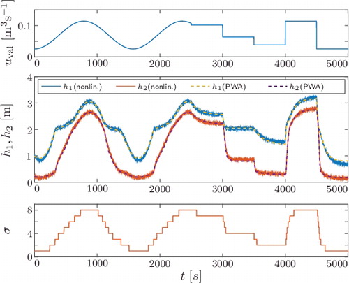
The maximal inflow u _max = 0.127 m³/s, at which the tanks will overflow, limits the controlled inflow u. The system is excited by two sinusoidal signals with amplitudes 0.3u _max and with frequencies 0.4 and 1 rad/s. Furthermore, a triangle-like offset that alternates between 0.2u _max and 0.9u _max is added to u and Gaussian noise $\mathcal{N}(0,0.003)$ is added to the measured tank levels.

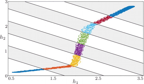
For the a-priori partitioning of the state-input space, we incorporate the previous knowledge that the system does not switch with respect to the inflow u. Hence, only the two-dimensional state-space is partitioned. The state-space partitions together with the state-space trajectory obtained with the excitation signal are shown in Figure 10. The figure at the same time suggests that the system may not be approximated well by an LTI model.

Figure 10. State-space trajectory for excitation with triangle-like offset and two sinusoidal signals. The state-space partitions are given by gray and white stripes.

The concurrent learning design parameters are A _m = −I _n , P = I _n , Γ = I _{n(n + p + 1)}, q = 18 and ν = 0.03. We excited the system for 4000 s and the parameter estimates in each subsystem converged about 500 s after the corresponding history stacks satisfied Assumption 3.1.

The comparison between the estimated PWA system and the hybrid two tank is shown in Figure 11. The excitation for this experiment differs from the training data which was used to estimate the model parameters. As can be seen from the figure, the estimated PWA system approximates well the non-linear, switching dynamics of the hybrid two-tank system.

Figure 11. Comparison of the hybrid two-tank system with the obtained PWA model for the validation input $u_{val}$.

6. Conclusions

This paper extends linear parameter identifiers to switched systems in the form of PWL and PWA systems. In the case of PWA systems, it is shown that the affine input violates classical assumptions on the richness of input signals. This violation is compensated by restricting the applicability to invertible system matrices. A neat state reset associated with detected switches secures stability of the estimation process, even for arbitrarily fast switching. Despite the maintained stability, fast switching does affect the rate of convergence. The proposed parameter identifiers for PWA systems are further improved by concurrent learning, where recorded data are used concurrently with instantaneous data. In the switched system setting, this allows to adapt even currently inactive parameter estimates and yields faster convergence. Furthermore, it is shown that the main drawback of concurrent learning, caused by outdated or erroneous history stack elements, can be overcome by the proposed outlier detection algorithm. Numerical simulations of both theoretical systems as well as a non-linear hybrid two-tank system validate the performance of parameter identifiers using concurrent learning. Future work focuses on deriving identifiers for systems with partial state measurement and unknown state-space partitions.

Disclosure statement

No potential conflict of interest was reported by the authors.

Additional information

Funding

The research leading to these results has received funding partly from the European Research Council under the European Union's Seventh Framework Programme (FP/2007–2013) ERC Grant Agreement [grant number 267877] and partly from the Technische Universität München – Institute for Advanced Study (www.tum-ias.de), funded by the German Excellence Initiative.

Appendix A. Definitions and lemmas

This appendix repeats definitions and lemmas from Ioannou and Sun (1996) which are needed for the convergence proofs in this paper. Another excellent introduction to the field of adaptive control is Narendra and Annaswamy (2005). PE plays a fundamental role in the convergence of adaptive systems.

Definition A.1

(Ioannou & Sun, 1996, Def. 4.3.1): A piecewise continuous signal vector $z:{\mathbb{R}}^{+}\to {\mathbb{R}}^n$ is persistently excited in ${\mathbb{R}}^n$ with a level of excitation α₀ > 0 if there exist constants α₁, T ₀ > 0 such that $$\begin{array}{c}\hfill {\alpha }_1{I}_n\ge \frac{1}{T_0}{\int }_t^{t+T_0}z\left(\tau \right)z^{\top }\left(\tau \right)d\tau \ge {\alpha }_0{I}_n,\forall t\ge 0.\end{array}$$

The following lemmas are used to prove convergence in Theorem 2.1 and Lemma 2.1 in Section 2.

Lemma A.1

(Ioannou & Sun, 1996, Lem. 5.6.1): If the auto-covariance of a function $z:{\mathbb{R}}^{+}\to {\mathbb{R}}^n$ defined as $$\begin{array}{c}\hfill R_z\left(t\right)\triangleq \underset{T\to \infty }{lim}\frac{1}{T}{\int }_{t_0}^{t_0+T}z\left(\tau \right)z^{\top }(t+\tau )d\tau \end{array}$$exists and is uniform with respect to t ₀, then z is persistently exciting if and only if R _z (0) is positive definite.

Lemma A.2

(Ioannou & Sun, 1996, Lem. 5.6.3): Consider the system described by (A1) $$\begin{array}{c}\hfill \left[\begin{array}{c}{\dot{\xi }}_1\\ {\dot{\xi }}_2\end{array}\right]=\left[\begin{array}{cc}\mathcal{A}& F^{\top }\left(t\right)\\ -P_{1}F\left(t\right)P_2& 0\end{array}\right]\left[\begin{array}{c}{\xi }_1\\ {\xi }_2\end{array}\right],\end{array}$$(A1) where ${\xi }_1\in {\mathbb{R}}^{n_1}$, ${\xi }_2\in {\mathbb{R}}^{g{n}_1}$ for some integer g, n ₁ ≥ 1, and $\mathcal{A},P_1,P_2$ are constant matrices and F(t) is of the form $$\begin{array}{c}\hfill F\left(t\right)=\left[\begin{array}{c}{z}_1\left(t\right)I_{n_1}\\ z_2\left(t\right)I_{n_1}\\ ⋮\\ z_r\left(t\right)I_{n_1}\end{array}\right]\in {\mathbb{R}}^{g{n}_1\times n_1},\end{array}$$where z _i , i = 1, 2,… , g are the elements of the vector $z\in {\mathbb{R}}^g$. Suppose that z is persistently excited and there exists a matrix P ₀ > 0 such that (A2) $$\begin{array}{c}\hfill {\dot{P}}_0+A_0^{\top }{P}_0+P_0{A}_0+C_0{C}_0^{\top }\le 0\end{array}$$(A2) where $$\begin{array}{c}\hfill A_0=\left[\begin{array}{cc}\mathcal{A}& F^{\top }\left(t\right)\\ -P_{1}F\left(t\right)P_2& 0\end{array}\right],C_0^{\top }=\left[I_{n_1},0\right].\end{array}$$Then, the equilibrium ξ_1e = 0, ξ_2e = 0 of Equation (A1(A1) $$\begin{array}{c}\hfill \left[\begin{array}{c}{\dot{\xi }}_1\\ {\dot{\xi }}_2\end{array}\right]=\left[\begin{array}{cc}\mathcal{A}& F^{\top }\left(t\right)\\ -P_{1}F\left(t\right)P_2& 0\end{array}\right]\left[\begin{array}{c}{\xi }_1\\ {\xi }_2\end{array}\right],\end{array}$$(A1) ) is exponentially stable in the large.

For PWA systems, the PE condition on z in Lemma A.2 can be guaranteed by Lemma 2.1, which is proposed in Section 2. The corresponding proof is given here for improved readability.

Proof of Lemma  2.1:

Lemma 2.1 is shown with the help of Lemma A.1 and a frequency domain relationship between z and the inputs u. Note that the affine term f can be seen as the input matrix of an additional constant input of 1. Therefore, let z be related to the constant input via a transfer function H _f (s). Furthermore, let the transfer function H _k (s) relate z to the kth input u _k . The dimensions of H _f (s) and H _k (s) are (n + p + 1) × 1. Overall, z is related to the inputs by $$\begin{array}{c}\hfill z\left(s\right)=\underset{H_f\left(s\right)}{\underbrace{\left[\begin{array}{c}{\left(s{I}_n-A\right)}^{-1}f\\ {\ell }_{p+1}\end{array}\right]}}1\left(s\right)+\sum _{k=1}^p\underset{H_k\left(s\right)}{\underbrace{\left[\begin{array}{c}{\left(s{I}_n-A\right)}^{-1}{b}_k\\ {\ell }_k\end{array}\right]}}{u}_k\left(s\right),\end{array}$$where b _k denotes the kth column of B and ${\ell }_k,{\ell }_{p+1}\in {\mathbb{R}}^{p+1}$ denote the kth and (p + 1)th column of the identity matrix $I_{p+1}\in {\mathbb{R}}^{(p+1)\times (p+1)}$, i.e.: $$\begin{array}{cc}\hfill {\ell }_k& ={[0\cdots 0\underset{k\text{th}\text{element}}{\underbrace{1}}0\cdots 00]}^{\top },\hfill \\ \hfill {\ell }_{p+1}& ={[0\cdots 000\cdots 01]}^{\top }.\hfill \end{array}$$

Under the assumption of distinct input frequencies, the auto covariance of z is given by (A3) $$\begin{array}{ccc}\hfill R_z\left(0\right)& =& \frac{1}{2\pi }{\int }_{-\infty }^{\infty }{H}_f(-j\omega )S_1\left(\omega \right)H_f^{\top }\left(j\omega \right)d\omega \hfill \\ & & +\frac{1}{2\pi }\sum _{k=1}^p{\int }_{-\infty }^{\infty }{H}_k(-j\omega )S_{u_k}\left(\omega \right)H_k^{\top }\left(j\omega \right)d\omega \hfill \end{array}$$(A3) where S ₁(ω) and $S_{u_k}\left(\omega \right)$ are the spectral distributions of the constant input 1 and the input u _k , respectively. Since u _k is sufficiently rich of order n + 1, its spectrum has n + 1 distinct peaks ${\mathcal{F}}_{u_k}\left({\omega }_{kl}\right)$ at frequencies ω _kl , l = 1, …n + 1. The affine term f results in a spectral peak at zero. The spectral distributions are (A4) $$\begin{array}{c}\hfill S_1\left(\omega \right)=\delta \left(\omega \right),S_{u_k}\left(\omega \right)=\sum _{l=1}^{n+1}{\mathcal{F}}_{u_k}\left({\omega }_{kl}\right)\delta (\omega -{\omega }_{kl}),\end{array}$$(A4) where δ(ω = 0) = 1 and δ(ω ≠ 0) = 0. With Equation (A4(A4) $$\begin{array}{c}\hfill S_1\left(\omega \right)=\delta \left(\omega \right),S_{u_k}\left(\omega \right)=\sum _{l=1}^{n+1}{\mathcal{F}}_{u_k}\left({\omega }_{kl}\right)\delta (\omega -{\omega }_{kl}),\end{array}$$(A4) ), the integrals in Equation (A3(A3) $$\begin{array}{ccc}\hfill R_z\left(0\right)& =& \frac{1}{2\pi }{\int }_{-\infty }^{\infty }{H}_f(-j\omega )S_1\left(\omega \right)H_f^{\top }\left(j\omega \right)d\omega \hfill \\ & & +\frac{1}{2\pi }\sum _{k=1}^p{\int }_{-\infty }^{\infty }{H}_k(-j\omega )S_{u_k}\left(\omega \right)H_k^{\top }\left(j\omega \right)d\omega \hfill \end{array}$$(A3) ) are replaced by summations: (A5) $$\begin{array}{ccc}\hfill R_z\left(0\right)& =& \frac{1}{2\pi }{H}_f(-j0)H_f^{\top }\left(j0\right)\hfill \\ & & +\frac{1}{2\pi }\sum _{k=1}^p\sum _{l=1}^{n+1}{\mathcal{F}}_{u_k}\left({\omega }_{kl}\right)H_k(-j{\omega }_{kl})H_k^{\top }\left(j{\omega }_{kl}\right).\hfill \end{array}$$(A5)

According to Lemma A.1, the vector z is persistently exciting if Equation (A5(A5) $$\begin{array}{ccc}\hfill R_z\left(0\right)& =& \frac{1}{2\pi }{H}_f(-j0)H_f^{\top }\left(j0\right)\hfill \\ & & +\frac{1}{2\pi }\sum _{k=1}^p\sum _{l=1}^{n+1}{\mathcal{F}}_{u_k}\left({\omega }_{kl}\right)H_k(-j{\omega }_{kl})H_k^{\top }\left(j{\omega }_{kl}\right).\hfill \end{array}$$(A5) ) is positive definite, i.e. the quadratic equation (A6) $$\begin{array}{c}\hfill {\chi }^{\top }{R}_z\left(0\right)\chi =0,\chi \in {\mathbb{R}}^{n+p+1}\end{array}$$(A6) can only have a single solution at χ = 0 _{n + p + 1}. Note that the outer products H _k ( − jω _kl )H _k (jω _kl )^⊤ of the column vectors H _k (jω _kl ) are positive semi-definite. Therefore, each summand in Equation (A5(A5) $$\begin{array}{ccc}\hfill R_z\left(0\right)& =& \frac{1}{2\pi }{H}_f(-j0)H_f^{\top }\left(j0\right)\hfill \\ & & +\frac{1}{2\pi }\sum _{k=1}^p\sum _{l=1}^{n+1}{\mathcal{F}}_{u_k}\left({\omega }_{kl}\right)H_k(-j{\omega }_{kl})H_k^{\top }\left(j{\omega }_{kl}\right).\hfill \end{array}$$(A5) ) is positive semi-definite and Equation (A6(A6) $$\begin{array}{c}\hfill {\chi }^{\top }{R}_z\left(0\right)\chi =0,\chi \in {\mathbb{R}}^{n+p+1}\end{array}$$(A6) ) is equivalent to (A7) $${\chi }^{\top }{R}_z\left(0\right)\chi =\underset{\ge 0}{\underbrace{{\chi }^{\top }{R}_{z1}\left(0\right)\chi }}+\underset{\ge 0}{\underbrace{{\chi }^{\top }{R}_{z2}\left(0\right)\chi }}=0,$$(A7) where $$\begin{array}{cc}\hfill R_{z1}\left(0\right)& \triangleq \frac{1}{2\pi }\sum _{k=1}^p\sum _{l=1}^{n+1}{\mathcal{F}}_{u_k}\left({\omega }_{kl}\right)H_k(-j{\omega }_{kl})H_k^{\top }\left(j{\omega }_{kl}\right),\hfill \\ \hfill R_{z2}\left(0\right)& \triangleq \frac{1}{2\pi }{H}_f(-j0)H_f^{\top }\left(j0\right).\hfill \end{array}$$

First, χ^⊤ R _z1(0)χ = 0 is solved for χ. As all the summands of R _z1(0) are positive semi-definite, this equality only holds if $${\chi }^{\top }{H}_k(-j{\omega }_{kl})H_k^{\top }\left(j{\omega }_{kl}\right)\chi =0\begin{array}{cc}& k=1,2,\dots ,p,\hfill \\ & l=1,2,\dots ,n+1,\hfill \end{array}$$or equivalently (A8) $$\begin{array}{c}\hfill H_k^{\top }\left(j{\omega }_{kl}\right)\chi =0\begin{array}{cc}& k=1,2,\dots ,p,\hfill \\ & l=1,2,\dots ,n+1.\hfill \end{array}\end{array}$$(A8) The transfer function H _k (s) can also be written as (A9) $$H_k\left(s\right)=\frac{1}{a\left(s\right)}\left[\begin{array}{c}\text{adj}(s{I}_n-A)b_k\\ a\left(s\right){\ell }_k\end{array}\right]=\frac{1}{a\left(s\right)}{\bar{H}}_k\left(s\right),$$(A9) where $a\left(s\right)=det(s{I}_n-A)$. Therefore, the equalities (A8(A8) $$\begin{array}{c}\hfill H_k^{\top }\left(j{\omega }_{kl}\right)\chi =0\begin{array}{cc}& k=1,2,\dots ,p,\hfill \\ & l=1,2,\dots ,n+1.\hfill \end{array}\end{array}$$(A8) ) are also equivalent to (A10) $$\begin{array}{c}\hfill {\bar{H}}_k^{\top }\left(j{\omega }_{kl}\right)\chi =0\begin{array}{cc}& k=1,2,\dots ,p,\hfill \\ & l=1,2,\dots ,n+1.\hfill \end{array}\end{array}$$(A10)

Each vector element of ${\bar{H}}_k\left(j{\omega }_{kl}\right)$ is a polynomial in ω _kl of maximal order n (see Equation (A9(A9) $$H_k\left(s\right)=\frac{1}{a\left(s\right)}\left[\begin{array}{c}\text{adj}(s{I}_n-A)b_k\\ a\left(s\right){\ell }_k\end{array}\right]=\frac{1}{a\left(s\right)}{\bar{H}}_k\left(s\right),$$(A9) )). So after multiplying with χ, $g_k\left(s\right)\triangleq {\bar{H}}_k^{\top }\left(s\right)\chi$ is also a polynomial in s of maximal order n. For a given k, Equation (A10(A10) $$\begin{array}{c}\hfill {\bar{H}}_k^{\top }\left(j{\omega }_{kl}\right)\chi =0\begin{array}{cc}& k=1,2,\dots ,p,\hfill \\ & l=1,2,\dots ,n+1.\hfill \end{array}\end{array}$$(A10) ) states that g _k (s) is zero at n + 1 frequencies or values of s. As g _k (s) is only of order n, it follows that $g_k\left(s\right)=0,\forall s\in \mathbb{C},k=1,\dots ,p$. Combining the p equalities of Equation (A10(A10) $$\begin{array}{c}\hfill {\bar{H}}_k^{\top }\left(j{\omega }_{kl}\right)\chi =0\begin{array}{cc}& k=1,2,\dots ,p,\hfill \\ & l=1,2,\dots ,n+1.\hfill \end{array}\end{array}$$(A10) ) in matrix form gives (A11) $$\begin{array}{c}\hfill {\left[\begin{array}{c}\text{adj}(s{I}_n-A)B\\ a\left(s\right)I_p\\ 0_p^{\top }\end{array}\right]}^{\top }\chi =0_p,\end{array}$$(A11) where $0_p\in {\mathbb{R}}^p$ is a p-dimensional zero vector. Next, the vector χ is expressed as $\chi ={[{\mathcal{X}}^{\top },{\mathcal{Y}}^{\top },\mathcal{Z}]}^{\top }$, with $\mathcal{X}={[{\chi }_1,\dots ,{\chi }_n]}^{\top }\in {\mathbb{R}}^n$, $\mathcal{Y}={[{\chi }_{n+1},\dots ,{\chi }_{n+p}]}^{\top }\in {\mathbb{R}}^p$ and $\mathcal{Z}={\chi }_{n+p+1}\in \mathbb{R}$. This leads to (A12) $$\begin{array}{c}\hfill {\left(\text{adj}(s{I}_n-A)B\right)}^{\top }\mathcal{X}+a\left(s\right)\mathcal{Y}+0_p\mathcal{Z}=0_p.\end{array}$$(A12)

The following expressions for adj(sI _n − A)B and a(s) are applied to Equation (A12(A12) $$\begin{array}{c}\hfill {\left(\text{adj}(s{I}_n-A)B\right)}^{\top }\mathcal{X}+a\left(s\right)\mathcal{Y}+0_p\mathcal{Z}=0_p.\end{array}$$(A12) ) $$\begin{array}{cc}\hfill \text{adj}(sI-A)B=& B{s}^{n-1}+(AB+a_{n-1}B)s^{n-2}\hfill \\ & +(A^{2}B+a_{n-1}AB+a_{n-2}B)s^{n-3}\hfill \\ & +\cdots +(A^{n-1}B+a_{n-1}{A}^{n-2}B+\cdots +a_{1}B),\hfill \\ \hfill a\left(s\right)=& s^n+a_{n-1}{s}^{n-1}+\cdots +a_{1}s+a_0,\hfill \end{array}$$which results in a polynomial of order n. All coefficients of the resulting polynomial must be zero, so that the polynomial is zero independent of s. This leads to n equalities that can be written in a compact form: $$\begin{array}{c}\hfill \mathcal{Y}=0_p\text{and}{[B,AB,\dots ,A^{n-1}B]}^{\top }\mathcal{X}=0_{np}.\end{array}$$

With (A, B) controllable, it follows that the matrix [B, AB,… , A ^{n − 1} B] is of full rank. Therefore, the equality (A12(A12) $$\begin{array}{c}\hfill {\left(\text{adj}(s{I}_n-A)B\right)}^{\top }\mathcal{X}+a\left(s\right)\mathcal{Y}+0_p\mathcal{Z}=0_p.\end{array}$$(A12) ) holds for $\mathcal{X}=0_n$, $\mathcal{Y}=0_p$ and an arbitrary $\mathcal{Z}\in \mathbb{R}$. Consequently, R _z1(0) is only positive semi-definite. Therefore, R _z2(0) in Equation (A7(A7) $${\chi }^{\top }{R}_z\left(0\right)\chi =\underset{\ge 0}{\underbrace{{\chi }^{\top }{R}_{z1}\left(0\right)\chi }}+\underset{\ge 0}{\underbrace{{\chi }^{\top }{R}_{z2}\left(0\right)\chi }}=0,$$(A7) ) must restrict the choice of $\mathcal{Z}$ further, i.e. χ^⊤ R _z2(0)χ = 0 for $\mathcal{X}=0_n$, $\mathcal{Y}=0_p$ and $\mathcal{Z}=0$. The same arguments as above lead to $$\begin{array}{c}\hfill {\bar{H}}_f^{\top }\left(j0\right)\chi ={\left[\begin{array}{c}\text{adj}(-A)f\\ 0_p\\ a\left(j0\right)\end{array}\right]}^{\top }\chi =0,\end{array}$$and with $\chi ={[{\mathcal{X}}^{\top },{\mathcal{Y}}^{\top },\mathcal{Z}]}^{\top }$ result in (A13) $$\begin{array}{c}\hfill {\left(\text{adj}(-A)f\right)}^{\top }\mathcal{X}+a\left(j0\right)\mathcal{Z}=0.\end{array}$$(A13)

Since R _z1(0) and R _z2(0) are both positive semi-definite, one needs to find those χ for which χ^⊤ R _z1(0)χ = 0 and χ^⊤ R _z2(0)χ = 0. In order to ensure χ^⊤ R _z1(0)χ = 0, it is thus necessary to assume $\mathcal{X}=0_n$ and $\mathcal{Y}=0_p$ in Equation (A13(A13) $$\begin{array}{c}\hfill {\left(\text{adj}(-A)f\right)}^{\top }\mathcal{X}+a\left(j0\right)\mathcal{Z}=0.\end{array}$$(A13) ). With a(j0) = a ₀, Equation (A13(A13) $$\begin{array}{c}\hfill {\left(\text{adj}(-A)f\right)}^{\top }\mathcal{X}+a\left(j0\right)\mathcal{Z}=0.\end{array}$$(A13) ) reduces to a ₀ Z = 0. Since A is assumed to be invertible, we have a ₀ ≠ 0. Therefore, $\mathcal{Z}\stackrel{!}{=}0$ in order to ensure ${\bar{H}}_f^{\top }\left(j0\right)\chi =0$ with $\mathcal{X}=0_n$ and $\mathcal{Y}=0_p$. This shows that χ^⊤ R _z (0)χ = 0 only holds for χ = 0 _{n + p + 1} and thus proves positive definiteness of R _z (0) and according to Lemma A.1 makes z persistently exciting.

References

- Azuma, S. , Imura, J. , & Sugie, T. (2010). Lebesgue piecewise affine approximation of nonlinear systems. Nonlinear Analysis: Hybrid Systems, 4 (1), 92–102.
- Bako, L. (2014). Subspace clustering through parametric representation and sparse optimization. IEEE Signal Processing Letters, 21 (3), 356–360.
- Bako, L. , Boukharouba, K. , Duviella, E. , & Lecoeuche, S. (2011). A recursive identification algorithm for switched linear/affine models. Nonlinear Analysis: Hybrid Systems, 5 (2), 242–253.
- Bako, L. , Mercère, G. , & Lecoeuche, S. (2009). On-line structured subspace identification with application to switched linear systems. International Journal of Control, 82 (8), 1496–1515.
- Bako, L. , Mercère, G. , Vidal, R. , & Lecoeuche, S . (2009, July). Identification of switched linear state space models without minimum dwell time. In E. Walter (Eds.), Proceedings of the 15th IFAC symposium on system identification (pp. 569–574). Saint-Malo, France: Elsevier.
- Bako, L. , van Luong, L. , Lauer, F. , & Bloch, G . (2013, June). Identification of MIMO switched state-space models. In Proceedings of the american control conference (ACC) (pp. 71–76). Washington, DC: IEEE.
- Bamieh, B. , & Giarré, L. (2002). Identification of linear parameter varying models. International Journal of Robust and Nonlinear Control, 12 (9), 841–853.
- Blackmore, L. , Gil, S. , Seung, C. , & Williams, B . (2007, December). Model learning for switching linear systems with autonomous mode transitions. In 46th IEEE conference on decision and control (pp. 4648–4655). New Orleans, LA: IEEE.
- Branicky, M. S. (1998). Multiple Lyapunov functions and other analysis tools for switched and hybrid systems. IEEE Transactions on Automatic Control, 43 (4), 475–482.
- Chen, D. , Bako, L. , & Lecoeuche, S . (2011, September). A recursive sparse learning method: Application to jump Markov linear systems. In S. Bittanti (Eds.), Proceedings of the 18th IFAC world congress (pp. 3198–3203). Milan, Italy: Elsevier.
- Chowdhary, G. (2010). Concurrent learning for convergence in adaptive control without persistency of excitation ( Unpublished doctoral dissertation). Atlanta, GA: Georgia Institute of Technology.
- Chowdhary, G. , & Johnson, E . (2010, December). Concurrent learning for convergence in adaptive control without persistency of excitation. In Proceedings of the 49th IEEE conference on decision and control (CDC) (pp. 3674–3679). Atlanta, GA: IEEE.
- Chowdhary, G. , Mühlegg, M. , How, J. P , & Holzapfel, F . (2013, December). A concurrent learning adaptive-optimal control architecture for nonlinear systems. In Proceedings of the 52nd IEEE conference on decision and control (pp. 868–873). Firenze, Italy: IEEE.
- Chowdhary, G. , Mühlegg, M. , & Johnson, E. (2014). Exponential parameter and tracking error convergence guarantees for adaptive controllers without persistency of excitation. International Journal of Control, 87 (8), 1583–1603.
- Chowdhary, G. , Yucelen, T. , Mühlegg, M. , & Johnson, E. N. (2013). Concurrent learning adaptive control of linear systems with exponentially convergent bounds. International Journal of Adaptive Control and Signal Processing, 27 , 280–301.
- De La Torre, G. , Chowdhary, G. , & Johnson, E. N . (2013, June). Concurrent learning adaptive control for linear switched systems. In Proceedings of the American control conference (ACC) (pp. 854–859). Washington, DC: IEEE.
- Di Bernardo, M. , Montanaro, U. , & Santini, S . (2008, December). Novel switched model reference adaptive control for continuous piecewise affine systems. In Proceedings of the 47th IEEE conference on decision and control (pp. 1925–1930). Cancun, Mexico: IEEE.
- Di Bernardo, M. , Montanaro, U. , & Santini, S . (2009, December). Hybrid minimal control synthesis identification of continuous piecewise linear systems. In Proceedings of the 48th IEEE conference on decision and control and 28th chinese control conference (pp. 3188–3193). Shanghai, China: IEEE.
- Di Bernardo, M. , Montanaro, U. , & Santini, S. (2013). Hybrid model reference adaptive control of piecewise affine systems. IEEE Transactions on Automatic Control, 58 (2), 304–316.
- Feiler, M. J. , & Narendra, K . (2006, December). Simultaneous identification and control of time-varying systems. In Proceedings of the 45th IEEE conference on decision and control (pp. 1093–1098). San Diego, CA: IEEE.
- Feiler, M. J. , & Narendra, K . (2008, June). Identification and control using multiple models. In Proceedings of the 14th Yale workshop on adaptive and learning systems (pp. 33–42). New Haven, CT: Yale University Center of Systems Science.
- Ferrari-Trecate, G. , Muselli, M. , Liberati, D. , & Morari, M. (2003). A clustering technique for the identification of piecewise affine systems. Automatica, 39 (2), 205–217.
- Garnier, H. (2015). Direct continuous-time approaches to system identification. Overview and benefits for practical applications. European Journal of Control, 24 , 50–62.
- Garulli, A. , Paoletti, S. , & Vicino, A . (2012, July). A survey on switched and piecewise affine system identification. In Proceedings of the 16th IFAC Symposium on system identification (pp. 344–355). Brussels, Belgium: Elsevier.
- Gil, S. , & Williams, B . (2009, December). Beyond local optimality: An improved approach to hybrid model learning. In Proceedings of the 48th IEEE conference on decision and control and 28th Chinese control conference (pp. 3938–3945). Shanghai, China: IEEE.
- Heemels, W. P. M. H. , Schutter, B. D. , & Bemporad, A. (2001). Equivalence of hybrid dynamical models. Automatica, 37 (7), 1085–1091.
- Ioannou, P. , & Sun, J . (1996). Robust adaptive control . Upper Saddle River, NJ: Prentice-Hall.
- Jazwinski, A. H . (1970). Stochastic processes and filtering theory . New York, NY: Academic Press.
- Kamalapurkar, R. , Walters, P. , & Dixon, W. E. (2016). Model-based reinforcement learning for approximate optimal regulation. Automatica, 64 , 94–104.
- Kersting, S. , & Buss, M . (2014a, June). Adaptive identification of continuous-time switched linear and piecewise linear systems. In Proceedings of the European control conference (ECC) (pp. 31–36). Strasbourg, France: IEEE.
- Kersting, S. , & Buss, M . (2014b, December). Concurrent learning adaptive identification of piecewise affine systems. In Proceedings of the 53rd IEEE conference on decision and control (CDC) (pp. 3930–3935). Los Angeles, CA: IEEE.
- Kersting, S. , & Buss, M. (2014c, July). Online identification of piecewise affine systems. In Proceedings of the UKACC 10th international conference on control (pp. 90–95). Loughborough, UK: IEEE.
- Kersting, S. , & Buss, M . (2015, December). Removing erroneous history stack elements in concurrent learning. In Proceedings of the IEEE 54th annual conference on decision and control (pp. 7604–7609). Osaka, Japan: IEEE.
- Klotz, J. , Kamalapurkar, R. , & Dixon, W. E . (2014, June). Concurrent learning-based network synchronization. In Proceedings of the American control conference (ACC) (pp. 796–801). Portland, OR: IEEE.
- Lauer, F. , Bloch, G. , & Vidal, R. (2011). A continuous optimization framework for hybrid system identification. Automatica, 47 (3), 608–613.
- Liberzon, D . (2003). Switching in systems and control . New York, NY: Springer Science+Business Media.
- Ljung, L. (1987). System identification: Theory for the user . Englewood Cliffs, NJ: Prentice-Hall.
- Lopes, L. R. , Borges, G. A. , & Ishihara, J. Y . (2013, June). New algorithm for identification of discrete-time switched linear systems. In Proceedings of the American control conference (ACC) (pp. 6219–6224). Washington, DC: IEEE.
- Maruta, I. , Sugie, T. , & Kim, T . (2011, September). Identification of multiple mode models via distributed particle swarm optimization. In S. Bittanti (Eds.) Proceedings of the 18th IFAC world congress (pp. 7743–7748). Milan, Italy: Elsevier.
- Modares, H. , Lewis, F. L. , & Naghibi-Sistani, M.-B. (2014). Integral reinforcement learning and experience replay for adaptive optimal control of partially-unknown constrained-input continuous-time systems. Automatica, 50 (1), 193–202.
- Narendra, K. , & Annaswamy, A. M . (2005). Stable adaptive systems . Mineola, NY: Dover Publications.
- Paoletti, S. , Juloski, A. L. , Ferrari-Trecate, G. , & Vidal, R . (2007). Identification of hybrid systems: A tutorial. European Journal of Control, 13 (2–3), 242–260.
- Pekpe, K. M. , & Lecœuche, S . (2008). Online clustering of switching models based on a subspace framework. Nonlinear Analysis: Hybrid Systems, 2 (3), 735–749.
- Petreczky, M. (2011). Realization theory for linear and bilinear switched systems: A formal power series approach. ESAIM: Control, Optimisation and Calculus of Variations, 17 (2), 410–445.
- Petreczky, M. , & Bako, L . (2011, December). On the notion of persistence of excitation for linear switched systems. In Proceedings of the 50th IEEE conference on decision and control and european control conference (CDC-ECC) (pp. 1840–1847). Orlando, FL: IEEE.
- Petreczky, M. , Bako, L. , & van Schuppen, J. H . (2010, April). Identifiability of discrete-time linear switched systems. In Proceedings of the 13th ACM international conference on hybrid systems: Computation and control (pp. 141–150). Stockholm, Sweden: ACM.
- Petreczky, M. , & van Schuppen, J. H. (2010). Realization theory for linear hybrid systems. IEEE Transactions on Automatic Control, 55 (10), 2282–2297.
- Petreczky, M. , & van Schuppen, J. H. (2011). Partial-realization theory for linear switched systems – a formal power series approach. Automatica, 47 (10), 2177–2184.
- Sang, Q. , & Tao, G . (2012). Adaptive control of piecewise linear systems: The state tracking case. IEEE Transactions on Automatic Control, 57 (2), 522–528.
- Shumway, R. H. , & Stoffer, D. S . (2006). Time series analysis and its applications: With R examples (2nd updated ed.). New York, NY: Springer.
- Simon, D . (2006). Optimal state estimation: Kalman, H [infinity] and nonlinear approaches . Hoboken, NJ: Wiley-Interscience.
- Tóth, R. (2010). Modeling and identification of linear parameter-varying systems (Vol. 403). Berlin: Springer.
- Verdult, V. , & Verhaegen, M. (2002). Subspace identification of multivariable linear parameter-varying systems. Automatica, 38 (5), 805–814.
- Vidal, R . (2008). Recursive identification of switched ARX systems. Automatica, 44 (9), 2274–2287.
- Vidal, R. , Soatto, S. , Yi, M. , & Sastry, S. (2003, December). An algebraic geometric approach to the identification of a class of linear hybrid systems. In Proceedings of the 42nd IEEE conference on decision and control (pp. 167–172). Maui, HI: IEEE.
- Wang, J. , & Chen, T. (2011, March). Online identification of switched linear output error models. In Proceedings of the IEEE international symposium on computer-aided control system design (CACSD) (pp. 1379–1384). Tucson, AZ: IEEE.
- Wawrzyński, P . (2009). Real-time reinforcement learning by sequential actor–critics and experience replay. Neural Networks, 22 (10), 1484–1497.