Infinite horizon cancer treatment model with isoperimetrical constraint: existence of optimal solutions and numerical analysis

ABSTRACT

In this paper, a class of infinite horizon optimal control problems with a mixed control-state isoperimetrical constraint, also interpreted as a budget constraint, is considered. The underlying dynamics is assumed to be affine-linear in control. The crucial idea which is followed in this paper is the choice of a weighted Sobolev space as the state space. For this class of problems, we establish an existence result and apply it to a bilinear model of optimal cancer treatment with an isoperimetrical constraint including the overall amount of drugs used during the whole therapy horizon. A numerical analysis of this model is provided by means of open source software package OCMat, which implements a continuation method for solving discounted infinite horizon optimal control problems.

KEYWORDS:

• Infinite horizon optimal control
• existence theorem
• weighted Sobolev spaces
• model of cancer treatment
• numerical solution

View correction statement:

Erratum

1. Introduction

Infinite horizon optimal control problems have been investigated since the 1970s of the last century, cf. Aseev and Kryazhimskii (2007), Aseev and Veliov (2012, 2014), Carlson, Haurie, and Leizarowitz (1991), Garg, Hager, and Rao (2011), Halkin (1979), Zaslavski (2006, 2014) and among many others. This class of problems finds many applications in the economics, biology and stabilisation problems as well, cf. Feichtinger and Hartl (1986) and Grass, Caulkins, Feichtinger, Tragler, and Behrens (2008). The interest of introducing an isoperimetrical constraint in an optimal control problem, also often called budget constraint, is motivated by many reasons, e.g. from the point of view of multicriterial control problems (see Torres 2006, p. 176), or by evident economical arguments such as exhaustible resources or bounded budget (cf. Aseev, Besov, & Kaniovski, 2013; Feichtinger & Hartl, 1986, p. 122), or by therapeutic evidences (cf. Maurer & Pinho, 2015, p. 3; Ledzewicz, Maurer, & Schaettler, 2011, p. 307). Throughout the paper, the budget constraint is assumed to be linear in both the state and the control variables, while the underlying dynamics is assumed to be linear in control.

The main theoretical task of the present paper is to derive an existence result for the considered class of mixed budget-constrained optimal control problems with infinite horizon. On the other hand, the obtained existence theorem is to apply to an infinite horizon optimal control problem of cancer treatment which is of great practical interest. The main practical reason for investigating a cancer treatment model with infinite horizon consists in establishing structural changes in optimal solutions while passing from the model with a finite to a model with an infinite horizon. At the present time, mathematical models with a fix finite time horizon are used for computation of optimal cancer treatment strategies, cf. Schättler and Ledzewicz (2015). Their aim is mostly to eliminate all the tumour cells as fast as possible whereas the side-effects and the therapy costs should be minimised, the minimisation of the so-called damage functional should be guaranteed. The drawback of this method lies possibly in the choice of a very short time horizon which causes very high side-effects onto the entire human body, which are too high to be acceptable. These are the immune weakness, unnecessarily killed or damaged healthy tissues as well as the increased resistance of tumour cells. On the contrary, in the present paper we intend to investigate whether an infinite horizon model can provide less aggressive stabilising long-term therapies. These therapies might not necessarily lead to a tumour-free equilibrium of the dynamical system (human body), but to a ‘coexisting’ type of equilibrium, i.e. where tumour and normal cells coexist.

The numerical analysis of the formulated model will be performed with the help of the open source software package OCMat, cf. Graß (2012), which can be downloaded at http://orcos.tuwien.ac.at/research/ocmat_software/. This package implements an indirect numerical method for solving nonlinear discounted infinite horizon optimal control problems combining a continuation method with two-point boundary value problem solver. In contrast to direct methods, the used software attempts to avoid ‘cutting the horizon procedure’ while it uses a continuation method starting at a stationary solution, which is known to be optimal at the equilibrium point taken as an initial state point, and moving towards the given state initial condition, i.e. the continuation happens with respect to the initial condition. Among other existing indirect methods for solving infinite horizon problems we want to mention methods developed in Kunkel and Von Dem Hagen (2000) and Pickenhain, Burtchen, Kolo, and Lykina (2016). The first source provides a method based on a transformation technique which aims to transform the infinite horizon problem into an equivalent finite horizon problem by means of time transformation applied to the objective and to the dynamics and afterwards to solve two-point boundary value problems. However, the algorithm does not allow any constraints, i.e. state or control constraints. In the second source, the method is presently developed only for a class of linear-quadratic control problems which does not cover problems with bilinear dynamics such as cancer treatment optimal control problem presented and analysed in this paper. In case of extension of the pseudospectral method developed in Pickenhain et al. (2016), a comparison of the performance of both numerical methods would be of interest.

We also would like to emphasise the importance of obtaining existence theorems, which is especially true for problems, where the finding of analytical solutions is hardly possible. While applying numerical solution methods, it is necessary to know that the considered optimal control problem possesses an optimal solution indeed, otherwise applying the necessary optimality conditions in the form of Pontryagin Maximum Principle to find the solution becomes ‘naive’ heuristics. Available existence results help to justify the viability of obtained numerical results. One of the main assumptions of the numerical method applied here to analyse the infinite horizon cancer treatment problem is the existence of an optimal solution for all the initial states which belong to a certain compact subset of ${\mathrm{I}\mathrm{R}}^n$ (cf. Graß, 2012, p. 1628). This will be done analytically before applying the method.

The proof of the existence theorem presented in this paper follows the scheme of the generalised Weierstraß theorem. The crucial role in our investigations is played by the choice of a weighted Sobolev space as the state space and by the rigorous functional analytical approach in the proof of the Maximum Principle. Control problems with isoperimetric constraints were handled in many sources, e.g. Aseev et al. (2013), Feichtinger and Hartl (1986) and Torres (2006), but either not in the context of weighted Sobolev spaces or not on an unbounded interval of integration. The existence theorem obtained in Lykina and Pickenhain (2016) was generalised here due to the more general state equation.

The paper has the following structure. The second section contains important definitions. Section 3 introduces the problem statement and the optimality criterion. The derivation of the existence result is contained in Sections 4 and 5; we analyse the infinite horizon model of optimal cancer treatment with a budget constraint in order to demonstrate the applicability of the theoretical result proved before as well as to enlighten the structural changes compared to the corresponding finite horizon problem. A summary of the results concludes the paper.

2. Weighted Lebesgue and Sobolev spaces

Let us write $[0,\infty )={\mathrm{I}\mathrm{R}}_{+}$. We denote by $\phantom{(}\mathit{M}\left({\mathrm{I}\mathrm{R}}_{+}\right)$, ${\mathit{\text{Ł}}}_p\left({\mathrm{I}\mathrm{R}}_{+}\right)$ and ${\phantom{(}\mathit{C}}^0\left({\mathrm{I}\mathrm{R}}_{+}\right)$ the spaces of all functions $x:{\mathrm{I}\mathrm{R}}_{+}\to \mathrm{I}\mathrm{R}$ which are Lebesgue measurable, in the pth power Lebesgue integrable or continuous, respectively (see Dunford & Schwartz, 1988, pp. 146,  285; Elstrodt, 1996, p. 228). The Sobolev space ${\mathit{W}}_p^1\left({\mathrm{I}\mathrm{R}}_{+}\right)$ is then defined as the space of all functions $x:{\mathrm{I}\mathrm{R}}_{+}\to \mathrm{I}\mathrm{R}$ which belong to ${\mathit{\text{Ł}}}_p\left({\mathrm{I}\mathrm{R}}_{+}\right)$ and admit distributional derivative $\dot{x}$ (Yosida, 1974, p. 49) belonging to ${\mathit{L}}_p\left({\mathrm{I}\mathrm{R}}_{+}\right)$ as well.

Definition 2.1:

(a)	A continuous function $\nu :{\mathrm{I}\mathrm{R}}_{+}\to \mathrm{I}\mathrm{R}$ with positive values is called a weight function.
(b)	A weight function ν will be called a density function iff it is Lebesgue integrable over ${\mathrm{I}\mathrm{R}}_{+}$, i.e. ∫∞ 0ν(t) dt < ∞ (cf. Kufner, 1985, p. 18).
(c)	By means of a weight function $\nu \in {\phantom{(}\mathit{C}}^0\left({\mathrm{I}\mathrm{R}}_{+}\right)$ we define for any 1 ≤ p < ∞ the weighted Lebesgue space $$\begin{array}{ccc}\hfill {\mathit{\text{Ł}}}_p({\mathrm{I}\mathrm{R}}_{+},\nu )& =& \{x\in \phantom{(}\mathit{M}\left({\mathrm{I}\mathrm{R}}_{+}\right),|{\parallel x\parallel }_{{\mathit{\text{Ł}}}_p({\mathrm{I}\mathrm{R}}_{+},,\nu )}\hfill \\ & =& (\underset{0}{\overset{\infty }{\int }}{\left|x\left(t\right)\right|}^p\nu \left(t\right)dt{)}^{1/p}<\infty \}.\hfill \end{array}$$
(d)	For $x\in {\mathit{\text{Ł}}}_p({\mathrm{I}\mathrm{R}}_{+},,\nu )$ let the distributional derivative $\dot{x}$ be defined according to Yosida (1974, p. 46). We introduce the weighted Sobolev space of all ${\mathit{\text{Ł}}}_p({\mathrm{I}\mathrm{R}}_{+},,\nu )$ functions having its distributional derivative in ${\mathit{\text{Ł}}}_p({\mathrm{I}\mathrm{R}}_{+},,\nu )$: $$\begin{array}{c}\hfill {\mathit{W}}_p^1({\mathrm{I}\mathrm{R}}_{+},\nu )=\left\{x\in \phantom{(}\mathit{M}\left({\mathrm{I}\mathrm{R}}_{+}\right)|x\in {\mathit{\text{Ł}}}_p({\mathrm{I}\mathrm{R}}_{+},\nu ),\dot{x}\in {\mathit{\text{Ł}}}_p({\mathrm{I}\mathrm{R}}_{+},\nu )\right\}\end{array}$$(see Kufner, 1985, p. 11).

Equipped with the norm $$\begin{array}{c}\hfill {\parallel x\parallel }_{{\mathit{W}}_p^1({\mathrm{I}\mathrm{R}}_{+},,\nu )}={\parallel x\parallel }_{{\mathit{\text{Ł}}}_p({\mathrm{I}\mathrm{R}}_{+},,\nu )}+{\parallel \dot{x}\parallel }_{{\mathit{\text{Ł}}}_p({\mathrm{I}\mathrm{R}}_{+},,\nu )},\end{array}$$ ${\mathit{W}}_p^1({\mathrm{I}\mathrm{R}}_{+},\nu )$ becomes a Banach space (this can be confirmed analogously to Kufner, 1985, p. 19).

Lemma 2.1:

Let ν be a density function. Any linear continuous functional ϕ : ${\mathit{\text{L}}}_p({\mathrm{I}\mathrm{R}}_{+},\nu )\to \mathrm{I}\mathrm{R}$ can be represented by a function $\varphi \in {\mathit{L}}_q({\mathrm{I}\mathrm{R}}_{+},\nu )$ with p ⁻¹ + q ⁻¹ = 1 if 1 < p < ∞ and q = ∞ if p = 1: (1) $$\begin{array}{c}\hfill ⟨\varphi ,x⟩=\underset{0}{\overset{\infty }{\int }}\varphi \left(t\right)x\left(t\right)\nu \left(t\right)dt\forall x\in {\mathit{\text{L}}}_p({\mathrm{I}\mathrm{R}}_{+},\nu ).\end{array}$$(1)

Proof:

We may apply Elstrodt (1996, p. 287), since the measure generated by the density function ν is finite on ${\mathrm{I}\mathrm{R}}_{+}$.

For p = 2 the spaces ${\mathit{L}}_2({\mathrm{I}\mathrm{R}}_{+},,\nu )$ and ${\mathit{W}}_2^1({\mathrm{I}\mathrm{R}}_{+},\nu )$ become separable Hilbert spaces, see Kufner (1985), and (1(1) $$\begin{array}{c}\hfill ⟨\varphi ,x⟩=\underset{0}{\overset{\infty }{\int }}\varphi \left(t\right)x\left(t\right)\nu \left(t\right)dt\forall x\in {\mathit{\text{L}}}_p({\mathrm{I}\mathrm{R}}_{+},\nu ).\end{array}$$(1) ) is the scalar product in ${\mathit{L}}_2({\mathrm{I}\mathrm{R}}_{+},,\nu )$.

3. Problem formulation

The main control problem being considered in the present paper is (2) $$\begin{array}{c}\hfill {\left(\mathrm{P}\right)}_{\infty }^B:J_{\infty }(x,u)=\underset{0}{\overset{\infty }{\int }}r(t,x\left(t\right),u\left(t\right)){\nu }_0\left(t\right)dt⟶min\text{!}\end{array}$$(2) (3) $$\begin{array}{ccc}\hfill (x,u)& \in & {\mathit{W}}_2^{1,n}({\mathrm{I}\mathrm{R}}_{+},{\nu }_1)\times {\mathit{\text{L}}}_2^m({\mathrm{I}\mathrm{R}}_{+},{\nu }_1),,\hfill \end{array}$$(3) (4) $$\begin{array}{c}\hfill \dot{x}\left(t\right)=A(t,x\left(t\right))+B(t,x\left(t\right))u\left(t\right)\text{a.}\text{e.}\text{on}{\mathrm{I}\mathrm{R}}_{+},x\left(0\right)=x_0>0,\end{array}$$(4) (5) $$\begin{array}{ccc}\hfill d& ⩾& \underset{0}{\overset{\infty }{\int }}\left\{D_1^0{\left(t\right)}^{T}x\left(t\right)+D_2^0{\left(t\right)}^{T}u\left(t\right)\right\}{\nu }_2\left(t\right)dt\hfill \end{array}$$(5) (6) $$\begin{array}{ccc}\hfill u\left(t\right)& \in & U\text{a.}\text{e.}\text{on}{\mathrm{I}\mathrm{R}}_{+}.\hfill \end{array}$$(6) Hereby U denotes a compact convex subset of ${\mathrm{I}\mathrm{R}}^m$. Furthermore, let functions $A:{\mathrm{I}\mathrm{R}}_{+}\times {\mathrm{I}\mathrm{R}}^n\to {\mathrm{I}\mathrm{R}}^n$, $B:{\mathrm{I}\mathrm{R}}_{+}\times {\mathrm{I}\mathrm{R}}^n\to {\mathrm{I}\mathrm{R}}^n\times {\mathrm{I}\mathrm{R}}^m$; $(D_1^0·\frac{{\nu }_1}{{\nu }_2}):{\mathrm{I}\mathrm{R}}_{+}\to {\mathrm{I}\mathrm{R}}^n$, $(D_2^0·\frac{{\nu }_1}{{\nu }_2}):{\mathrm{I}\mathrm{R}}_{+}\to {\mathrm{I}\mathrm{R}}^m$ satisfy $A,B\in L_{\infty }({\mathrm{I}\mathrm{R}}_{+}\times {\mathrm{I}\mathrm{R}}^n)$, $(D_1^0·\frac{{\nu }_1}{{\nu }_2},D_2^0·\frac{{\nu }_1}{{\nu }_2})\in L_2^{n+m}({\mathrm{I}\mathrm{R}}_{+},{\nu }_1)$, ν₀, ν₁ and ν₂ are weight functions as defined in Section 2. The integrand $r:{\mathrm{I}\mathrm{R}}_{+}\times {\mathrm{I}\mathrm{R}}^n\times {\mathrm{I}\mathrm{R}}^m\to \mathrm{I}\mathrm{R}$ should be continuous in the first argument, continuously differentiable in the second and third, and convex in the third. The functions x and u are called the state and the control function, respectively. The integral in (2(2) $$\begin{array}{c}\hfill {\left(\mathrm{P}\right)}_{\infty }^B:J_{\infty }(x,u)=\underset{0}{\overset{\infty }{\int }}r(t,x\left(t\right),u\left(t\right)){\nu }_0\left(t\right)dt⟶min\text{!}\end{array}$$(2) ) is understood in Lebesgue sense. The fact that we have to distinguish between different integral types in infinite horizon optimal control problems was detailed discussed in Lykina (2010), Lykina, Pickenhain, and Wagner (2008) and Pickenhain, Lykina, and Wagner (2008). Our considerations are based on the following.

Definition 3.1:

(a)

The set of all admissible pairs, denoted by $\mathcal{A}$, consist of all processes satisfying (3(3) $$\begin{array}{ccc}\hfill (x,u)& \in & {\mathit{W}}_2^{1,n}({\mathrm{I}\mathrm{R}}_{+},{\nu }_1)\times {\mathit{\text{L}}}_2^m({\mathrm{I}\mathrm{R}}_{+},{\nu }_1),,\hfill \end{array}$$(3) )–(6(6) $$\begin{array}{ccc}\hfill u\left(t\right)& \in & U\text{a.}\text{e.}\text{on}{\mathrm{I}\mathrm{R}}_{+}.\hfill \end{array}$$(6) ) and make the Lebesgue integral in (2(2) $$\begin{array}{c}\hfill {\left(\mathrm{P}\right)}_{\infty }^B:J_{\infty }(x,u)=\underset{0}{\overset{\infty }{\int }}r(t,x\left(t\right),u\left(t\right)){\nu }_0\left(t\right)dt⟶min\text{!}\end{array}$$(2) ) finite.

(b)

Let processes $(x,u),(x^{*},u^{*})\in \mathcal{A}$ be given. Then, the pair $(x^{*},u^{*})\in \mathcal{A}$ is called global optimal for (P) B ∞ , if for any pair $(x,u)\in \mathcal{A}$ holds $$\begin{array}{ccc}& & \underset{0}{\overset{\infty }{\int }}r(t,x\left(t\right),u\left(t\right)){\nu }_0\left(t\right)dt\hfill \\ & & -\underset{0}{\overset{\infty }{\int }}r(t,x^{*}\left(t\right),u^{*}\left(t\right)){\nu }_0\left(t\right)dt\ge 0.\hfill \end{array}$$

Remark 3.1:

(a)	A typical weight and even density function which appears in objectives of economic models is the discount factor given by ν(t) = e −ρt with 0 < ρ < 1. This density function can also be used for weighting the process (x, u) itself so that one has two equal weights in the problem statement.
(b)	Other optimality criteria using an improper Riemann integral in the performance index were detailed discussed in Carlson et al. (1991).

4. Existence theorem for ${\left(\mathrm{P}\right)}_{\infty }^B$

Remark 4.1:

With the denotation (7) $$\begin{array}{ccc}& & D_i\left(t\right):=D_i^0\left(t\right){\nu }_2\left(t\right){\nu }_1^{-1}\left(t\right),i=1,2\hfill \end{array}$$(7) an equivalent formulation of ${\left(\mathrm{P}\right)}_{\infty }^B$ can be given, wherein only two density functions ν₀, ν₁ appear.

We use this equivalent formulation of (P) ^B _∞, namely (8) $$\begin{array}{c}\hfill J_{\infty }(x,u)=\underset{0}{\overset{\infty }{\int }}r(t,x\left(t\right),u\left(t\right)){\nu }_0\left(t\right)dt⟶min\text{!}\end{array}$$(8) (9) $$\begin{array}{ccc}\hfill (x,u)& \in & {\mathit{W}}_2^{1,n}({\mathrm{I}\mathrm{R}}_{+},{\nu }_1)\times {\mathit{\text{L}}}_2^m({\mathrm{I}\mathrm{R}}_{+},{\nu }_1),,\hfill \end{array}$$(9) (10) $$\begin{array}{c}\hfill \dot{x}\left(t\right)=A(t,x\left(t\right))+B(t,x\left(t\right))u\left(t\right)\text{a.}\text{e.}\text{on}{\mathrm{I}\mathrm{R}}_{+},x\left(0\right)=x_0>0,\end{array}$$(10) (11) $$\begin{array}{c}\hfill d⩾\underset{0}{\overset{\infty }{\int }}\left\{D_1^T\left(t\right)x\left(t\right)+D_2^T\left(t\right)u\left(t\right)\right\}{\nu }_1\left(t\right)dt\end{array}$$(11) (12) $$\begin{array}{c}\hfill u\left(t\right)\in U\text{a.}\text{e.}\text{on}{\mathrm{I}\mathrm{R}}_{+}\end{array}$$(12)

Assumption 4.1:

Let the right-hand side of the dynamics satisfy the growth condition (13) $$\begin{array}{c}\hfill \left|A\right(t,x\left(t\right))+B(t,x\left(t\right)\left)u\right(t\left)\right|⩽C(1+|x\left(t\right)\left|\right)\end{array}$$(13) for all $(t,\xi ,v)\in {\mathrm{I}\mathrm{R}}_{+}\times {\mathrm{I}\mathrm{R}}^n\times {\mathrm{I}\mathrm{R}}^m$ (ξ and v stand for x(t) and u(t), respectively), any admissible process (x, u) and some constant C > 0.

Before proving the existence result, we formulate an auxiliary lemma.

Lemma 4.1:

Any admissible trajectory x(·) of the problem (P) ^B _∞ satisfies the inequality: (14) $$\begin{array}{c}\hfill \left|x\right(t\left)\right|⩽\beta \left(t\right),\end{array}$$(14) where (15) $$\begin{array}{c}\hfill \beta \left(t\right):=K{e}^{Ct}\end{array}$$(15) with a constant K > 0.

Proof:

The differential inequality $$\begin{array}{c}\hfill -C(1+|x\left(t\right)\left|\right)⩽\dot{x}\left(t\right)⩽C(1+|x\left(t\right)\left|\right),\end{array}$$valid by Assumption 4.1, together with initial condition x(0) = x ₀ and due to the differential inequality theorem imply the inequality $$\begin{array}{c}\hfill {\left(C_1\right)}^{\text{sgn}\left(x\right(t\left)\right)}{e}^{-\text{sgn}\left(x\right(t\left)\right)Ct}-1⩽\left|x\left(t\right)\right|⩽{\left(C_2\right)}^{\text{sgn}\left(x\right(t\left)\right)}{e}^{\text{sgn}\left(x\right(t\left)\right)Ct}-1\end{array}$$for all t > 0 with x(t) > 0 and some constants $C_1,C_2\in {\mathrm{I}\mathrm{R}}^{+}$. For t > 0 with x(t) < 0 one has the contrary inequality: $$\begin{array}{c}\hfill {\left(C_1\right)}^{\text{sgn}\left(x\right(t\left)\right)}{e}^{-\text{sgn}\left(x\right(t\left)\right)Ct}-1⩾\left|x\left(t\right)\right|⩾{\left(C_2\right)}^{\text{sgn}\left(x\right(t\left)\right)}{e}^{\text{sgn}\left(x\right(t\left)\right)Ct}-1.\end{array}$$Altogether, we obtain the statement of the lemma with K ≔ max {C ^{− 1} ₁, C ₂}.

As far as it is known to the authors, there are no existence results for the considered class of problems in the literature. The existence result in Lykina and Pickenhain (2016) captures only control problems with a budget constraint depending solely on the state variable. Therefore, we now derive an existence theorem for our main optimal control problem which represents a generalisation of the theorem in the cited source. Let us assume:

Assumption 4.2:

The function r(t, ξ, v) is continuous in t, continuously differentiable in ξ and v, and convex on U for all $(t,\xi )\in {\mathrm{I}\mathrm{R}}_{+}\times {\mathrm{I}\mathrm{R}}^n$.

Assumption 4.3:

The integrand r(t, ξ, v) satisfies the growth condition (16) $$\begin{array}{ccc}\hfill \left|r\left(t,\xi ,v\right)\right|& \le & \frac{A_1\left(t\right)}{{\nu }_0\left(t\right)}+B_1·\sum _{k=1}^n\frac{|{\xi }_k{|}^2}{{\nu }_0\left(t\right)}·{\nu }_1\left(t\right)\hfill \\ & & +B_1·\sum _{k=1}^m\frac{|v_k{|}^2}{{\nu }_0\left(t\right)}·{\nu }_1\left(t\right)\hfill \\ & & \forall (t,\xi ,v)\in {\mathrm{I}\mathrm{R}}_{+}\times {\mathrm{I}\mathrm{R}}^n\times U\hfill \end{array}$$(16) with a function $A_1\in L_1\left({\mathrm{I}\mathrm{R}}_{+}\right)$ and a constant B ₁ > 0.

Assumption 4.4:

The gradient ∇ _v r(t, ξ, v) satisfies the growth condition (17) $$\begin{array}{ccc}\hfill \left|{\nabla }_{v}r\left(t,\xi ,v\right)·\frac{{\nu }_0\left(t\right)}{{\nu }_1\left(t\right)}\right|& \le & A_2\left(t\right){\nu }_1{\left(t\right)}^{-1/2}+B_2·\sum _{k=1}^n\left|{\xi }_k\right|\hfill \\ & & +B_2·\sum _{k=1}^m\left|v_k\right|\hfill \\ & & \forall (t,\xi ,v)\in {\mathrm{I}\mathrm{R}}_{+}\times {\mathrm{I}\mathrm{R}}^n\times U\hfill \end{array}$$(17)

with a function $A_2\in L_2\left({\mathrm{I}\mathrm{R}}_{+}\right)$ and a constant B ₂ > 0.

Assumption 4.5:

Let the function $B:{\mathrm{I}\mathrm{R}}_{+}\times {\mathrm{I}\mathrm{R}}^n\to {\mathrm{I}\mathrm{R}}^n\times {\mathrm{I}\mathrm{R}}^m$ from the right-hand side of the state equation satisfy component-wisely the growth condition (18) $$\begin{array}{c}\hfill |B_{ij}(t,{\xi }_1,\cdots ,{\xi }_n)|⩽A_{3ij}\left(t\right){\nu }_1{\left(t\right)}^{-1/2}+B_{3ij}·\sum _{k=1}^n\left|{\xi }_k\right|\end{array}$$(18) for each pair of indices (i, j) ∈ {1, …, n} × {1, …, m} with some function $A_{3ij}(·)\in L_2\left({\mathrm{I}\mathrm{R}}_{+}\right)$ and some constant B _3ij > 0 for all vectors $(t,{\xi }_1,\cdots ,{\xi }_n)\in {\mathrm{I}\mathrm{R}}_{+}\times {\mathrm{I}\mathrm{R}}^n$.

Theorem 4.1:

Assume that Assumptions 4.1–4.5 are satisfied for a problem of class (P) ^B _∞ and the feasible set is not empty. Additionally, let the weight function ν₁ be a density and function β from (15(15) $$\begin{array}{c}\hfill \beta \left(t\right):=K{e}^{Ct}\end{array}$$(15) ) belong to the space $L_2^1({\mathrm{I}\mathrm{R}}^{+},{\nu }_1)$. Then, the control problem (P) ^B _∞ possesses an optimal solution.

Remark 4.2:

Assumed ν₁(t) = e ^−ρt , then function β(·) satisfies the assumption of the theorem, if ρ > 2C.

Proof:

Due to Lemma 4.1 and to the assumption of the theorem, the so-called natural state constraint of the form (19) $$\begin{array}{c}\hfill \left|x\left(t\right)\right|\le \beta \left(t\right),\beta \in L_2({\mathrm{I}\mathrm{R}}_{+},{\nu }_1)\end{array}$$(19) holds for any admissible state trajectory x(·) for any time t > 0 and with β(t) as in (15(15) $$\begin{array}{c}\hfill \beta \left(t\right):=K{e}^{Ct}\end{array}$$(15) ).

The proof of the weak lower semi-continuity of the functional (2(2) $$\begin{array}{c}\hfill {\left(\mathrm{P}\right)}_{\infty }^B:J_{\infty }(x,u)=\underset{0}{\overset{\infty }{\int }}r(t,x\left(t\right),u\left(t\right)){\nu }_0\left(t\right)dt⟶min\text{!}\end{array}$$(2) ) can now be completely taken from Lykina (2016, Theorem 3.1, p. 56 ff). In order to get the weak compactness of the admissible set of (P) ^B _∞ we can use the proof of the weak compactness of the admissible set for a state constrained control problem with the state constraint of the form (19(19) $$\begin{array}{c}\hfill \left|x\left(t\right)\right|\le \beta \left(t\right),\beta \in L_2({\mathrm{I}\mathrm{R}}_{+},{\nu }_1)\end{array}$$(19) ) provided in Lykina (2016, Theorem 4.1, p. 63 ff). However, we still need to show that the isoperimetrical constraint (5(5) $$\begin{array}{ccc}\hfill d& ⩾& \underset{0}{\overset{\infty }{\int }}\left\{D_1^0{\left(t\right)}^{T}x\left(t\right)+D_2^0{\left(t\right)}^{T}u\left(t\right)\right\}{\nu }_2\left(t\right)dt\hfill \end{array}$$(5) ) remains valid, if one passes to a weak limit x _N ⇀x ₀ in $W_2^{1,n}({\mathrm{I}\mathrm{R}}_{+},{\nu }_1)$ and weak limit u _N ⇀x ₀ in $L_2^m({\mathrm{I}\mathrm{R}}_{+},{\nu }_1)$ as N → ∞ for an arbitrary sequence {(x_N , u_N )}^∞ _{N = 1} of admissible processes. Indeed, the continuity of the embedding $W_p^{1,n}({\mathrm{I}\mathrm{R}}_{+},{\nu }_1)\subset L_p^n({\mathrm{I}\mathrm{R}}_{+},{\nu }_1)$ implies the weak convergence x _n ⇀x ₀ also in the space $L_2^n({\mathrm{I}\mathrm{R}}_{+},{\nu }_1)$ as N → ∞. Furthermore, since $(D_1,D_2)\in L_2^{n+m}({\mathrm{I}\mathrm{R}}_{+},{\nu }_1)$ holds, the left-hand side of (5(5) $$\begin{array}{ccc}\hfill d& ⩾& \underset{0}{\overset{\infty }{\int }}\left\{D_1^0{\left(t\right)}^{T}x\left(t\right)+D_2^0{\left(t\right)}^{T}u\left(t\right)\right\}{\nu }_2\left(t\right)dt\hfill \end{array}$$(5) ) can be interpreted as a linear continuous functional on the space $L_2^{n+m}({\mathrm{I}\mathrm{R}}_{+},{\nu }_1)$, i.e. for the elements of the sequence {x_N , u_N }^∞ _{N = 1} we have (20) $$\begin{array}{c}\hfill \underset{0}{\overset{\infty }{\int }}\left(D_1^T\left(t\right)x_N\left(t\right)+D_2^T\left(t\right)u_N\left(t\right)\right){\nu }_1\left(t\right)dt=f(x_N,u_N)\end{array}$$(20) for some $f\in {\left[L_2^{n+m}({\mathrm{I}\mathrm{R}}_{+},{\nu }_1)\right]}^{*}$. Due to the weak convergence of (x _N , u _N ), one obtains (21) $$\begin{array}{c}\hfill d⩾f(x_N,u_N)\to f(x_0,u_0),N\to \infty .\end{array}$$(21) Therefore, f(x ₀, u ₀) ≤ d. Thus, the admissible set of (P) ^B _∞ is weakly compact and the generalised Weierstraß theorem can be applied to assure the existence of an optimal solution.

Remark 4.3:

Theorem 4.1 remains valid, if the growth conditions posed in Assumptions 4.3 and 4.4 as well as the differentiability assumptions on the integrand r are satisfied only on the set (22) $$\begin{array}{c}\hfill R:=\{(t,\xi ,v)\in {\mathrm{I}\mathrm{R}}_{+}\times {\mathrm{I}\mathrm{R}}^n\times {\mathrm{I}\mathrm{R}}^m|t\in {\mathrm{I}\mathrm{R}}_{+},\left|\xi \right|\le \beta \left(t\right),v\in U\}.\end{array}$$(22)

5. Application to a cancer treatment model

We consider the following bilinear model of cell cycle-specific cancer treatment by means of multi-drug chemotherapy with a killing (cytotoxic) and blocking (cytostatic) agent. The cell cycle consists of three phases, namely the first growth phase G ₁, the synthesis phase S and the second growth phase with mytosis G ₂/M. Every cell sequentially goes through all of these three phases. Let N(t) = (N ₁(t), N ₂(t), N ₃(t)) ^T be a 3-compartmental state variable, where N _i (t) (i = 1, 2, 3) denotes the number of cancer cells in ith-phase of cell cycle at time t (N _total(t) = N ₁(t) + N ₂(t) + N ₃(t) is the total number of cancer cells) and satisfying the following system of ordinary differential equations (cf. Schättler & Ledzewicz, 2015, p. 158): (23) $$\begin{array}{ccc}\hfill {\dot{N}}_1\left(t\right)& =& -a_1{N}_1\left(t\right)+2a_3{N}_3\left(t\right)-2u\left(t\right)a_3{N}_3\left(t\right),N_1\left(0\right)=N_1^0\hfill \end{array}$$(23) (24) $$\begin{array}{c}\hfill {\dot{N}}_2\left(t\right)=a_1{N}_1\left(t\right)-a_2{N}_2\left(t\right)+v\left(t\right)a_2{N}_2\left(t\right),N_2\left(0\right)=N_2^0\end{array}$$(24) (25) $$\begin{array}{c}\hfill {\dot{N}}_3\left(t\right)=a_2{N}_2\left(t\right)-a_3{N}_3\left(t\right)-v\left(t\right)a_2{N}_2\left(t\right),N_3\left(0\right)=N_3^0\end{array}$$(25) which is controlled optimally through minimising the linear-quadratic damage functional J _∞(x, u) given by (26) $$\begin{array}{ccc}& & \underset{0}{\overset{\infty }{\int }}\{q_1{N}_1\left(t\right)+q_2{N}_2\left(t\right)+q_3{N}_3\left(t\right)\hfill \\ & & +\frac{1}{2}\left({\theta }_1{u}^2\left(t\right)+{\theta }_2{v}^2\left(t\right)\right)\}{e}^{-\rho t}dt⟶min\text{!}\hfill \end{array}$$(26) over all pairs (x, u) satisfying (27) $$\begin{array}{c}\hfill (x,u)\in {\mathit{W}}_2^1({\mathrm{I}\mathrm{R}}_{+},e^{-\rho t})\times {\mathit{\text{L}}}_2({\mathrm{I}\mathrm{R}}_{+},e^{-\rho t})\end{array}$$(27) (28) $$\begin{array}{c}\hfill u\left(t\right)\in [0,u_{\text{max}}],v\left(t\right)\in [0,v_{\text{max}}],\text{a.}\text{e.}\text{on}{\mathrm{I}\mathrm{R}}_{+},0⩽u_{\text{max}},v_{\text{max}}<1\end{array}$$(28) (29) $$\begin{array}{c}\hfill d⩾\underset{0}{\overset{\infty }{\int }}(c_{1}u\left(t\right)+c_{2}v\left(t\right))e^{-\rho t}dt.\end{array}$$(29) Here, the control function u(·) denotes the concentration of cytotoxic agent in the bloodstream. Drugs of G ₂/M-specific cytotoxic type are combined here with a cytostatic blocking agent preventing DNA and RNA synthesis in phase S. Thus, cancer cells are hold in the growth phase G ₁, i.e. before the division process starts, unless the killing cytotoxic agent will be at full potential in the G ₂/M phase. A cytostatic blocking agent is applied to slow down the transit times of cancer cells during the synthesis phase S and, as a result, the flow of cancer cells from the second to the third compartment is reduced by v(t) percent from its original flow. One’s goal is to maximise the overall number of killed cancer cells and simultaneously to minimise the damage of the chemotherapy on healthy cells. For any choice of controls, all states and multipliers in the model are positive. The tumour is assumed to be a homogeneous population of drug sensitive cells and the process of killing the cancer cells by the killing cytotoxic agent is assumed to follow the log-kill hypothesis.

The problem (23(23) $$\begin{array}{ccc}\hfill {\dot{N}}_1\left(t\right)& =& -a_1{N}_1\left(t\right)+2a_3{N}_3\left(t\right)-2u\left(t\right)a_3{N}_3\left(t\right),N_1\left(0\right)=N_1^0\hfill \end{array}$$(23) )–(29(29) $$\begin{array}{c}\hfill d⩾\underset{0}{\overset{\infty }{\int }}(c_{1}u\left(t\right)+c_{2}v\left(t\right))e^{-\rho t}dt.\end{array}$$(29) ) is a problem of class ${\left(\mathrm{P}\right)}_{\infty }^B$ with functions $A:{\mathrm{I}\mathrm{R}}_{+}\times {\mathrm{I}\mathrm{R}}^n\to {\mathrm{I}\mathrm{R}}^n$, $B:{\mathrm{I}\mathrm{R}}_{+}\times {\mathrm{I}\mathrm{R}}^n\to {\mathrm{I}\mathrm{R}}^n\times {\mathrm{I}\mathrm{R}}^m$ given by (30) $$\begin{array}{ccc}\hfill A(t,N(t\left)\right)& =& \left(\begin{array}{c}-a_1{N}_1\left(t\right)+2a_3{N}_3\left(t\right)\\ a_1{N}_1\left(t\right)-a_2{N}_2\left(t\right)\\ a_2{N}_2\left(t\right)-a_3{N}_3\left(t\right)\end{array}\right),\hfill \\ \hfill B(t,N(t\left)\right)& =& \left(\begin{array}{cc}-2a_3{N}_3\left(t\right)& 0\\ 0& a_2{N}_2\left(t\right)\\ 0& -a_2{N}_2\left(t\right)\end{array}\right),\hfill \end{array}$$(30) functions $D_1:{\mathrm{I}\mathrm{R}}_{+}\to {\mathrm{I}\mathrm{R}}^3$, $D_2:{\mathrm{I}\mathrm{R}}_{+}\to {\mathrm{I}\mathrm{R}}^2$ defined by D ₁(t) ≡ (0, 0, 0), D ₂(t) ≡ (c ₁, c ₂), density functions ν₀(t) ≡ ν₁(t) ≔ e ^−ρt with ρ > 0. The isoperimetrical constraint (29(29) $$\begin{array}{c}\hfill d⩾\underset{0}{\overset{\infty }{\int }}(c_{1}u\left(t\right)+c_{2}v\left(t\right))e^{-\rho t}dt.\end{array}$$(29) ) means that the overall allowed and/or available amount of drugs applied in the treatment horizon [0, ∞) does not exceed d. Moreover, the dosages which are being applied in the far future are not so relevant due to the presence of the density function ν₁(·) in the isoperimetrical constraint.

Remark 5.1:

(a)	We use weighted Sobolev and weighted Lebesgue spaces in the above model setting in view of advantages described in Lykina and Pickenhain (2017) and with the purpose of comparability of future results.
(b)	The perspective of using other densities ν0 in the damage functional J ∞ rather than the discount factor e −ρt seems to be one of the most important future tasks.

Proposition 5.1:

For ρ > 2 · a ₃ there exists an optimal solution for the infinite horizon optimal control problem of cancer treatment by means of multi-drug chemotherapy with isoperimetrical constraint, i.e. for (23(23) $$\begin{array}{ccc}\hfill {\dot{N}}_1\left(t\right)& =& -a_1{N}_1\left(t\right)+2a_3{N}_3\left(t\right)-2u\left(t\right)a_3{N}_3\left(t\right),N_1\left(0\right)=N_1^0\hfill \end{array}$$(23) )–(29(29) $$\begin{array}{c}\hfill d⩾\underset{0}{\overset{\infty }{\int }}(c_{1}u\left(t\right)+c_{2}v\left(t\right))e^{-\rho t}dt.\end{array}$$(29) ).

Proof:

We verify, whether the assumptions of Theorem 4.1 are satisfied for the considered cancer treatment problem. The admissible set is not empty, since the dynamic system without treatment, i.e. u(t) ≡ v(t) ≡ 0, possesses a solution (N ₁, N ₂, N ₃) which satisfies N _i (t) → ∞ as t → ∞ but is still admissible due to the high discount rate ρ. Such state trajectory belongs to the weighted Sobolev space $W_2^{1,3}({\mathrm{I}\mathrm{R}}_{+},{\nu }_1)$ and the zero control functions are obviously in the space $L_2^2({\mathrm{I}\mathrm{R}}_{+},{\nu }_1)$ as well as the budget constraint is trivially satisfied. Assumption 4.2 obviously holds, Assumption 4.3 of Theorem 4.1 is satisfied with $A_1(·)\in L_1\left({\mathrm{I}\mathrm{R}}_{+}\right)$ defined by A ₁(t) ≔ max  _{i = 1, 2, 3}{q_i }e ^{− ρt} and B ₁ ≔ max  _{i = 1, 2, 3, j = 1, 2}{q_i , θ _j } > 0 due to the estimate (31) $$\begin{array}{c}\hfill \sum _{i=1}^3\left(q_i{N}_i\left(t\right)\right)+\frac{1}{2}({\theta }_1{u}^2\left(t\right)+{\theta }_2{v}^2\left(t\right))⩽\underset{i=1,2,3}{max}\left\{q_i\right\}+\end{array}$$(31) (32) $$\begin{array}{c}\hfill \underset{i=1,2,3}{max}\left\{q_i\right\}\sum _{i=1}^3\left(N_i^2\left(t\right)\right)+\underset{j=1,2}{max}\left\{{\theta }_j\right\}(u^2\left(t\right)+v^2\left(t\right)).\end{array}$$(32) Furthermore, Assumption 4.4 of Theorem 4.1 is satisfied with $A_2(·)\in L_2\left({\mathrm{I}\mathrm{R}}_{+}\right)$ given by A ₂(t): ≡0 and B ₁ ≔ max {θ₁, θ₂} > 0 because of inequality (33) $$\begin{array}{c}\hfill {\theta }_{1}u\left(t\right)+{\theta }_{2}v\left(t\right)⩽0+\underset{j=1,2}{max}\left\{{\theta }_j\right\}(u\left(t\right)+v\left(t\right)).\end{array}$$(33) The right-hand side of the dynamics in the investigated model fulfils the growth condition assumed in Assumption 4.1, since we deal here with a bilinear model. Here, the growth condition (13(13) $$\begin{array}{c}\hfill \left|A\right(t,x\left(t\right))+B(t,x\left(t\right)\left)u\right(t\left)\right|⩽C(1+|x\left(t\right)\left|\right)\end{array}$$(13) ) is satisfied with constant C ₁ = max {a ₁ + 2a ₃, a ₁ + a ₂, a ₂ + a ₃}, if the maximum norm is used in three-dimensional euclidean space ${\mathrm{I}\mathrm{R}}^3$ and all the states are considered independently from each other. Besides, the matrix function B(·) identified in (30(30) $$\begin{array}{ccc}\hfill A(t,N(t\left)\right)& =& \left(\begin{array}{c}-a_1{N}_1\left(t\right)+2a_3{N}_3\left(t\right)\\ a_1{N}_1\left(t\right)-a_2{N}_2\left(t\right)\\ a_2{N}_2\left(t\right)-a_3{N}_3\left(t\right)\end{array}\right),\hfill \\ \hfill B(t,N(t\left)\right)& =& \left(\begin{array}{cc}-2a_3{N}_3\left(t\right)& 0\\ 0& a_2{N}_2\left(t\right)\\ 0& -a_2{N}_2\left(t\right)\end{array}\right),\hfill \end{array}$$(30) ) satisfies Assumption 4.5 with functions A ₃₁₁(t) = A ₃₂₂(t): ≡0 and positive constants B ₃₁₁ ≔ |2a ₃|, B ₃₂₂ ≔ |a ₂|, B ₃₃₂ ≔ |a ₂| due to obvious inequalities. Therefore, Theorem 4.1 can be applied and we conclude the existence of an optimal strategy for multi-drug cancer treatment. Due to Remark 4.2, Theorem 4.1 can now be applied for ρ > 2C ₁ = 2max {a ₁ + 2a ₃, a ₁ + a ₂, a ₂ + a ₃}, which for the data set in Table 2 gives values ρ > 1.184.

However, using the interpretation of the states as number of cancer cells in a certain stage in a cell cycle, we know that for each i ∈ {1, 2, 3} the inequality 0 ≤ N _i (t) ≤ N _total(t) holds for all t > 0. Adding all the three equations in the system (23(23) $$\begin{array}{ccc}\hfill {\dot{N}}_1\left(t\right)& =& -a_1{N}_1\left(t\right)+2a_3{N}_3\left(t\right)-2u\left(t\right)a_3{N}_3\left(t\right),N_1\left(0\right)=N_1^0\hfill \end{array}$$(23) )–(25(25) $$\begin{array}{c}\hfill {\dot{N}}_3\left(t\right)=a_2{N}_2\left(t\right)-a_3{N}_3\left(t\right)-v\left(t\right)a_2{N}_2\left(t\right),N_3\left(0\right)=N_3^0\end{array}$$(25) ) we obtain the differential equation for the total number of cancer cells N _total(·): $$\begin{array}{c}\hfill {\dot{N}}_{\text{total}}\left(t\right)={\dot{N}}_1\left(t\right)+{\dot{N}}_2\left(t\right)+{\dot{N}}_3\left(t\right)=a_3(1-2u\left(t\right))N_3\left(t\right).\end{array}$$The right-hand side of the last equation satisfies the growth condition $$\begin{array}{c}\hfill -a_3{N}_{\text{total}}\left(t\right)⩽a_3·(1-2u\left(t\right))N_3\left(t\right)⩽a_3{N}_{\text{total}}\left(t\right)\end{array}$$due to the control constraints and therefore due to Lemma 4.1 we arrive at the growth condition for the total number of cancer cells N _total(·): $$\begin{array}{c}\hfill |N_{\text{total}}\left(t\right)|⩽K{e}^{a_{3}t}.\end{array}$$It follows the inequality $|(N_1\left(t\right),N_2\left(t\right),N_3\left(t\right))|={max}_{i\in \{1,2,3\}}|N_i\left(t\right)|⩽|N_{\text{total}}\left(t\right)|⩽K{e}^{Ct}$ with C ≔ a ₃. Thus, the diapason for the values of parameter ρ is improved to ρ > 2 · a ₃.

Remark 5.2:

For concrete set of data used in Schättler and Ledzewicz (2015) for the corresponding finite horizon model of multi-drug chemotherapy model without isoperimetrical constraint, see Table 1, and supplemented with necessary values of parameters c ₁, c ₂, cf. Table 2, we obtain the existence of an optimal solution for ρ > 0.214. Such values of the parameter ρ result from the existence theorem. Nevertheless, there is a possibility of weakening the assumptions of the theorem by replacing the Hilbert spaces $W_2^1({\mathrm{I}\mathrm{R}}^{+},e^{-\rho t})$ and $L_2({\mathrm{I}\mathrm{R}}^{+},e^{-\rho t})$ by reflexive spaces $W_p^1({\mathrm{I}\mathrm{R}}^{+},e^{-\rho t})$ and $L_p({\mathrm{I}\mathrm{R}}^{+},e^{-\rho t})$ with p ∈ (1, ∞), cf. also Aubin and Clarke (1979), where such reflexive functional spaces are used for obtaining necessary optimality conditions without explicitly to mention it.

In order to investigate the isoperimetrically constrained infinite horizon cancer treatment problem, we now supplement the Table 1 with the missing values of c _i (i = 1, 2) as follows, see Table 2, and transcribe the problem into an equivalent optimal control problem with four state functions, i.e. N = (N ₁, N ₂, N ₃, N ₄).

Table 1. Parameter set used in Schättler and Ledzewicz (2015) for the corresponding finite horizon model.

Coefficient	a 1	a 2	a 3	u max	v max	θ1	θ2	q 1	q 2	q 3	c 1	c 2
Value	0.197	0.395	0.107	0.95	0.30	1	0.01	1	1	1	–	–

Table 2. Parameter set for the infinite horizon model presented here

Coefficient	a 1	a 2	a 3	u max	v max	θ1	θ2	q 1	q 2	q 3	c 1	c 2
Value	0.197	0.395	0.107	0.95	0.30	1	0.01	1	1	1	1	0.01

To this aim, we define $$\begin{array}{c}\hfill N_4\left(t\right):=\underset{0}{\overset{t}{\int }}(c_{1}u\left(\tau \right)+c_{2}v\left(\tau \right))e^{-\rho \tau }d\tau \end{array}$$and by differentiating obtain the following system of ODEs: (34) $$\begin{array}{c}\hfill {\dot{N}}_1\left(t\right)=-a_1{N}_1\left(t\right)+2a_3{N}_3\left(t\right)-2u\left(t\right)a_3{N}_3\left(t\right),N_1\left(0\right)=N_1^0\end{array}$$(34) (35) $$\begin{array}{c}\hfill {\dot{N}}_2\left(t\right)=a_1{N}_1\left(t\right)-a_2{N}_2\left(t\right)+v\left(t\right)a_2{N}_2\left(t\right),N_2\left(0\right)=N_2^0\end{array}$$(35) (36) $$\begin{array}{c}\hfill {\dot{N}}_3\left(t\right)=a_2{N}_2\left(t\right)-a_3{N}_3\left(t\right)-v\left(t\right)a_2{N}_2\left(t\right),N_3\left(0\right)=N_3^0\end{array}$$(36) (37) $$\begin{array}{c}\hfill {\dot{N}}_4\left(t\right)=e^{-\rho t}(c_{1}u\left(t\right)+c_{2}v\left(t\right)),N_4\left(0\right)=0;\underset{T\to \infty }{\lim \phantom{\mathrm{p}}}{N}_4\left(T\right)⩽d,\end{array}$$(37) with $(N_1,N_2,N_3,N_4)\in W_2^{1,4}({\mathrm{I}\mathrm{R}}_{+},e^{-\rho t})$.

Remark 5.3:

Alternatively to (37(37) $$\begin{array}{c}\hfill {\dot{N}}_4\left(t\right)=e^{-\rho t}(c_{1}u\left(t\right)+c_{2}v\left(t\right)),N_4\left(0\right)=0;\underset{T\to \infty }{\lim \phantom{\mathrm{p}}}{N}_4\left(T\right)⩽d,\end{array}$$(37) ) it is possible to extend the dynamical system by means of (38) $$\begin{array}{ccc}\hfill {\dot{N}}_4\left(t\right)& =& -e^{-\rho t}(c_{1}u\left(t\right)+c_{2}v\left(t\right)),N_4\left(0\right)=d,\hfill \\ \hfill N_4\left(t\right)& ⩾& 0\forall t>0,\hfill \end{array}$$(38) which means that instead of a terminal constraint we can introduce a pure state constraint, cf. also Aseev et al. (2013).

The numerical results to the above cancer treatment problem were obtained by means of open source software OCMat, cf. Graß (2012), and some additional extensions of its capabilities made specific for handling the budget constrained problems. The numerical method implemented there is an indirect method combining the solution of a boundary value problem obtained from a Pontryagin Maximum Principle with a continuation method. The validity of the necessary optimality conditions in the form of Pontryagin’s Maximum Principle including transversality condition which is assumed for application of the numerical method implemented in OCMat software, is given for the considered cancer treatment model due to, e.g. Tauchnitz (2015).

All calculations in subsequent subsections are provided for the value ρ = 1.2. For smaller values of ρ the principal structure of optimal solutions remains similar. Dependant on the ‘budget’ d, we can subdivide our considerations into three sub-cases.

5.1 The case of a high ‘budget’ of therapeutics

Let us assume that the budget constant d is so high that the isoperimetrical constraint never becomes active. In this case, it is optimal to control the system towards the stable non-zero equilibrium of the canonical system as if it was a non-constrained optimal control problem, i.e. without the isoperimetrical ‘budget’ constraint. For the parameter set given in Table 2, the state components of this equilibrium are given by $({\widehat{N}}_1,{\widehat{N}}_2,{\widehat{N}}_3)=(1.5228,0.7595,2.8037)$.

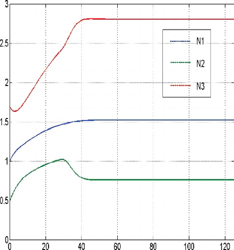
Here, for large initial values of the tumor cells population, the optimal solution structure confirms the principal structure of the corresponding non-constrained finite horizon control problem (cf. Schättler & Ledzewicz, 2015, p. 159), in the sense that maximal tolerated dosages of the cytotoxic agent at the beginning of the treatment are optimal. After some time they are gradually decreased to a constant medium level, compare Figures 1–3 and 4–6. Similar to Schättler and Ledzewicz (2015), the used time scale corresponds to the number of treatment days.

Figure 1. States for a sufficient large budget and initial state N(0) = (10, 10, 10).

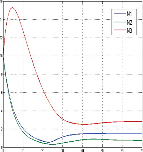
Figure 2. Controls for a sufficient large budget and initial state N(0) = (10, 10, 10).

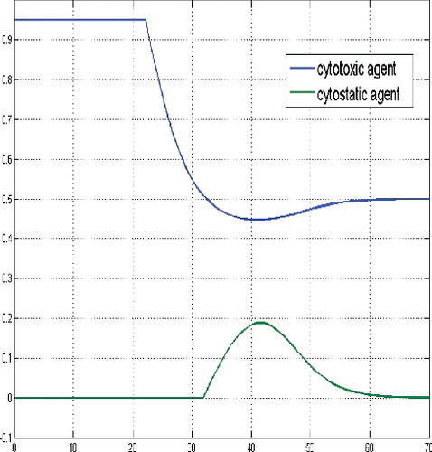
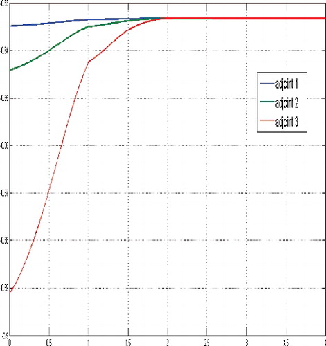
Figure 3. Adjoint functions for a sufficient large budget and initial state N(0) = (10, 10, 10).

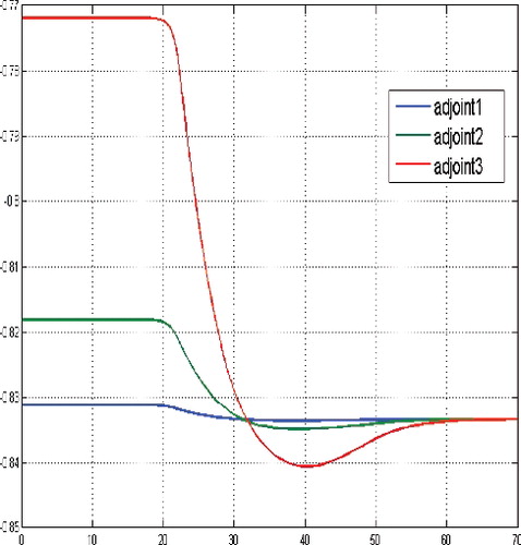
Figure 4. States for a sufficient large budget and large initial tumor cells population, i.e. N(0) = (30, 30, 30).

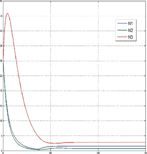
Figure 5. Controls for a sufficient large budget and large initial tumour cells population, i.e. N(0) = (30, 30, 30).

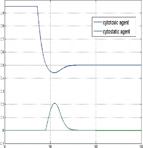
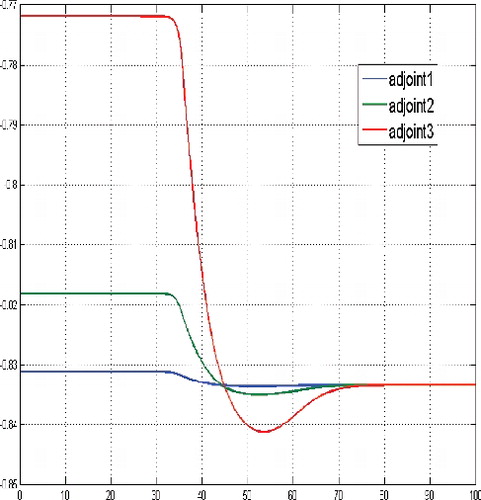
Figure 6. Adjoint functions for a sufficient large budget and large initial tumour cells population, i.e. N(0) = (30, 30, 30).

For small initial tumour cells population, e.g. for N(0) = (1, 1, 1), it also turns out to be optimal to control the system towards the same non-zero equilibrium, whose coordinates are partly even larger then the initial values, see Figures 7–9.

Figure 7. States for a sufficient large budget and N(0) = (1, 1, 1).

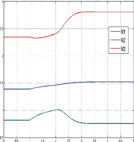
Figure 8. Controls for a sufficient large budget and N(0) = (1, 1, 1).

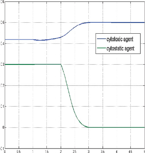
Figure 9. Adjoint functions for a sufficient large budget and N(0) = (1, 1, 1).

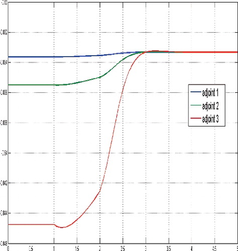
It can be explained by means of instability of the zero equilibrium of the uncontrolled system, though the zero equilibrium is more desirable from the medical point of view. However, in this case the dosage of the cytotoxic agent u(·) is growing very slowly up to a constant medium level. If the initial number of cancer cells belongs to a small neighbourhood of the non-zero equilibrium $\widehat{N}=({\widehat{N}}_1,{\widehat{N}}_2,{\widehat{N}}_3)$, e.g. N(0) = (3, 3, 3), then the non-zero phase of the cytostatic agent v(·) disappears, compare Figures 10–12.

Figure 10. States for a sufficient large budget and initial state near the equilibrium level, here N(0) = (3, 3, 3).

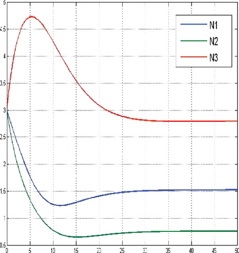
Figure 11. Controls for a sufficient large budget and and initial state near the equilibrium level, here N(0) = (3, 3, 3).

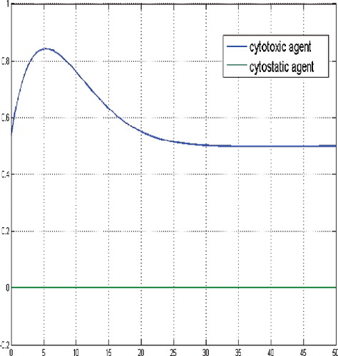
Figure 12. Adjoint functions for a sufficient large budget and and initial state near the equilibrium level, here N(0) = (3, 3, 3).

If the initial number of cancer cells is very low in comparison to the level of the non-zero equilibrium, e.g. N(0) = (0.3866, 0.1722, 0.4412) and cf. Figures 13–15, then the the structure of the optimal solution undergoes a significant change. It turns out to be optimal not to postpone the treatment but, starting with a very small dosage, to very slowly increase the dosage of cytotoxic therapeutic agent unless the number of cancer cells arrives approximately at the level of the equilibrium and afterwards to continue with a constant medium dosage.

Figure 13. States for a sufficient large budget and a small tumour cells population relatively compared to the level of the equilibrium, N(0) = (0.3866, 0.1722, 0.4412).

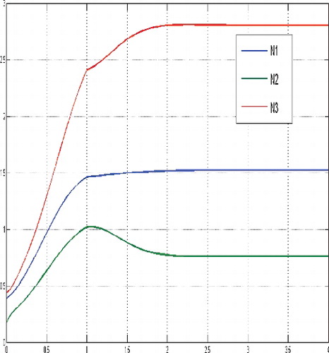
Figure 14. Controls for a sufficient large budget and a small tumour cells population relatively compared to the level of the equilibrium, N(0) = (0.3866, 0.1722, 0.4412).

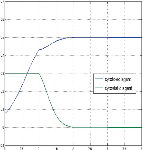
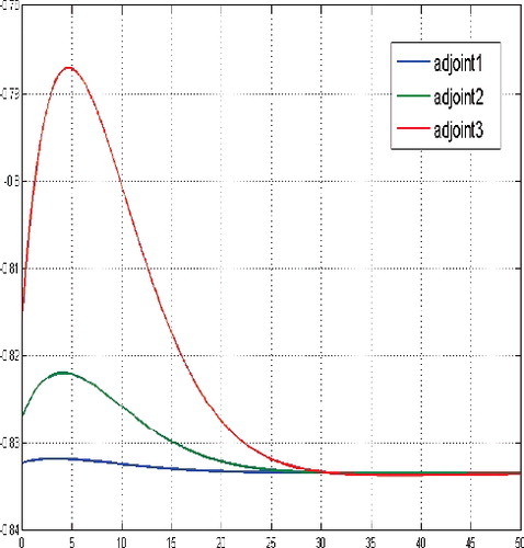
Figure 15. Adjoint functions for a sufficient large budget and a small tumor cells population relatively compared to the level of the equilibrium, N(0) = (0.3866, 0.1722, 0.4412).

Simultaneously, a shift of the non-zero phase of the cytostatic agent to the beginning of the treatment period and increasing of the dosage at the maximal level happens.

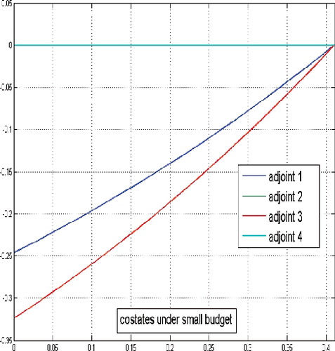
5.2 The case of a low ‘budget’ of therapeutics

In case of a small overall allowed amount of therapeutics d, the isoperimetrical constraint will become active at some finite point of time. It means that from this point of time on, both controls are identically zero over an infinite time interval and the system of cancer cells population starts uncontrolled growth. From Figures 16–18 it is obvious that the available amount of drugs is exhausted very fast and is not sufficient in order to bring the state trajectories in a small neighbourhood of the non-zero equilibrium level $\widehat{N}=({\widehat{N}}_1,{\widehat{N}}_2,{\widehat{N}}_3)$.

Figure 16. States for small budget d = 100 and N(0) = (10, 5, 10).

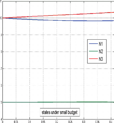
Figure 17. Controls for small budget d = 100 and N(0) = (10, 5, 10).

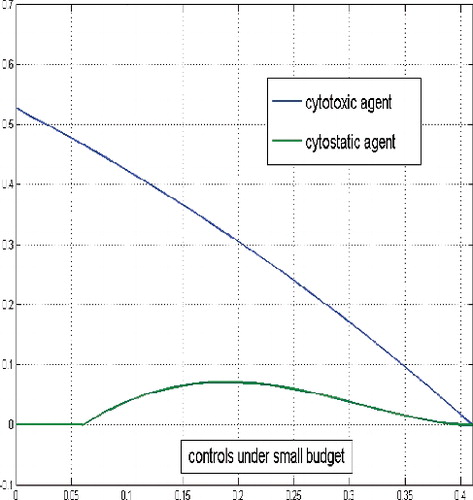
Figure 18. Costates for small budget d = 100 and N(0) = (10, 5, 10).

Remark 5.4:

Given a fixed initial state N(0) = (N ⁰ ₁, N ₂ ⁰, N ⁰ ₃), it is possible to find a minimal level of budget d _min which is necessary in order to have enough medical resources to control the system optimally towards the equilibrium over the whole infinite horizon. To do this, we need to compute the optimal controls for the ‘unconstrained’ cancer treatment problem and then set $$\begin{array}{c}\hfill d_{\text{min}}:=\underset{T\to \infty }{\lim \phantom{\mathrm{p}}}{N}_4\left(T\right)=\underset{T\to \infty }{\lim \phantom{\mathrm{p}}}\underset{0}{\overset{T}{\int }}(c_{1}u\left(t\right)+c_{2}v\left(t\right))e^{-\rho t}dt.\end{array}$$

5.3 The case of a threshold ‘budget‘’ of therapeutics

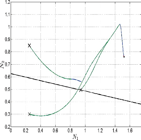
In the following phase diagrams which represent slice planes (N ₁ N ₂), (N ₂ N ₃) and (N ₁ N ₃) of the phase space (N ₁, N ₂, N ₃), cf. Figures 19–24 as well as Figure 25, the results are given for the budget d = 500. On all these pictures, the green line corresponds to the mode v(t) = v _max; the red line corresponds to the mode v(t) = v _min; the blue line denotes the mode, in which all controls are in the interior of the control set.

Figure 19.  Phase diagram, slice plane (N ₁,N ₂), case of the threshold budget (long path), d=500.

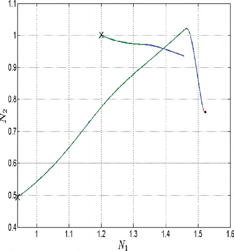
Figure 20.  Phase diagram, slice plane (N ₁,N ₃), case of the threshold budget (long path), d = 500 (long path), d = 500.

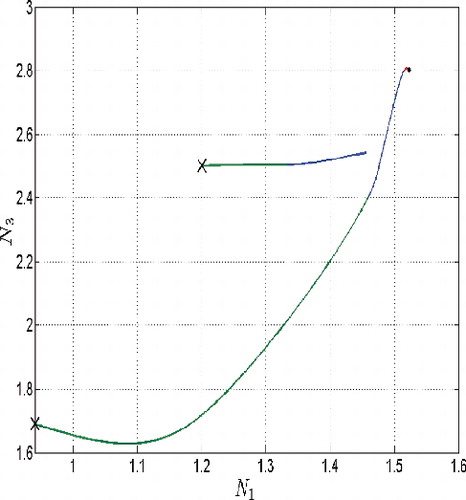
Figure 21. Phase diagra2, slice plane (N ₁,N ₃), case of the (long path), d = 500e threshold budget, d = 500.

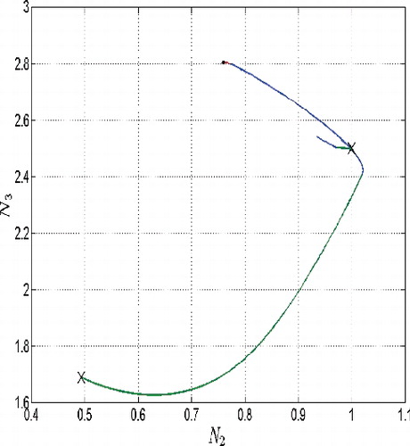
Figure 22.  Phase diagram, slice plane (N ₁,N ₂), case of budget constraint which does not become active (shorter path going near by the equilibrium), d = 500.

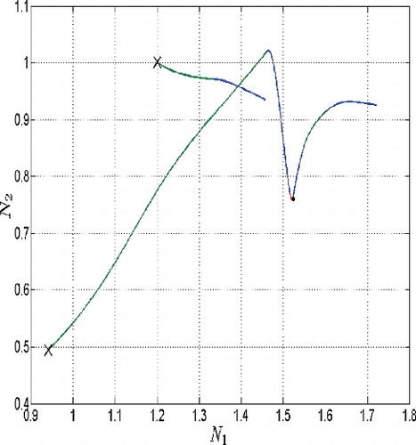
Figure 23.  Phase diagram, slice plane (N ₁,N ₃), case of budget constraint which does not become active (shorter path going near by the equilibrium), d = 500.

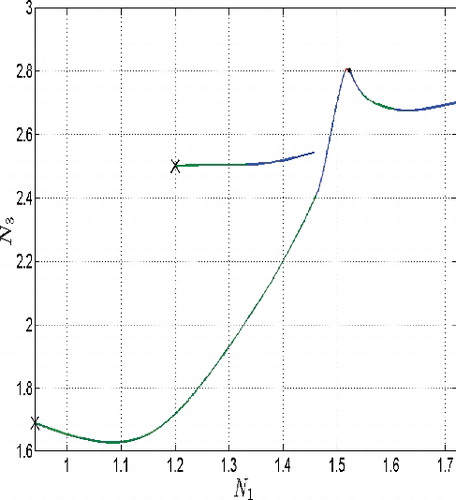
Figure 24.  Phase diagram, slice plane (N ₂,N ₃), case of budget constraint which does not become active (shorter path going near by the equilibrium), d = 500.

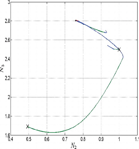
Figure 25. ‘Threshold state trajectories’ for budget d = 500.

The paths which lead to the equilibrium point, see long paths on Figures 19–21, satisfy the terminal constraint lim _{T → ∞} N ₄(T) = d, i.e. they correspond to the case of ‘budget’ d, which will be exhausted exactly in time T = ∞. The shorter paths on these images denote the paths corresponding to the case of the same budget d = 500 but which is exhausted in finite time. It means the initial value of the state is rather high compared to the value of the equilibrium so that the available amount of drugs is not sufficient to achieve the equilibrium. The paths are interrupted at that particular finite time, otherwise they would diverge what confirms the uncontrolled growth of the system of cancer cells.

The long paths connect the equilibrium with the initial point starting from which the set ‘budget’ d = 500 would be exhausted at exactly T = ∞. For solutions corresponding to the ‘threshold budget” compare Figures 26 and 27, and Figure 28.

Figure 26. ‘Threshold state trajectories’ for budget d = 500.

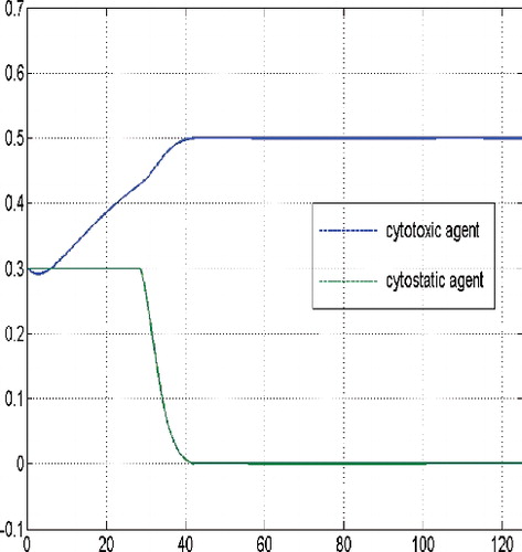
Figure 27. ‘Threshold adjoint functions’ for budget d = 500.

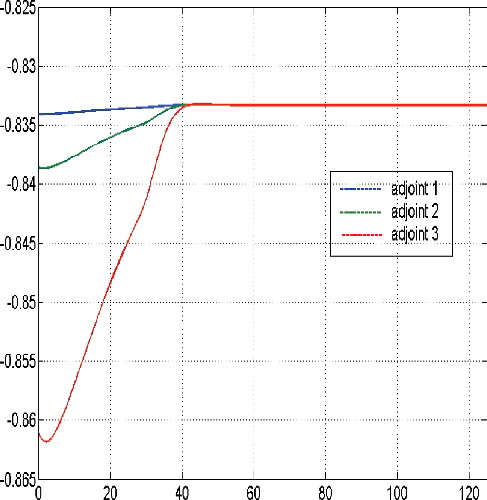
Figure 28. Growth of the budget variable N ₄ for budget d = 500.

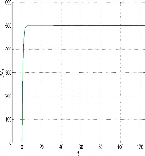
If the solution of the problem, where the isoperimetrical constraint becomes active after a finite time, approaches the initial state corresponding to the limiting condition lim _{T → ∞} N ₄(T) = d, then the corresponding path is getting closer to the equilibrium, cf. Figures 22–24. However, this path misses the equilibrium point and after passing nearby the equilibrium the trajectories drift away from it. Structurally, it means that for a fixed ‘budget’ amount d, there exists a surface in the state space (N ₁, N ₂, N ₃) which separates the initial states leading to the active budget constraint at some finite point of time from those initial states which lead to everywhere inactive isoperimetrical constraint. The surface itself contains all those initial states, for which the isoperimetrical constraint becomes active at exactly T = ∞, i.e. lim _{T → ∞} N ₄(T) = d. An exemplified slice curve, taken for a fixed value of N ₃ = 1 is given in Figure 29, black curve.

Figure 29. Slice curve for budget d = 500.

If the isoperimetrical constraint is not satisfied by the equilibrium $\widehat{N}=({\widehat{N}}_1,{\widehat{N}}_2,{\widehat{N}}_3)$ taken as the initial state, i.e. the optimal controls corresponding to this initial point induce the inequality lim _{T → ∞} N ₄(T) > d, then the separating surface will be located beyond the equilibrium point, cf. Figure 29. Otherwise, it lies above the equilibrium point. This picture shows also three paths, each of which corresponds to one of the cases presented in this discussion, namely a path starting exactly at the slice curve and corresponding to the ‘threshold case’, a path starting underneath the separating curve which flows into the ‘threshold’ path and corresponds to the case of sufficiently ‘high’ budget and a third shorter path starting above the separating curve and corresponding to the case of a budget which is exhausted in a finite time.

6. Conclusions

A class of infinite horizon optimal control problems with mixed control-state isoperimetrical constraint formulated in weighted Sobolev spaces was investigated, for which an existence theorem was derived. The proved theoretical result could have been successfully applied to an infinite horizon optimal control problem of cancer treatment by means of multi-drug chemotherapy. Based on the continuation algorithm for infinite horizon optimal control problems developed in Graß (2012), we also performed the numerical analysis for this model for different values of the ‘budget’ d. The most remarkable point resulting from the numerical analysis of the cancer treatment model with infinite horizon is that for small tumours, compared to the equilibrium level, it is optimal to gradually increase the dosage of the cytotoxic therapeutic agent up to a medium level which then should be held constant. In contrast to this, the corresponding finite horizon control problem implies already at the beginning of the treatment period the most tolerated dosage of the cytotoxic therapeutic agent. The future research focus will lie on extending the achieved results to the optimal control problems with highly nonlinear state equations and nonlinear isoperimetrical constraints. Considering more sophisticated cancer treatment models with infinite horizon including density functions resulting from the survival probability of a particular individual will also be a natural step in finding less aggressive long run cancer therapies.

Acknowledgments

The authors are very thankful to Prof. Vladimir Veliov for valuable discussions and suggestions for improving the manuscript. The authors acknowledge the TU Wien University Library for financial support through its Open Access Funding Program.

Disclosure statement

No potential conflict of interest was reported by the authors.

Additional information

Funding

Valeriya Lykina was supported by the German Research Foundation (DFG) [grant number LY 149/1-1].

Notes

1. This software package is available at http://orcos.tuwien.ac.at/research/ocmat_software/

References

- Aseev, S. , Besov, K. , & Kaniovski, S. (2013). The problem of optimal endogenous growth with exhaustible resources revisited. In J. Crespo Cuaresma et al. (Eds.), Green growth and sustainable development, dynamic modeling and econometrics in economics and finance (Vol. 14, pp. 3–30). Berlin Heidelberg: Springer-Verlag.
- Aseev, S. M. , & Kryazhimskii, A. V. (2007). The Pontryagin maximum principle and optimal economic growth problems. Proceedings of the Steklov Institute of Mathematics, 257 , 1–255.
- Aseev, S. M. , & Veliov, V. M. (2012). Maximum principle for problems with dominating discount. Dynamics of Continuous, Discrete and Impulsive Systems, Series B, 19 (1–2b), 43–63.
- Aseev, S. M. , & Veliov, V. M. (2014). Needle variations in infinite-horizon optimal control. Communications on Contemporary Mathematics, 619 (1–2b), 1–17.
- Aubin, J. P. , & Clarke, F. H. (1979). Shadow prices and duality for a class of optimal control problems. SIAM Journal on Control and Optimization, 17 (5), 567–586.
- Carlson, D. A. , Haurie, A. B. , & Leizarowitz, A . (1991). Infinite horizon optimal control . New York, NY: Springer-Verlag.
- Dunford, N. , & Schwartz, J. T. (1988). Linear operators. Part I: General theory . New York, NY: Wiley-Interscience.
- Elstrodt, J . (1996). Maß und integrationstheorie [Measure and integration theory] . Berlin: Springer.
- Feichtinger, G. , & Hartl, R. F . (1986). Optimale Kontrolle ökonomischer Prozesse [Optimal control of economic processes] . Berlin: de Gruyter.
- Garg, D. , Hager, W. W. , & Rao, A. V. (2011). Pseudospectral methods for solving infinite-horizon optimal control problems. Automatica, 47 , 829–837.
- Grass, D. , Caulkins, J. P. , Feichtinger, G. , Tragler, G. , & Behrens, D. A . (2008). Optimal control of nonlinear processes . Berlin: Springer.
- Graß, D. (2012). Numerical computation of the optimal vector field in a fishery model. Journal of Economic Dynamics and Control, 36 (10), 1626–1658.
- Halkin, H. (1979). Necessary conditions for optimal control problems with infinite horizons. Econometrica, 42 , 267–272.
- Kufner, A. (1985). Weighted Sobolev spaces . Chichester: Wiley.
- Kunkel, P. , & Von Dem Hagen, O. (2000). Numerical solution of infinite-horizon optimal-control problems. Computational Economics, 16 , 189–205.
- Ledzewicz, U. , Maurer, H. , & Schaettler, H. (2011). Optimal and suboptimal protocols for a mathematical model for tumor anti-angiogenesis in combination with chemotherapy. Mathematical Biosciences and Engineering, 8 (2), 307–323.
- Lykina, V. (2010). Beiträge zur Theorie der Optimalsteuerungsprobleme mit unendlichem Zeithorizont ( Dissertation). BTU Cottbus. Retrieved from http://opus.kobv.de/btu/volltexte/2010/1861/pdf/dissertationLykina.pdf
- Lykina, V. (2016). An existence theorem for a class of infinite horizon optimal control problems. Journal Optimization Theory and Applications, 69 (1), 50–73.
- Lykina, V. , & Pickenhain, S. (2016). Budget-constrained infinite horizon control problems with linear dynamics. In Proceedings of IEEE 55th Conference on Decision and Control, 12-14 Dec 2016. Las Vegas, USA.
- Lykina, V. , & Pickenhain, S. (2017). Weighted functional spaces approach in infinite horizon optimal control problems: A systematic analysis of hidden opportunities and advantages. Journal of Mathematical Analysis and Applications ( published online). doi:10.1016/j.jmaa.2017.04.069
- Lykina, V. , Pickenhain, S. , & Wagner, M. (2008). Different interpretations of the improper integral objective in an infinite horizon control problem. Mathematical Analysis and Applications, 340 , 498–510.
- Maurer, H. , & Pinho, M. d. R. (2015). Optimal control of epidemiological SEIR models with L 1 – objectives and control-state constraints. Pacific Journal of Optimization, 12 (2), 415–436.
- Pickenhain, S. (2010). On adequate transversality conditions for infinite horizon optimal control problems – A famous example of Halkin. In J. Crespo Cuaresma , T. Palokangas , & A. Tarasyev (Eds.), Dynamic systems, economic growth, and the environment: Dynamic modeling and econometrics in economics and finance (Vol. 12, pp. 3–22). Berlin: Springer.
- Pickenhain, S. , Burtchen, A. , Kolo, K , & Lykina, V. (2016). An indirect pseudospectral method for linear-quadratic infinite horizon optimal control problems. Optimization, 65 (3), 609–633.
- Pickenhain, S. , Lykina, V. , & Wagner, M. (2008). On the lower semicontinuity of functionals involving Lebesgue or improper Riemann integrals in infinite horizon optimal control problems. Control and Cybernetics, 37 (2), 451–468.
- Schättler, H. , & Ledzewicz, U . (2015). Optimal control for mathematical models of cancer therapies. An application of geometric methods. Interdisciplinary applied mathematics (Vol. 42). New York, NY: Springer.
- Tauchnitz, N. (2015). The pontryagin maximum principle for nonlinear infinite horizon optimal control problems with state constraints (pp. 1–75). Retrieved from https://arxiv.org/abs/1508.02340 .
- Torres, D. F. M. (2006). A Noether theorem on unimprovable conservation laws for vector-valued optimization problems in control theory. Georgian Mathematical Journal, 13 (1), 173–182.
- Yosida, K . (1974). Functional analysis . New York, Ny: Springer-Verlag.
- Zaslavski, A. J . (2006). Turnpike properties in the calculus of variations and optimal control. Heidelberg-New York-etc.: Springer.
- Zaslavski, A. J . (2014). Turnpike phenomenon and infinite horizon optimal control. Heidelberg-New York-etc: Springer.