New design methodology for adaptive switching gain based discrete-time sliding mode control

Abstract

The adaptive sliding mode control technique relaxes the assumption of known bound of the disturbance in discrete-time systems. However, the existing technique of gain adaptation in discrete-time sliding mode control has issues of gain overestimation and underestimation. Therefore, this paper proposes a technique to adapt the switching gain such that the adaptive gain can tackle the uncertainty without any knowledge of the bound of uncertainty while overcoming the over- and under-estimation problems of switching gain.

Keywords:

• Adaptive sliding mode
• discrete-time systems
• reaching law with adaptive gain
• unknown disturbance bound

1. Introduction

The sliding mode is well known robust control strategy which has many advantages such as invariance to matched parametric uncertainties/disturbance, simpler design technique, and system order-reduction (Alsmadi, Utkin, Haj-ahmed, & Xu, 2018; Bandyopadhyay & Janardhanan, 2005; Behera & Bandyopadhyay, 2016; Drakunov & Utkin, 1992; Draženović, 1969; Sharma & Janardhanan, 2017a; Utkin, 1977; Utkin & Poznyak, 2013). The recent developments and application of microcontrollers in the control circuitry has made the utilisation of discrete-time system representation more justifiable for controller design than continuous-time representation (Chakrabarty & Bandyopadhyay, 2016; Corradini, Cristofaro, & Orlando, 2014; Huber et al., 2016; Lincoln & Veres, 2010; Sharma & Janardhanan, 2017b; Yu, Wang, & Li, 2012). Furthermore, the application of sliding mode technology to control discrete-time systems like inventory management, flow control for connection-oriented communication networks, etc. has encouraged the studies on discrete-time sliding mode (DSM) (Bartoszewicz & Leéniewski, 2014, 2016; Sharma & Janardhanan, 2019). In the DSM control, the control input is calculated after a finite sampling interval and is held constant during this interval. Due to the finite sampling frequency, the system state trajectory may not move along but about the sliding surface, thus exhibiting quasi-sliding mode (QSM) (Gao, Wang, & Homaifa, 1995).

One of the methods of designing DSM is reaching law based approach (Bartoszewicz, 1998; Bartoszewicz & Latosiński, 2016; Chakrabarty & Bandyopadhyay, 2015; Du, Yu, Chen, & Li, 2016; Galias & Yu, 2008; Gao et al., 1995; Janardhanan & Kariwala, 2008; Singh, Sharma, & Janardhanan, 2017). The first idea was given by Gao et al. (1995) through defining the quasi-sliding mode and presenting a reaching law which guarantees the existence of defined quasi-sliding mode. The algorithm forces sliding function to reach the sliding surface in finite-time and then cross it after every sample. Bartoszewicz (1998) redefined the quasi-sliding mode and stated that the sliding function need not to cross sliding surface after every sample but only to remain around the sliding surface in a small band. Furthermore, various reaching laws have been proposed which claim lesser band width (Bartoszewicz & Latosiński, 2017, 2018; Du et al., 2016). However, these algorithms require prior the knowledge of the bound on the disturbance, which is not always plausible in practice (Bartoszewicz, 1998; Bartoszewicz & Latosiński, 2016, 2017, 2018; Bartoszewicz & Leéniewski, 2016; Chakrabarty & Bandyopadhyay, 2015; Du et al., 2016; Gao et al., 1995).

The adaptive sliding mode is a suitable design mechanism which aims to realise the benefits of a sliding mode design without any prior knowledge of bounds of the disturbance (Plestan, Shtessel, Brégeault, & Poznyak, 2010; Shtessel, Fridman, & Plestan, 2016). Among reaching law based DSM with adaptive gain techniques, the most popular technique is presented by Monsees and Scherpen (2002). This technique is well utilised in the recent literature (Vieira, Gastaldini, Azzolin, & Grundling, 2012; Xu, 2013). However, the adaptive switching gain suffers from the over- and under-estimation problems (Monsees & Scherpen, 2002). While the over-estimated switching gain produces unnecessary larger control input, the under-estimated gain compromises with the controller accuracy due to the lower value of applied gain than the required amount. Hence, it is imperative to design an adaptive DSM which can tackle the over- and under-estimation problems of switching gain.

1.1. Contribution

The major objective of this paper is to design an adaptive DSM controller which can

1. handle the bounded uncertainties/perturbation without any prior knowledge of the bound and

2. overcome the over- and under-estimation problems in estimated gain.

The organisation of the paper is as follows. After introduction in Section 1, the preliminaries of discrete-time sliding mode are given in Section 2. Features and drawbacks of the existing adaptive discrete-time sliding mode are also described in this Section. The main results of this paper are presented in Section 3. The simulation results and discussion in Section 4 are followed by conclusion in Section 5.

2. Preliminaries: discrete-time sliding mode

Consider an uncertain discrete-time LTI system (1) $x(k+1)=Ax\left(k\right)+Bu\left(k\right)+\tilde{d}\left(k\right),$(1) where $x\in {\mathbb{R}}^n$ is the state vector, $u\in \mathbb{R}$ is the control input and A, B are matrices of appropriate dimensions. The disturbance vector $\tilde{d}\left(k\right)\in {\mathbb{R}}^n$ represents the external disturbance effect in the system and satisfies the matching condition. The disturbance is unknown but assumed to be norm bounded. Let (2) $s\left(k\right)=cx\left(k\right)$(2) be the sliding function designed so that the system dynamics are stable when confined to the sliding surface $s\left(k\right)=0$ (Utkin, Guldner, & Shi, 2009). The effect of the disturbance vector $\tilde{d}\left(k\right)$ on the sliding function (2(2) $s\left(k\right)=cx\left(k\right)$(2) ) is defined as (3) $d\left(k\right)=c\tilde{d}\left(k\right).$(3) Since $\tilde{d}$ is assumed to be bounded, thus there exists a positive constant $\overline{d}$ such that (4) $|d\left(k\right)|\le \overline{d}.$(4) Gao et al. (1995) proposed a reaching law (5) $s(k+1)=(1-\phi )s\left(k\right)-ϵ\mathrm{s}\mathrm{g}\mathrm{n}\left(s\right(k\left)\right)+d\left(k\right),$(5) where $ϵ>0$ and $0<\phi <1$. If the gain is chosen such that (6) $ϵ>\frac{1+\phi }{1-\phi }\overline{d},$(6) then the reaching law (5(5) $s(k+1)=(1-\phi )s\left(k\right)-ϵ\mathrm{s}\mathrm{g}\mathrm{n}\left(s\right(k\left)\right)+d\left(k\right),$(5) ) guarantees the quasi-sliding mode in a band (7) $\mathrm{\Delta }=ϵ+\overline{d}.$(7) It can be noticed that the DSM band depends upon the switching gain ε; thus, lesser switching gain results in lesser band width, and consequently better accuracy. Nevertheless, one cannot make $ϵ=0$ as the sole purpose of ε is to tackle the disturbance d. Furthermore, if one selects a fixed value of ε from an estimated knowledge of $\overline{d}$, then the DSM band Δ increases. Consequently, better accuracy cannot be guaranteed. Thus, finding the exact $\overline{d}$ is difficult in practice and selection of high value of $\overline{d}$ may compel the controller to consume more control input as switching gain must satisfy (6(6) $ϵ>\frac{1+\phi }{1-\phi }\overline{d},$(6) ). Therefore, the challenge is to design ε in a way such that it can negotiate the uncertainties effectively and generate acceptable controller accuracy without consuming high control input.

2.1. Discrete-time sliding mode with adaptive switching gain

To remove the requirement of any prior knowledge of uncertainty bound, Monsees and Scherpen (2002) proposed DSM with adaptive switching gain. Given the uncertain system (1(1) $x(k+1)=Ax\left(k\right)+Bu\left(k\right)+\tilde{d}\left(k\right),$(1) ) and sliding function (2(2) $s\left(k\right)=cx\left(k\right)$(2) ) with the reaching law (8) $s(k+1)=(1-\phi )s\left(k\right)-ϵ\left(k\right)\mathrm{s}\mathrm{g}\mathrm{n}\left(s\right(k\left)\right)+d\left(k\right),$(8) where the switching gain is updated through the following adaptive law (Monsees & Scherpen, 2002) for a fixed scalar $\xi >0$: (9) $ϵ\left(k\right)=ϵ(k-1)+\xi \mathrm{s}\mathrm{g}\mathrm{n}\left(s\left(k\right)\right)\mathrm{s}\mathrm{g}\mathrm{n}\left(s(k-1)\right).$(9)

Observations: It can be noticed from the adaptive law (9(9) $ϵ\left(k\right)=ϵ(k-1)+\xi \mathrm{s}\mathrm{g}\mathrm{n}\left(s\left(k\right)\right)\mathrm{s}\mathrm{g}\mathrm{n}\left(s(k-1)\right).$(9) ) that the switching gain ε (i) only decreases if the sliding variable crosses the sliding surface and (ii) increases for all other cases. Based on these two scenarios, the following observations can be made:

1. The switching gain does not decrease even if the sliding function starts approaching toward the sliding surface; in fact, it keeps on increasing. This creates an over-estimation of switching gain and consequently produces unnecessary larger control input (as ε was sufficient to force the sliding function toward the sliding surface).

2. If the sliding function is gradually increasing and becoming unstable after crossing the sliding surface, the gain should be increasing to stabilise the system. On the contrary in this condition, the gain decreases following the adaptive law (9(9) $ϵ\left(k\right)=ϵ(k-1)+\xi \mathrm{s}\mathrm{g}\mathrm{n}\left(s\left(k\right)\right)\mathrm{s}\mathrm{g}\mathrm{n}\left(s(k-1)\right).$(9) ). This problem is known as gain underestimation and causes the poor performance, or the instability, of the system.

3. Furthermore, the rate of adaptation in (9(9) $ϵ\left(k\right)=ϵ(k-1)+\xi \mathrm{s}\mathrm{g}\mathrm{n}\left(s\left(k\right)\right)\mathrm{s}\mathrm{g}\mathrm{n}\left(s(k-1)\right).$(9) ) is constant.

Other than this, a time-varying gain is used in Salhi, Kamoun, Essounbouli, and Hamzaoui (2016) as (10) $ϵ\left(k\right)={\gamma }_0ϵ(k-1)+{\gamma }^0(1-{\gamma }_0),$(10) where $0<{\gamma }_0<1$ and $0<{\gamma }^0<1$ are termed as constant parameters.

Observations: The gain (10(10) $ϵ\left(k\right)={\gamma }_0ϵ(k-1)+{\gamma }^0(1-{\gamma }_0),$(10) ) used in Salhi et al. (2016) is an exponentially decreasing function of time (samples) and does not depend on the evaluations of sliding function. Consequently, the gain decreases even if the value of sliding function increases, giving rise to the problem of gain under-estimation.

2.2. Motivation

Considering the drawbacks of the existing algorithms, a new update law is to be designed such that:

1. The switching gain should start decreasing when the sliding function is approaching the sliding surface and vice-versa. Thus, this action will solve the problem of overestimation.

2. The switching gain should depend upon the sliding function, rather than only on the sign of the sliding function. This action will generate sufficient magnitude of the gain and the problem of gain underestimation will be solved.

3. The rate of adaptation should not be constant but varying and depend upon the sliding function. If the sliding function is far from the sliding surface, the rate of adaptation should be large and vice versa. This action will reduce the problem of choosing the optimal value of rate of adaptation.

Remark 2.1

It is important to note that the primary contribution of this paper is to propose a new gain adaptation law for discrete-time sliding mode that can alleviate the over- and under-estimation problems of switching gain. Furthermore, to justify the efficacy of the proposed scheme, it is compared with the existing adaptive discrete-time sliding mode controllers developed by Monsees and Scherpen (2002) and Salhi et al. (2016), both of which utilises the reaching law (8(8) $s(k+1)=(1-\phi )s\left(k\right)-ϵ\left(k\right)\mathrm{s}\mathrm{g}\mathrm{n}\left(s\right(k\left)\right)+d\left(k\right),$(8) ) proposed by Gao et al. (1995). Therefore, to keep parity in the comparison, the same reaching law is used in this paper and the subsequent theoretical analysis are also carried out accordingly. Nevertheless, there exist other various reaching laws with non-adaptive gains in the literature (Bartoszewicz & Latosiński, 2016, 2017, 2018; Du et al., 2016) with their respective advantages and disadvantages. Additional adoption of any of these reaching laws would demand a significant overhaul of the theoretical analysis. Hence, to maintain the flow of the paper more focused as well as parity in comparison, we have solely used the reaching law of Gao et al. (1995) and verification of the proposed gain adaptation law with other reaching laws is kept as future work.

3. Main results

A new gain adaptation law for the reaching law (8(8) $s(k+1)=(1-\phi )s\left(k\right)-ϵ\left(k\right)\mathrm{s}\mathrm{g}\mathrm{n}\left(s\right(k\left)\right)+d\left(k\right),$(8) ) is proposed as (11) $ϵ\left(k\right)=\mathrm{m}\mathrm{a}\mathrm{x}\left\{0,{ϵ}_m\left(k\right)\right\},\mathrm{\forall }k\ge 0,$(11) where (12) ${ϵ}_m\left(k\right)=\left\{\begin{array}{l}ϵ(k-1)+\gamma |s\left(k\right)|\mathrm{i}\mathrm{f}|\left\{s\right(k)|>|s(k-1\left)|\right\}\\ \mathrm{a}\mathrm{n}\mathrm{d}\left\{\text{sgn}\right[s\left(k\right)]=\text{sgn}[s(k-1)\left]\right\},\\ (1-\phi )|s\left(k\right)|\mathrm{i}\mathrm{f}\left\{|s\right(k)|>|s(k-1\left)|\right\}\\ \mathrm{a}\mathrm{n}\mathrm{d}\left\{\text{sgn}\right[s\left(k\right)]=-\text{sgn}[s(k-1)\left]\right\},\\ ϵ(k-1)-\beta |s\left(k\right)|\mathrm{i}\mathrm{f}|s\left(k\right)|\le |s(k-1)|.\end{array}\right.$(12) It can be noticed from the third law of (12(12) ${ϵ}_m\left(k\right)=\left\{\begin{array}{l}ϵ(k-1)+\gamma |s\left(k\right)|\mathrm{i}\mathrm{f}|\left\{s\right(k)|>|s(k-1\left)|\right\}\\ \mathrm{a}\mathrm{n}\mathrm{d}\left\{\text{sgn}\right[s\left(k\right)]=\text{sgn}[s(k-1)\left]\right\},\\ (1-\phi )|s\left(k\right)|\mathrm{i}\mathrm{f}\left\{|s\right(k)|>|s(k-1\left)|\right\}\\ \mathrm{a}\mathrm{n}\mathrm{d}\left\{\text{sgn}\right[s\left(k\right)]=-\text{sgn}[s(k-1)\left]\right\},\\ ϵ(k-1)-\beta |s\left(k\right)|\mathrm{i}\mathrm{f}|s\left(k\right)|\le |s(k-1)|.\end{array}\right.$(12) ) that ${ϵ}_m\left(k\right)$ decreases in this case; however, if ${ϵ}_m\left(k\right)$ attempts to be negative then, ε is kept at zero by virtue of the law (11(11) $ϵ\left(k\right)=\mathrm{m}\mathrm{a}\mathrm{x}\left\{0,{ϵ}_m\left(k\right)\right\},\mathrm{\forall }k\ge 0,$(11) ). This ensures the non-negativity of the gain ε. In other cases, $ϵ\left(k\right)={ϵ}_m\left(k\right)$. The constant design parameters γ and β can be tuned according to the required system performance; $ϵ\left(0\right)$ denotes the initial value of gain. It is important to study the boundedness of ε and has been carried out in Theorem 3.1.

Theorem 3.1

Given the reaching law (8(8) $s(k+1)=(1-\phi )s\left(k\right)-ϵ\left(k\right)\mathrm{s}\mathrm{g}\mathrm{n}\left(s\right(k\left)\right)+d\left(k\right),$(8) ) and switching gain adaptation law (12(12) ${ϵ}_m\left(k\right)=\left\{\begin{array}{l}ϵ(k-1)+\gamma |s\left(k\right)|\mathrm{i}\mathrm{f}|\left\{s\right(k)|>|s(k-1\left)|\right\}\\ \mathrm{a}\mathrm{n}\mathrm{d}\left\{\text{sgn}\right[s\left(k\right)]=\text{sgn}[s(k-1)\left]\right\},\\ (1-\phi )|s\left(k\right)|\mathrm{i}\mathrm{f}\left\{|s\right(k)|>|s(k-1\left)|\right\}\\ \mathrm{a}\mathrm{n}\mathrm{d}\left\{\text{sgn}\right[s\left(k\right)]=-\text{sgn}[s(k-1)\left]\right\},\\ ϵ(k-1)-\beta |s\left(k\right)|\mathrm{i}\mathrm{f}|s\left(k\right)|\le |s(k-1)|.\end{array}\right.$(12) ), there exists a ${ϵ}^{\ast }\in {\mathbb{R}}^{+}$ such that $ϵ\left(k\right)\le {ϵ}^{\ast }\mathrm{\forall }k\ge 0$.

Proof.

According to the adaptation law (12(12) ${ϵ}_m\left(k\right)=\left\{\begin{array}{l}ϵ(k-1)+\gamma |s\left(k\right)|\mathrm{i}\mathrm{f}|\left\{s\right(k)|>|s(k-1\left)|\right\}\\ \mathrm{a}\mathrm{n}\mathrm{d}\left\{\text{sgn}\right[s\left(k\right)]=\text{sgn}[s(k-1)\left]\right\},\\ (1-\phi )|s\left(k\right)|\mathrm{i}\mathrm{f}\left\{|s\right(k)|>|s(k-1\left)|\right\}\\ \mathrm{a}\mathrm{n}\mathrm{d}\left\{\text{sgn}\right[s\left(k\right)]=-\text{sgn}[s(k-1)\left]\right\},\\ ϵ(k-1)-\beta |s\left(k\right)|\mathrm{i}\mathrm{f}|s\left(k\right)|\le |s(k-1)|.\end{array}\right.$(12) ), the switching gain ε decreases for $|s\left(k\right)|\le |s(k-1)|$. Hence, the verification for the boundedness of ε for this scenario is not required. However, ε increases if $|s\left(k\right)|>|s(k-1)|$. Thus, to ensure boundedness of ε, only the condition $|s\left(k\right)|>|s(k-1)|$ is studied in the following cases:

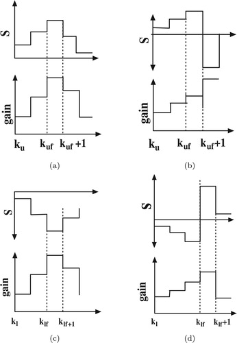
Case (1): $s\left(k\right),s(k-1)>0$

In this case, as shown in Figure 1(a), the sliding function is diverging away from the sliding surface. The value of the switching gain at any instant can be written as (13) $ϵ\left(k\right)=ϵ(k_u-1)+\gamma \sum _{i=k_u}^k|s\left(i\right)|,$(13) where $k_u$ denotes the time when Case (1) commences. Since $ϵ(k_u-1)\ge 0$, (13(13) $ϵ\left(k\right)=ϵ(k_u-1)+\gamma \sum _{i=k_u}^k|s\left(i\right)|,$(13) ) yields (14) $ϵ\left(k\right)\ge \gamma \sum _{i=k_u}^k|s\left(i\right)|.$(14) On considering the maximum disturbance in the positive half and the condition (14(14) $ϵ\left(k\right)\ge \gamma \sum _{i=k_u}^k|s\left(i\right)|.$(14) ), the sliding function at sample $(k+1)$ from (8(8) $s(k+1)=(1-\phi )s\left(k\right)-ϵ\left(k\right)\mathrm{s}\mathrm{g}\mathrm{n}\left(s\right(k\left)\right)+d\left(k\right),$(8) ) is obtained as (15) $s(k+1)\le (1-\phi )s\left(k\right)-\gamma \sum _{i=k_u}^k|s\left(i\right)|+\overline{d}.$(15) As $\overline{d}$ is a constant and ε increases with every sample, there exists a finite sample $k_{uf}$ such that (16) $\gamma \sum _{i=k_u}^{k_{uf}}|s\left(i\right)|-\overline{d}>0.$(16) Since $0<(1-\phi )<1$ and $s\left(k_{uf}\right)>0$ in Case (1), then substituting (16(16) $\gamma \sum _{i=k_u}^{k_{uf}}|s\left(i\right)|-\overline{d}>0.$(16) ) in (15(15) $s(k+1)\le (1-\phi )s\left(k\right)-\gamma \sum _{i=k_u}^k|s\left(i\right)|+\overline{d}.$(15) ), one has the at $k=k_{uf}$ (17) $s(k_{uf}+1)<(1-\phi )s\left(k_{uf}\right)<|s\left(k_{uf}\right)|.$(17) If $s(k_{uf}+1)\ge 0$, then (17(17) $s(k_{uf}+1)<(1-\phi )s\left(k_{uf}\right)<|s\left(k_{uf}\right)|.$(17) ) implies $|s\left(k\right)|<|s(k-1)|$ at $k=k_{uf}+1$. In this situation, $ϵ\left(k\right)$ decreases according to the third law of (12(12) ${ϵ}_m\left(k\right)=\left\{\begin{array}{l}ϵ(k-1)+\gamma |s\left(k\right)|\mathrm{i}\mathrm{f}|\left\{s\right(k)|>|s(k-1\left)|\right\}\\ \mathrm{a}\mathrm{n}\mathrm{d}\left\{\text{sgn}\right[s\left(k\right)]=\text{sgn}[s(k-1)\left]\right\},\\ (1-\phi )|s\left(k\right)|\mathrm{i}\mathrm{f}\left\{|s\right(k)|>|s(k-1\left)|\right\}\\ \mathrm{a}\mathrm{n}\mathrm{d}\left\{\text{sgn}\right[s\left(k\right)]=-\text{sgn}[s(k-1)\left]\right\},\\ ϵ(k-1)-\beta |s\left(k\right)|\mathrm{i}\mathrm{f}|s\left(k\right)|\le |s(k-1)|.\end{array}\right.$(12) ). Otherwise, if $s(k_{uf}+1)<0$, then there exist two possibilities at $k=k_{uf}+1$:

Figure 1. Possible conditions of adaptive sliding mode. (a) Case-1. (b) Case-2. (c) Case-3. (d) Case-4.

1. If $|s\left(k\right)|\le |s(k-1)|$, then $ϵ\left(k\right)$ decreases as mentioned earlier.

2. If $|s\left(k\right)|>|s(k-1)|$, then $s\left(k\right)<0,s(k-1)>0$, as shown in Figure 1(b). The dynamics of s and boundedness for ε for this situation is studied in Case (2).

Case (2): $s(k-1)>0,s\left(k\right)<0$

In this case, the gain is updated through the second law of (12(12) ${ϵ}_m\left(k\right)=\left\{\begin{array}{l}ϵ(k-1)+\gamma |s\left(k\right)|\mathrm{i}\mathrm{f}|\left\{s\right(k)|>|s(k-1\left)|\right\}\\ \mathrm{a}\mathrm{n}\mathrm{d}\left\{\text{sgn}\right[s\left(k\right)]=\text{sgn}[s(k-1)\left]\right\},\\ (1-\phi )|s\left(k\right)|\mathrm{i}\mathrm{f}\left\{|s\right(k)|>|s(k-1\left)|\right\}\\ \mathrm{a}\mathrm{n}\mathrm{d}\left\{\text{sgn}\right[s\left(k\right)]=-\text{sgn}[s(k-1)\left]\right\},\\ ϵ(k-1)-\beta |s\left(k\right)|\mathrm{i}\mathrm{f}|s\left(k\right)|\le |s(k-1)|.\end{array}\right.$(12) ) as (18) $ϵ\left(k\right)=(1-\phi )|s\left(k\right)|.$(18) On using the gain value in the reaching law (8(8) $s(k+1)=(1-\phi )s\left(k\right)-ϵ\left(k\right)\mathrm{s}\mathrm{g}\mathrm{n}\left(s\right(k\left)\right)+d\left(k\right),$(8) ) and (18(18) $ϵ\left(k\right)=(1-\phi )|s\left(k\right)|.$(18) ), the sliding function is obtained to be $s(k+1)=-(1-\phi )|s\left(k\right)|+(1-\phi )|s\left(k\right)|+d\left(k\right).$ Since $d\left(k\right)$ is bounded, the sliding function also remains bounded as $|s(k+1)|\le \overline{d}.$ In this case, ε only depends upon the instantaneous value of sliding function. Thus, ε is also bounded for this case.

It is mentioned in the Case (1), that at a finite time $k=k_{uf}+1$, either $ϵ\left(k\right)$ decreases or the dynamics of $s\left(k\right)$ follows Case (2). Thereafter, it is shown that $ϵ\left(k\right)$ remains bounded in Case (2) by virtue of the adaptive law (12(12) ${ϵ}_m\left(k\right)=\left\{\begin{array}{l}ϵ(k-1)+\gamma |s\left(k\right)|\mathrm{i}\mathrm{f}|\left\{s\right(k)|>|s(k-1\left)|\right\}\\ \mathrm{a}\mathrm{n}\mathrm{d}\left\{\text{sgn}\right[s\left(k\right)]=\text{sgn}[s(k-1)\left]\right\},\\ (1-\phi )|s\left(k\right)|\mathrm{i}\mathrm{f}\left\{|s\right(k)|>|s(k-1\left)|\right\}\\ \mathrm{a}\mathrm{n}\mathrm{d}\left\{\text{sgn}\right[s\left(k\right)]=-\text{sgn}[s(k-1)\left]\right\},\\ ϵ(k-1)-\beta |s\left(k\right)|\mathrm{i}\mathrm{f}|s\left(k\right)|\le |s(k-1)|.\end{array}\right.$(12) ). Hence, on combining the results obtained from Case (1) and Case (2), it can be inferred that $\mathrm{\exists }{ϵ}_u^{\ast }\in {\mathbb{R}}^{+}$ such that $ϵ\left(k\right)\le {ϵ}_u^{\ast }$ for both the Cases (1) and (2).

Case (3): $s\left(k\right),s(k-1)<0$

In this case, as shown in Figure 1(c), $|s|$ increases with s being in the negative plane. In this case, the gain is updated through the first law of (12(12) ${ϵ}_m\left(k\right)=\left\{\begin{array}{l}ϵ(k-1)+\gamma |s\left(k\right)|\mathrm{i}\mathrm{f}|\left\{s\right(k)|>|s(k-1\left)|\right\}\\ \mathrm{a}\mathrm{n}\mathrm{d}\left\{\text{sgn}\right[s\left(k\right)]=\text{sgn}[s(k-1)\left]\right\},\\ (1-\phi )|s\left(k\right)|\mathrm{i}\mathrm{f}\left\{|s\right(k)|>|s(k-1\left)|\right\}\\ \mathrm{a}\mathrm{n}\mathrm{d}\left\{\text{sgn}\right[s\left(k\right)]=-\text{sgn}[s(k-1)\left]\right\},\\ ϵ(k-1)-\beta |s\left(k\right)|\mathrm{i}\mathrm{f}|s\left(k\right)|\le |s(k-1)|.\end{array}\right.$(12) ). The value of gain at sample k is (19) $ϵ\left(k\right)=ϵ(k_l-1)+\gamma \sum _{i=k_l}^k|s\left(i\right)|,$(19) where $k_l$ denotes the time when Case (3) starts. Since $ϵ(k_l-1)\ge 0$, (19(19) $ϵ\left(k\right)=ϵ(k_l-1)+\gamma \sum _{i=k_l}^k|s\left(i\right)|,$(19) ) yields (20) $ϵ\left(k\right)\ge \gamma \sum _{i=k_l}^k|s\left(i\right)|.$(20) On considering the worst case of disturbance in the negative half of plane and using (20(20) $ϵ\left(k\right)\ge \gamma \sum _{i=k_l}^k|s\left(i\right)|.$(20) ), the sliding function at sample $(k+1)$ is obtained from (8(8) $s(k+1)=(1-\phi )s\left(k\right)-ϵ\left(k\right)\mathrm{s}\mathrm{g}\mathrm{n}\left(s\right(k\left)\right)+d\left(k\right),$(8) ) as (21) $s(k+1)\ge -(1-\phi )|s\left(k\right)|+\gamma \sum _{i=k_l}^k|s\left(i\right)|-\overline{d}.$(21) Since $\overline{d}$ is constant and ε increases with every sample, there exists a finite sample $k_{lf}$ such that (22) $\gamma \sum _{i=k_l}^{k_{lf}}|s\left(i\right)|-\overline{d}>0.$(22) Since $0<(1-\phi )<1$, using (21(21) $s(k+1)\ge -(1-\phi )|s\left(k\right)|+\gamma \sum _{i=k_l}^k|s\left(i\right)|-\overline{d}.$(21) )–(22(22) $\gamma \sum _{i=k_l}^{k_{lf}}|s\left(i\right)|-\overline{d}>0.$(22) ), we have the following at $k=k_{lf}$ (23) $s(k_{lf}+1)>-(1-\phi )|s\left(k_{lf}\right)|>-|s\left(k_{lf}\right)|.$(23) The condition (23(23) $s(k_{lf}+1)>-(1-\phi )|s\left(k_{lf}\right)|>-|s\left(k_{lf}\right)|.$(23) ) implies that the sliding function stops increasing in the negative direction of the sliding surface at $k=k_{lf}+1$. If $s(k_{lf}+1)\le 0$ then the condition $|s\left(k\right)|\le |s(k-1)|$ is satisfied, which prompts ε to decrease according to the third law of (12(12) ${ϵ}_m\left(k\right)=\left\{\begin{array}{l}ϵ(k-1)+\gamma |s\left(k\right)|\mathrm{i}\mathrm{f}|\left\{s\right(k)|>|s(k-1\left)|\right\}\\ \mathrm{a}\mathrm{n}\mathrm{d}\left\{\text{sgn}\right[s\left(k\right)]=\text{sgn}[s(k-1)\left]\right\},\\ (1-\phi )|s\left(k\right)|\mathrm{i}\mathrm{f}\left\{|s\right(k)|>|s(k-1\left)|\right\}\\ \mathrm{a}\mathrm{n}\mathrm{d}\left\{\text{sgn}\right[s\left(k\right)]=-\text{sgn}[s(k-1)\left]\right\},\\ ϵ(k-1)-\beta |s\left(k\right)|\mathrm{i}\mathrm{f}|s\left(k\right)|\le |s(k-1)|.\end{array}\right.$(12) ). Otherwise, if $s(k_{lf}+1)>0$ then there exist two possibilities at $k=k_{lf}+1$:

1. If $|s\left(k\right)|\le |s(k-1)|$, then $ϵ\left(k\right)$ decreases as mentioned earlier.

2. If $|s\left(k\right)|>|s(k-1)|$, then we have $s\left(k\right)<0,s(k-1)>0$ at $k=k_{lf}+1$, as shown in Figure 1(d). The dynamics of $s\left(k\right)$ and boundedness for ε for this situation is studied subsequently in Case (4).

Case (4): $s(k-1)<0,s\left(k\right)>0$

In this case, the gain is updated through the second law of (12(12) ${ϵ}_m\left(k\right)=\left\{\begin{array}{l}ϵ(k-1)+\gamma |s\left(k\right)|\mathrm{i}\mathrm{f}|\left\{s\right(k)|>|s(k-1\left)|\right\}\\ \mathrm{a}\mathrm{n}\mathrm{d}\left\{\text{sgn}\right[s\left(k\right)]=\text{sgn}[s(k-1)\left]\right\},\\ (1-\phi )|s\left(k\right)|\mathrm{i}\mathrm{f}\left\{|s\right(k)|>|s(k-1\left)|\right\}\\ \mathrm{a}\mathrm{n}\mathrm{d}\left\{\text{sgn}\right[s\left(k\right)]=-\text{sgn}[s(k-1)\left]\right\},\\ ϵ(k-1)-\beta |s\left(k\right)|\mathrm{i}\mathrm{f}|s\left(k\right)|\le |s(k-1)|.\end{array}\right.$(12) ). The value of gain in this case is $ϵ\left(k\right)=(1-\phi )|s\left(k\right)|.$ Similar to the argument made in Case (2), s and consequently ε remain bounded.

On combining Case (3) and Case (4), it can be inferred that there exists an ${ϵ}_l^{\ast }\in {\mathbb{R}}^{+}$ such that $ϵ\left(k\right)\le {ϵ}_l^{\ast }$ for both these two cases. Observing the boundedness conditions of all the individual possible cases, it can be inferred that $ϵ\left(k\right)\le {ϵ}^{\ast }\mathrm{\forall }k\ge 0\mathrm{w}\mathrm{h}\mathrm{e}\mathrm{r}\mathrm{e}{ϵ}^{\ast }=max\{{ϵ}_u^{\ast },{ϵ}_l^{\ast }\}.$

Theorem 3.2

The reaching law (8(8) $s(k+1)=(1-\phi )s\left(k\right)-ϵ\left(k\right)\mathrm{s}\mathrm{g}\mathrm{n}\left(s\right(k\left)\right)+d\left(k\right),$(8) ) with the gain adaptation law (12(12) ${ϵ}_m\left(k\right)=\left\{\begin{array}{l}ϵ(k-1)+\gamma |s\left(k\right)|\mathrm{i}\mathrm{f}|\left\{s\right(k)|>|s(k-1\left)|\right\}\\ \mathrm{a}\mathrm{n}\mathrm{d}\left\{\text{sgn}\right[s\left(k\right)]=\text{sgn}[s(k-1)\left]\right\},\\ (1-\phi )|s\left(k\right)|\mathrm{i}\mathrm{f}\left\{|s\right(k)|>|s(k-1\left)|\right\}\\ \mathrm{a}\mathrm{n}\mathrm{d}\left\{\text{sgn}\right[s\left(k\right)]=-\text{sgn}[s(k-1)\left]\right\},\\ ϵ(k-1)-\beta |s\left(k\right)|\mathrm{i}\mathrm{f}|s\left(k\right)|\le |s(k-1)|.\end{array}\right.$(12) ) has a Globally Ultimately Bounded solution and the sliding function is ultimately bounded in a band $|s\left(k\right)|\le \frac{{ϵ}^{\ast }+\overline{d}}{\phi }.$

Proof.

The ultimate boundedness of the sliding function can be proved by the Lyapunov-like stability analysis. Consider a Lyapunov candidate function $V\left(k\right)=\alpha |s\left(k\right)|,$ where α is a positive constant. The first difference of the Lyapunov function can be obtained to be (24) $\begin{array}{rl}\mathrm{△}V\left(k\right)& =V(k+1)-V\left(k\right)\\ & =\alpha |s(k+1)|-\alpha |s\left(k\right)|.\end{array}$(24) Let $g\left(k\right)=-ϵ\left(k\right)\mathrm{s}\mathrm{g}\mathrm{n}\left(s\right(k\left)\right)+d\left(k\right)$, then on using (8(8) $s(k+1)=(1-\phi )s\left(k\right)-ϵ\left(k\right)\mathrm{s}\mathrm{g}\mathrm{n}\left(s\right(k\left)\right)+d\left(k\right),$(8) ) in (24(24) $\begin{array}{rl}\mathrm{△}V\left(k\right)& =V(k+1)-V\left(k\right)\\ & =\alpha |s(k+1)|-\alpha |s\left(k\right)|.\end{array}$(24) ) yields (25) $\mathrm{△}V\left(k\right)=\alpha |(1-\phi )s\left(k\right)+g\left(k\right)|-\alpha |s\left(k\right)|.$(25) Since $0<(1-\phi )<1$, (25(25) $\mathrm{△}V\left(k\right)=\alpha |(1-\phi )s\left(k\right)+g\left(k\right)|-\alpha |s\left(k\right)|.$(25) ) leads to (26) $\begin{array}{rl}\mathrm{△}V\left(k\right)& \le \alpha (1-\phi )|s\left(k\right)|+\alpha |g\left(k\right)|-\alpha |s\left(k\right)|\\ & \le -\alpha \phi |s\left(k\right)|+\alpha |g\left(k\right)|\\ & \le -\phi V\left(k\right)+\alpha |g\left(k\right)|.\end{array}$(26) Since $|g\left(k\right)|=|-ϵ\left(k\right)\mathrm{s}\mathrm{g}\mathrm{n}\left(s\right(k\left)\right)+d\left(k\right)|,$ with $ϵ\left(k\right)\le {ϵ}^{\ast }$ from Theorem (3.1), and the fact $|d\left(k\right)|\le \overline{d}$, the following relation holds: (27) $|g\left(k\right)|\le {ϵ}^{\ast }+\overline{d}.$(27) Then, using (27(27) $|g\left(k\right)|\le {ϵ}^{\ast }+\overline{d}.$(27) ), the following can be obtained from (26(26) $\begin{array}{rl}\mathrm{△}V\left(k\right)& \le \alpha (1-\phi )|s\left(k\right)|+\alpha |g\left(k\right)|-\alpha |s\left(k\right)|\\ & \le -\alpha \phi |s\left(k\right)|+\alpha |g\left(k\right)|\\ & \le -\phi V\left(k\right)+\alpha |g\left(k\right)|.\end{array}$(26) ) $\mathrm{△}V\left(k\right)\le -\phi V\left(k\right)+\alpha ({ϵ}^{\ast }+\overline{d}).$ Since $0<\phi <1$, the reaching law (8(8) $s(k+1)=(1-\phi )s\left(k\right)-ϵ\left(k\right)\mathrm{s}\mathrm{g}\mathrm{n}\left(s\right(k\left)\right)+d\left(k\right),$(8) ) has a Globally Ultimately Bounded solution and simultaneously, the ultimate band of the sliding function can be found to be $|s|\le \frac{{ϵ}^{\ast }+\overline{d}}{\phi }.$

4. Simulation results and comparison

In this section, the performance of the proposed algorithm is verified in comparison with the existing algorithms proposed by Monsees and Scherpen (2002) and Salhi et al. (2016), using two numerical examples. While the first example considers a rectilinear plant comprising of mass–damper–spring system, a CNC milling machine is considered as the second example. These complex models are chosen to support the theoretical findings.

4.1. Numerical simulation 1: Rectilinear plant

A rectilinear plant, as shown in Figure 2, is a electromechanical mass–spring–damper system which represents many industrial physical systems and can be represented by second order discrete-time equation (1(1) $x(k+1)=Ax\left(k\right)+Bu\left(k\right)+\tilde{d}\left(k\right),$(1) ) with parameters $A=\left[\begin{array}{cc}0& 1\\ -1& -0.1215\end{array}\right]$ and $b=\left[\begin{array}{c}0\\ 1\end{array}\right]$. The parameter c in (2(2) $s\left(k\right)=cx\left(k\right)$(2) ) is chosen to be $\left[12\right]$ and initial condition $x_0=[1010{]}^{\mathrm{T}}$. The other control parameters are given in Table 1. A disturbance signal $d_x\left(k\right)=[00.5{]}^{\mathrm{T}}\times (\mathrm{s}\mathrm{i}\mathrm{n}\left(k\right)+\mathrm{s}\mathrm{i}\mathrm{n}\left(k/3\right))$ is added to the system to imitate more realistic situation. The numerical example is simulated for 25 samples. To compare the performance of the proposed adaptation law, the same system is simulated using the adaptation law presented by Monsees and Scherpen (2002) with same the initial parameters.

The simulation results are presented in Figure 3. Quantitative measures of comparison, the absolute sum of switching gain $\sum _k|ϵ\left(k\right)|$ and absolute sum of control input $\sum _k|u\left(k\right)|$ are given in Table 2. As shown in Figure 3(a), the switching gain of the proposed controller is far lesser than that of the proposed by Monsees and Scherpen (2002). Furthermore, it can be observed in Table 2 that the absolute sum of gain on using Monsees and Scherpen (2002) and Salhi et al. (2016) are 30.4 and 19.2, respectively, while on using the proposed scheme it is found to be 4.3. Hence, the absolute sum of gain on using control algorithms of Monsees and Scherpen (2002) and Salhi et al. (2016) are more than 7 times and 4 times, respectively, than the proposed law. As a result of the lesser value of the adaptive gain, the control efforts in the proposed algorithm is about $28\mathrm{\%}$ lesser than control efforts using Monsees and Scherpen (2002). The control input is shown in Figure 3(b). Therefore, it can be noticed that the proposed scheme resolves the problem of gain overestimation.

Figure 2. Free body diagram of mass–spring system.

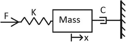
Figure 3. Simulation results of rectilinear plant. (a) Switching gain. (b) Control input. (c) Sliding function. (d) State $x_1$.

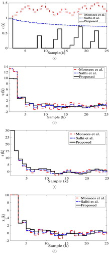
Table 1. Parameter values in simulation 1.

Sl.no	Parameter	Value
1	φ	0.5
2	β	1
3	ξ	0.1
4	γ	0.2

Table 2. Comparison of performance in simulation 1.

Sl.no	Control algorithm	$\sum _k\left|ϵ\right(k\left)\right|$	$\sum _k\left|u\right(k\left)\right|$
1	Existing adaptive law (Monsees & Scherpen, 2002)	30.4	45.5
2	Existing adaptive law (Salhi et al., 2016)	19.2	38.7
3	Proposed adaptive law	4.3	33.6

The sliding function, depicted in Figure 3(c), gradually reaches and then remains in the vicinity of the origin. Similarly, the system state, as seen inFigure 3(d), using the proposed algorithm remains in the vicinity of the origin.

Thus, the proposed adaptive sliding mode control algorithm guarantees lesser control efforts and better robustness as compared to the existing adaptive algorithm.

4.2. Numerical simulation 2: CNC milling machine

A model of CNC milling machine is provided by Eun, Kim, Kim, and Cho (1999). In this model, CNC servopack and motor are considered as a single plant. For further details of modelling and the value of physical parameters, the interested readers may refer Eun et al. (1999). This model is represented by second order discrete-time equation (1(1) $x(k+1)=Ax\left(k\right)+Bu\left(k\right)+\tilde{d}\left(k\right),$(1) ) with parameters $A=\left[\begin{array}{cc}1& 0.0006\\ 0& 0.3074\end{array}\right]$ and $B=\left[\begin{array}{c}0.0004\\ 0.6926\end{array}\right]$. The parameter c in (2(2) $s\left(k\right)=cx\left(k\right)$(2) ) is chosen to be $\left[2011\right]$ and initial condition $x_0=[11{]}^{\mathrm{T}}$. The other control parameters are given in Table 3. A disturbance signal $d_x\left(k\right)=[00.6926{]}^{\mathrm{T}}\times (\mathrm{s}\mathrm{i}\mathrm{n}\left(k\right))$ is added to the system to imitate more realistic situation. The numerical example is simulated for 100 samples.

Table 3. Parameter values in simulation 2.

Sl.no	Parameter	Value
1	φ	0.5
2	β	1
3	ξ	0.1
4	γ	0.2
5	${\gamma }_0$	0.8
6	${\gamma }^0$	0.6

The comparative simulation results for the CNC milling machine are presented in Figure 4. Similar to simulation 1, quantitative measures of comparison, the absolute sum of switching gain $\sum _k|ϵ\left(k\right)|$ and absolute sum of control input $\sum _k|u\left(k\right)|$ are given in Table 4. As shown in Figure 4(a), on using control algorithm of Salhi et al. (2016), the gain ε exponentially decreases irrespective of the evaluation of the sliding function. Therefore, it suffers from gain under-estimation. Although, the control algorithm given in Monsees and Scherpen (2002) allows ε to increase several times, but it still has high gain compared to the proposed adaptive law-based gain. The proposed algorithm enables ε to overcome the gain over- and under-estimation problems by following the evolutions of the sliding function. The control input for all the algorithms are shown in Figure 4(b). It can further be observed from Table 4 that the absolute sum of gain on using Monsees and Scherpen (2002) and Salhi et al. (2016) are 52.9 and 61.0, respectively. On the other hand, on using the proposed scheme, the absolute sum of gain is only 21.5. This observation also justifies the superiority of the proposed control law. The control effort in the proposed algorithm is also found to be lesser than that of Monsees and Scherpen (2002) and Salhi et al. (2016), owing to its lesser value of the adaptive gain.

Figure 4. Simulation results of CNC milling machine. (a) Switching gain. (b) Control input. (c) Sliding function. (d) State $x_1$.

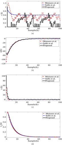
Table 4. Comparison of performance in simulation 2.

Sl.no	Control algorithm	$\sum _k\left|ϵ\right(k\left)\right|$	$\sum _k\left|u\right(k\left)\right|$
1	Existing adaptive law (Monsees & Scherpen, 2002)	52.9	1032.7
2	Existing adaptive law (Salhi et al., 2016)	61.0	1031.8
3	Proposed adaptive law	21.5	1009.8

5. Conclusion

An improved gain update law for adaptive discrete-time sliding mode has been proposed in this paper. The new gain adaptation law circumvents the problem of over- and under-estimation. The theoretical and subsequent simulation results further substantiate the advantages of the proposed scheme in terms of better robustness and lesser control efforts compared to the existing methods.

Disclosure statement

No potential conflict of interest was reported by the authors.

ORCID

Nalin Kumar Sharma  http://orcid.org/0000-0001-7494-757X

Spandan Roy  http://orcid.org/0000-0002-2238-9542

S. Janardhanan  http://orcid.org/0000-0003-3678-6300

References

- Alsmadi, Y. M., Utkin, V., Haj-ahmed, M. A., & Xu, L. (2018). Sliding mode control of power converters: DC/DC converters. International Journal of Control, 91(11), 2472–2493. doi: 10.1080/00207179.2017.1306112
- Bandyopadhyay, B., & Janardhanan, S. (2005). Discrete-time sliding mode control: A multirate-output feedback approach. Lecture notes in control and information sciences (Vol. 323). Berlin: Springer-Verlag.
- Bartoszewicz, A. (1998). Discrete-time quasi-sliding-mode control strategies. IEEE Transactions on Industrial Electronics, 45(4), 633–637. doi: 10.1109/41.704892
- Bartoszewicz, A., & Latosiński, P. (2016). Discrete time sliding mode control with reduced switching: A new reaching law approach. International Journal of Robust and Nonlinear Control, 26(1), 47–68. doi: 10.1002/rnc.3291
- Bartoszewicz, A., & Latosiński, P. (2017). Reaching law for DSMC systems with relative degree 2 switching variable. International Journal of Control, 90(8), 1626–1638. doi: 10.1080/00207179.2016.1216606
- Bartoszewicz, A., & Latosiński, P. (2018). Generalization of Gao's reaching law for higher relative degree sliding variables. IEEE Transactions on Automatic Control, 63(9), 3173–3179. doi: 10.1109/TAC.2018.2797193
- Bartoszewicz, A., & Leéniewski, P. (2014). Reaching law approach to the sliding mode control of periodic review inventory systems. IEEE Transactions on Automation Science and Engineering, 11(3), 810–817. doi: 10.1109/TASE.2014.2314690
- Bartoszewicz, A., & Leéniewski, P. (2016). New switching and nonswitching type reaching laws for SMC of discrete time systems. IEEE Transactions on Control Systems Technology, 24(2), 670–677. doi: 10.1109/TCST.2015.2440175
- Behera, A. K., & Bandyopadhyay, B. (2016). Event-triggered sliding mode control for a class of nonlinear systems. International Journal of Control, 89(9), 1916–1931. doi: 10.1080/00207179.2016.1142617
- Chakrabarty, S., & Bandyopadhyay, B. (2015). A generalized reaching law for discrete time sliding mode control. Automatica, 52, 83–86. doi: 10.1016/j.automatica.2014.10.124
- Chakrabarty, S., & Bandyopadhyay, B. (2016). A generalized reaching law with different convergence rates. Automatica, 63, 34–37. doi: 10.1016/j.automatica.2015.10.018
- Corradini, M. L., Cristofaro, A., & Orlando, G. (2014). Sliding-mode control of discrete-time linear plants with input saturation: Application to a twin-rotor system. International Journal of Control, 87(8), 1523–1535. doi: 10.1080/00207179.2013.878039
- Drakunov, S. V., & Utkin, V. I. (1992). Sliding mode control in dynamic systems. International Journal of Control, 55(4), 1029–1037. doi: 10.1080/00207179208934270
- Draženović, B. (1969). The invariance conditions in variable structure systems. Automatica, 5(3), 287–295. doi: 10.1016/0005-1098(69)90071-5
- Du, H., Yu, X., Chen, M. Z., & Li, S. (2016). Chattering-free discrete-time sliding mode control. Automatica, 68, 87–91. doi: 10.1016/j.automatica.2016.01.047
- Eun, Y., Kim, J. H., Kim, K., & Cho, D. I. (1999). Discrete-time variable structure controller with a decoupled disturbance compensator and its application to a CNC servomechanism. IEEE Transactions on Control Systems Technology, 7(4), 414–423. doi: 10.1109/87.772157
- Galias, Z., & Yu, X. (2008). Analysis of zero-order holder discretization of two-dimensional sliding-mode control systems. IEEE Transactions on Circuits and Systems II: Express Briefs, 55(12), 1269–1273. doi: 10.1109/TCSII.2008.2008069
- Gao, W., Wang, Y., & Homaifa, A. (1995). Discrete-time variable structure control systems. IEEE Transactions on Industrial Electronics, 42(2), 117–122. doi: 10.1109/41.370376
- Huber, O., Brogliato, B., Acary, V., Boubakir, A., Franck, P., & Bin, W. (2016). Experimental results on implicit and explicit time-discretization of equivalent-control-based sliding-mode control. In L. Fridman, J. P. Barbotand, & F. Plestan (Eds.), Recent trends in sliding mode control (pp. 207–235). Croydon: IET.
- Janardhanan, S., & Kariwala, V. (2008). Multirate-output-feedback-based LQ-optimal discrete-time sliding mode control. IEEE Transactions on Automatic Control, 53(1), 367–373. doi: 10.1109/TAC.2007.914293
- Lincoln, N., & Veres, S. (2010). Application of discrete time sliding mode control to a spacecraft in 6dof with parameter identification. International Journal of Control, 83(11), 2217–2231. doi: 10.1080/00207179.2010.510173
- Monsees, G., & Scherpen, J. M. A. (2002). Adaptive switching gain for a discrete-time sliding mode controller. International Journal of Control, 75(4), 242–251. doi: 10.1080/00207170110101766
- Plestan, F., Shtessel, Y., Brégeault, V., & Poznyak, A. (2010). New methodologies for adaptive sliding mode control. International Journal of Control, 83(9), 1907–1919. doi: 10.1080/00207179.2010.501385
- Salhi, H., Kamoun, S., Essounbouli, N., & Hamzaoui, A. (2016). Adaptive discrete-time sliding-mode control of nonlinear systems described by Wiener models. International Journal of Control, 89(3), 611–622. doi: 10.1080/00207179.2015.1088964
- Sharma, N. K., & Janardhanan, S. (2017a). Discrete higher order sliding mode: Concept to validation. IET Control Theory and Applications, 11, 1098–1103. doi: 10.1049/iet-cta.2016.0993
- Sharma, N. K., & Janardhanan, S. (2017b). Optimal discrete higher-order sliding mode control of uncertain lti systems with partial state information. International Journal of Robust and Nonlinear Control, 27(17), 4104–4115.
- Sharma, N. K., & Janardhanan, S. (2019). Discrete-time higher order sliding mode: The concept and the control. Cham: Springer Nature Switzerland AG.
- Shtessel, Y., Fridman, L., & Plestan, F. (2016). Adaptive sliding mode control and observation. International Journal of Control, 89(9), 1743–1746. doi: 10.1080/00207179.2016.1194531
- Singh, S., Sharma, N. K., & Janardhanan, S. (2017, December). A modified discrete-time sliding surface design for unmatched uncertainties. 2017 Australian and New Zealand control conference (ANZCC), Gold Coast (pp. 179–183).
- Utkin, V. (1977). Variable structure systems with sliding modes. IEEE Transactions on Automatic Control, 22(2), 212–222. doi: 10.1109/TAC.1977.1101446
- Utkin, V., Guldner, J., & Shi, J. (2009). Automation and control engineering: Sliding mode control in electro-mechanical systems (2nd ed.). Boca Raton, FL: CRC Press.
- Utkin, V., & Poznyak, A. S. (2013). Adaptive sliding mode control. In B. Bandyopadhyay, S. Janardhanan, & S. K. Spurgeon (Eds.), Advances in sliding mode control: Concept, theory and implementation. Lecture notes in control and information sciences (Vol. 440). Berlin: Springer.
- Vieira, R. P., Gastaldini, C. C., Azzolin, R. Z., & Grundling, H. A. (2012). Discrete-time sliding mode speed observer for sensorless control of induction motor drives. IET Electric Power Applications, 6(9), 681–688. doi: 10.1049/iet-epa.2011.0269
- Xu, Q. (2013). Adaptive discrete-time sliding mode impedance control of a piezoelectric microgripper. IEEE Transactions on Robotics, 29(3), 663–673. doi: 10.1109/TRO.2013.2239554
- Yu, X., Wang, B., & Li, X. (2012). Computer-controlled variable structure systems: The state-of-the-art. IEEE Transactions on Industrial Informatics, 8(2), 197–205. doi: 10.1109/TII.2011.2178249