Space splitting convexification: a local solution method for nonconvex optimal control problems

Abstract

Many optimal control tasks for engineering problems require the solution of nonconvex optimisation problems, which are rather hard to solve. This article presents a novel iterative optimisation procedure for the fast solution of such problems using successive convexification. The approach considers two types of nonconvexities. Firstly, equality constraints with possibly multiple univariate nonlinearities, which can arise for nonlinear system dynamics. Secondly, nonconvex sets comprised of convex subsets, which may occur for semi-active actuators. By introducing additional decision variables and constraints, the decision variable space is decomposed into affine segments yielding a convex subproblem which is solved efficiently in an iterative manner. Under certain conditions, the algorithm converges to a local optimum of a scalable, piecewise linear approximation of the original problem. Furthermore, the algorithm tolerates infeasible initial guesses. Using a single-mass oscillator application, the procedure is compared with a nonlinear programming algorithm, and the sensitivity regarding initial guesses is analysed.

Keywords:

• Optimal control
• successive convexification
• collocation
• local solution method
• exact penalty function

1. Introduction

Many optimal control tasks for engineering problems require the solution of nonconvex optimisation problems (OPs), which are harder to solve than convex ones. The nonconvexity can have various causes. Restrictions in the operating range of actuators can result in nonconvex sets. Nonconvexity can also be caused by nonlinear system dynamics resulting in nonlinear and thus nonconvex equality constraints. Since a fast and robust computation of the optimum is always desirable and even essential for real-time control applications, convexification represents a fundamental field in optimal control. Convex OPs can be solved efficiently and robustly with elaborate solvers capable of computing the global optimum with high accuracy and generally short computation times. Various convexification methods have been proposed, which generally solve nonconvex problems by iteratively solving convex substitute problems.

1.1. Literature survey on convexification techniques

Lossless convexification (LC) transforms a special class of nonconvex sets into convex ones by lifting the optimisation space into a higher dimension using additional decision variables (Acikmese & Blackmore, 2011; Acikmese & Ploen, 2007). The approach is applicable to a special class of nonconvex sets: sets generated by removing a convex subset from a convex set. This has been used in aeronautic optimal control applications to successfully convexify annulus-shaped sets. An overview regarding the individual findings on LC is given in Raković and Levine (2018, p.338).

Another often employed technique for convex approximation is linearisation since linear objectives and constraints are convex (Boyd & Vandenberghe, 2004). However, linearisation can introduce conservativeness and infeasibility since the resulting accuracy strongly depends on the nonlinearity as well as the linearisation point. Various linearisation techniques have been used to approximate nonlinear systems when applying optimal control methods. In the simplest case, the system is linearised at each time instant around the current operating point, exemplarily implemented in Falcone et al. (2007). However, the model approximation is only sufficiently valid in a close neighbourhood around the linearisation point. With increasing distance to this point, the linearised OP can strongly differ from the original one. Thus, this approach can result in poor controller performance or even lead to infeasibility or instability.

In order to mitigate linearisation errors, the system can be linearised around predicted trajectories resulting in efficiently solvable quadratic programming (QP) problems (Diehl et al., 2005; Seki et al., 2004). One method using iterative linearisation around trajectories in a model predictive control (MPC) setup is the so-called real-time iteration approach (Diehl et al., 2005). The procedure assumes that at every time instant, the shifted solution from the preceding time instant represents a good initial guess close to the actual solution. Thus, a full Newton-step is taken, omitting underlying line-search routines to reduce computation time.

Another iterative scheme linearising around changing trajectories has been presented in Mao et al. (2016). Starting from an initial trajectory, the nonlinear system equations are successively linearised around the solution computed in the preceding iteration. Adding virtual control inputs eliminates the artificial infeasibility introduced by the linearisation. Furthermore, including trust regions ensures that the solution does not deviate too much from the preceding succession and thus the linearisation represents a valid approximation. This avoids unboundedness of the linearised OP. Based on the ratio between actual objective change and linearised objective change, the algorithm adjusts the trust regions and terminates if the objectives coincide.

A linearise-and-project (LnP) approach has been used in Mao et al. (2017) to resolve the nonconvexity due to nonlinear system equations and nonconvex constraints. The approach presumes convex functions for the right-hand side of the system differential equations. The satisfaction of the system dynamics is ensured by relaxing the corresponding equality constraints into inequality constraints and using exact penalty functions. In an iterative optimisation routine, the computed solution is projected onto the constraints in each iteration to gain adequate linearisation points.

Instead of linearising the system equations around trajectories, a linear input-to-state behaviour can be enforced via feedback-linearisation (Khalil, 2002, p. 505). An optimal control method can then be used to optimally control the linearised system in an outer control loop (Del Re et al., 1993). However, it is possible that the nonlinear mapping of the feedback linearisation transforms originally convex objective and constraint functions into nonconvex ones (Simon et al., 2013). Then, the exact satisfaction of these constraints requires a nonlinear programming (NLP) strategy or an iterative scheme which both eliminate the computational benefits of the feedback-linearisation (Kurtz & Henson, 1997). One possible solution to this problem is approximating these constraints by estimating future inputs based on the preceding time instant within an MPC scheme (Kurtz & Henson, 1997; Schnelle & Eberhard, 2015). The authors in Simon et al. (2013) have proposed an alternative MPC approach that replaces such nonlinear constraints via dynamically generated local inner polytopic approximations rendering the OP convex.

Fuzzy MPC with models of Takagi-Sugeno (TS) type has been successfully used for nonlinear MPC. The TS modelling procedure enables an accurate approximation of nonlinear systems by using data combined with model knowledge (Tanaka & Wang, 2004). The modelling approach decomposes nonlinear models into several local approximations which are blended together via fuzzy rules. However, this requires the system matrices to be stored, thus occupying more memory. Although TS fuzzy models have been successfully used in nonlinear MPC, computation time can be strongly reduced by linearising the TS models around predicted trajectories (Mollov et al., 2004, 1998). The resulting convex QP problem can be solved efficiently while guaranteeing convergence via a line search mechanism.

Differential dynamic programming initially linearises the system equations around a nominal trajectory. Starting from the terminal state, a backward pass identifies the optimal controller gains of a linear quadratic regulator at each time step using the linearised system. Subsequently, a forward pass computes new nominal trajectories via numerical integration using the controller gains previously computed in the backward pass. This procedure is repeated until convergence. Iterative linear quadratic regulators are a variant of differential dynamic programming (Mayne, 1973). The main difference is that only first-order derivatives are used for the approximation of the system dynamics via Taylor expansion instead of second-order ones which decreases computation time (Tassa et al., 2012). Constrained versions of this optimisation technique have been presented in Tassa et al. (2014), Xie et al. (2017) and Chen et al. (2017).

Lifting-based MPC methods represent another class of linearisation approaches used for solving optimal control problems (OCPs) with nonlinear systems. By lifting the nonlinear dynamics to a space of higher dimension, the evolution of the system can be represented in a bilinear or linear fashion via Carleman linearisation or the Koopman operator framework, respectively. Representing the nonlinear system equations via bilinear terms enables the analytical computation of sensitivity functions (Armaou & Ataei, 2014) and of solutions (Fang & Armaou, 2015) which speeds up computation time. The Koopman MPC approach employs a linear predictor of higher order, which is identified via data sets, to approximate the nonlinear system (Korda & Mezić, 2018). The resulting larger OCP is condensed by eliminating the state decision variables and then solved for the input decision variables using linear MPC. Hence, this method enables a fast solution of nonlinear OCPs. However, identifying the linear Koopman system involves some effort requiring an adequate selection of basis functions, non-recurrent data sets and the solution of convex OPs (Cibulka et al., 2019). Furthermore, the Koopman MPC approach does not always outperform the standard MPC method using local linearisations (Cibulka et al., 2020). Depending on the dimension of the lifted states, both approaches can require the storage of a great number of offline computed matrices.

Various local methods for solving nonconvex quadratically constrained quadratic programming (QCQP) problems have been summarised in d'Aspremont and Boyd (2003) and Park and Boyd (2017). A two-phase coordinate descent method first reduces the maximum constraint violation trying to find a feasible point. The second phase is restricted to feasible points only and searches in each iteration for a feasible point with a better objective function value. The convex-concave procedure (CCP) is a method for finding a local optimum for difference-of-convex programming problems, thus suitable for QCQP. The nonconvex part of the constraints is linearised rendering the constraints convex. In order to deal with infeasible initial guesses, penalty CCP relaxes the linearised constraints via slack variables and introduces a gradually increasing penalty objective for constraint violations. The alternating directions method of multipliers (ADMM) is a variant of the augmented Lagrangian method. It forms an equivalent OP by using auxiliary decision variables which must satisfy a consensus constraint. The objective function is augmented using switching indicator functions which penalise individual constraint violations. The augmented objective function terms are separated into two groups of decision variables. Instead of solving the proximal augmented Lagrangian function for both groups of decision variables simultaneously, the solution is computed using an alternating approach. First, the first group of decision variables is fixed and the problem is solved for the second group. Then, the solution of the second group is fixed and the problem is solved for the first one. The results are used for the dual variable update and the procedure is repeated. This alternating approach requires the solution of simplified QCQP problems enhancing computation time compared to simultaneously solving for both groups of decision variables.

Convexification measures for sequential quadratic programming (SQP) approaches on a more algorithmic level have been presented in Verschueren (2018). Many QP solvers do not support an indefinite Hessian of the Lagrangian since then a descent direction is not guaranteed. The author has presented a structure-preserving convexification procedure for indefinite Hessians. The convexified Hessian can be fed to any structure-exploiting QP solver (Verschueren, 2018, p. 39). Furthermore, sequential convex quadratic programming is proposed which uses second-order derivatives of convex objective functions and convex constraint functions to construct positive definite Hessians enabling the sequential solution of convex QP problems (Verschueren, 2018, p. 70).

Using the notion of space decomposition for convexification, global optimisation (GO) techniques have similarities with the convexification approach presented in this article. In order to compute the global optimum of continuous, nonconvex OPs, spatial branch-and-bound (BnB) techniques iteratively divide the search space into increasingly smaller subdomains (Liberti, 2008; Liberti & Maculan, 2006; Ryoo & Sahinidis, 1995; Tawarmalani & Sahinidis, 2002). A convex relaxation of nonconvex functions is applied on each subdomain. The efficiently solvable relaxed problem provides a lower bound of the objective function for the corresponding subdomain. The comparison with an upper bound, which can be computed using local optimisation techniques, determines if a further space subdivision is necessary. Thus, this technique searches over a tree whose nodes correspond to individual relaxed problems which consider different subdomains. Comparing the solutions on the individual subdomains provides the global solution. Tree nodes are excluded on the fly based on the evaluation of the lower and upper bounds of the individual nodes eliminating the need to explore the entire domain.

1.2. Contribution

In this article, a novel successive convexification method called space splitting convexification (SSC) is proposed aiming at reducing the computation time required to solve nonconvex OPs. The key contribution of the approach is the space decomposition procedure which provides a piecewise linear approximation of the original, nonconvex problem by introducing auxiliary decision variables and absolute value constraints (AVCs). These AVCs possess a beneficial structure for linearisation and point projection onto constraints. The AVCs are transferred to the objective function using the concept of exact penalty functions and then iteratively linearised around changing points. The linearisation of the AVCs results in a binary decision: wrong or right sign of the AVC-linearisation. In each iteration, the computed solution is projected onto the AVCs and the sign is corrected if necessary enabling the linearisation errors to vanish in subsequent iterations. This concludes the iterative solution of a convex QP problem or even linear programming (LP) problem if the original objective is linear. The violation of the linearised AVCs serves as feedback if the correct sign was chosen which is used as an indicator for convergence. The approach is capable of considering two types of nonconvexities. Firstly, a class of nonconvex sets that can be split into convex subsets which are called zonally convex sets (ZCSs) in this article. Such sets arise for instance when semi-active actuators are used. Secondly, equality constraints with possibly multiple but univariate nonlinearities. As already mentioned, a common source for these nonlinear equality constraints are nonlinear system equations when applying optimal control methods. Requiring only simple mathematical operations, the AVC-projection is of linear computational complexity. Furthermore, the binary nature of the AVC-linearisation generally results in few superordinate iterations. Thus, the SSC algorithm greatly reduces computation time enabling an efficient solution in polynomial-time. Furthermore, robust initialisation properties are given since the initial guess is not required to be feasible. The algorithm converges under certain conditions to local optima of the piecewise linear substitute problem, which represents a scalable approximation of the original problem. However, being a local solution method, the computed local solution generally depends on the provided initial guess. For good initialisations, the algorithm computes solutions which are close to the global optimum.

1.3. Article structure

The article is organised as follows. The novel successive convexification method is presented in Section 2. Starting with the general formulation of optimal control problems, the original static OP for the numerical solution of the optimal control task is presented in Section 2.1. Afterwards, Section 2.2 derives the successive convexification algorithm and provides a proof of convergence. The specific application of the SSC algorithm to two-dimensional ZCSs and nonlinear equality constraints is illustrated in Section 2.3. Remarks on the computation time of the algorithm are given in Section 2.4. The comparison of the SSC approach with existing methods in Section 2.5 concludes the theoretical part of the article. Using a single mass oscillator (SMO) application as an example, the SSC algorithm is compared with the NLP solver IPOPT (Wächter & Biegler, 2006) in Section 3. The required NLP problem and QP problem are defined in Section 3.1 and the corresponding results are discussed in Section 3.2. Furthermore, the sensitivity regarding initial guesses is analysed in Section 3.3 and rotated space splitting is briefly addressed in Section 3.4. The article closes with concluding remarks in Section 4. In order to promote swift comprehension, a table of notation is included at the end of the article.

2. Space splitting convexification

Optimal control deals with computing the optimal input and state trajectories for a given system model. The motion of a nonlinear, continuous, time-invariant system is given by the differential equation system (1) $\begin{array}{r}\dot{\mathbf{\text{x}}}\left(t\right)=\mathbf{\text{f}}\left(\mathbf{\text{x}}\left(t\right),\mathbf{\text{u}}\left(t\right)\right)\end{array}$(1) with states $\mathbf{\text{x}}\in X\subseteq {\mathbb{R}}^{n_x}$ and inputs $\mathbf{\text{u}}\in U\subseteq {\mathbb{R}}^{n_u}$. An optimal control trajectory $\mathbf{\text{u}}\left(t\right)$ for a system described by (1(1) $\begin{array}{r}\dot{\mathbf{\text{x}}}\left(t\right)=\mathbf{\text{f}}\left(\mathbf{\text{x}}\left(t\right),\mathbf{\text{u}}\left(t\right)\right)\end{array}$(1) ) and time interval $t\in [t_0,t_f]$ can be computed by solving a dynamic OP of following form: (2a) $\begin{array}{rl}\underset{\mathbf{\text{u}}\left(t\right)}{min}& \tilde{J}=\vartheta \left(\mathbf{\text{x}}\left(t_f\right),t_f\right)+{\int }_{t_0}^{t_f}\varphi \left(\mathbf{\text{x}}\left(t\right),\mathbf{\text{u}}\left(t\right),t\right)\mathrm{d}t\end{array}$(2a) (2b) $\begin{array}{rl}\mathrm{s}.\mathrm{t}.& \dot{\mathbf{\text{x}}}\left(t\right)-\mathbf{\text{f}}\left(\mathbf{\text{x}}\right(t),\mathbf{\text{u}}(t\left)\right)=\mathbf{\text{0}}\mathrm{\forall }t\in \left[t_0,t_f\right],\end{array}$(2b) (2c) $\begin{array}{rl}& \widetilde{\mathbf{\text{c}}}\left(\mathbf{\text{x}}\left(t\right),\mathbf{\text{u}}\left(t\right),t\right)=\mathbf{\text{0}}\mathrm{\forall }t\in \left[t_0,t_f\right],\end{array}$(2c) (2d) $\begin{array}{rl}& \widetilde{\mathbf{\text{h}}}\left(\mathbf{\text{x}}\left(t\right),\mathbf{\text{u}}\left(t\right),t\right)\le \mathbf{\text{0}}\mathrm{\forall }t\in \left[t_0,t_f\right].\end{array}$(2d) The performance index $\tilde{J}$ in (2a(2a) $\begin{array}{rl}\underset{\mathbf{\text{u}}\left(t\right)}{min}& \tilde{J}=\vartheta \left(\mathbf{\text{x}}\left(t_f\right),t_f\right)+{\int }_{t_0}^{t_f}\varphi \left(\mathbf{\text{x}}\left(t\right),\mathbf{\text{u}}\left(t\right),t\right)\mathrm{d}t\end{array}$(2a) ) to be minimised is comprised of the terminal cost function $\vartheta$ and the intermediate cost term ϕ. Equality constraint (2b(2b) $\begin{array}{rl}\mathrm{s}.\mathrm{t}.& \dot{\mathbf{\text{x}}}\left(t\right)-\mathbf{\text{f}}\left(\mathbf{\text{x}}\right(t),\mathbf{\text{u}}(t\left)\right)=\mathbf{\text{0}}\mathrm{\forall }t\in \left[t_0,t_f\right],\end{array}$(2b) ) ensures that the system equations (1(1) $\begin{array}{r}\dot{\mathbf{\text{x}}}\left(t\right)=\mathbf{\text{f}}\left(\mathbf{\text{x}}\left(t\right),\mathbf{\text{u}}\left(t\right)\right)\end{array}$(1) ) are satisfied. General equality constraints $\widetilde{\mathbf{\text{c}}}\in {\mathbb{R}}^{n_c}$ and inequality constraints $\widetilde{\mathbf{\text{h}}}\in {\mathbb{R}}^{n_h}$ are included via (2c(2c) $\begin{array}{rl}& \widetilde{\mathbf{\text{c}}}\left(\mathbf{\text{x}}\left(t\right),\mathbf{\text{u}}\left(t\right),t\right)=\mathbf{\text{0}}\mathrm{\forall }t\in \left[t_0,t_f\right],\end{array}$(2c) ) and (2d(2d) $\begin{array}{rl}& \widetilde{\mathbf{\text{h}}}\left(\mathbf{\text{x}}\left(t\right),\mathbf{\text{u}}\left(t\right),t\right)\le \mathbf{\text{0}}\mathrm{\forall }t\in \left[t_0,t_f\right].\end{array}$(2d) ), respectively. Solving the dynamic OP (2) analytically is generally only possible for simple problems. Thus, dynamic OPs are mostly solved numerically via direct or indirect methods (Sedlacek et al., 2020c). While direct methods solve the original OP, indirect methods deduce a boundary-value problem which is analytically derived from the optimality conditions. A discretisation of trajectories via collocation or shooting can be used to obtain a static OP. Collocation methods employ decision variables for the inputs and states at discrete time points and deduce the trajectory via polynomial interpolation between these points. Single shooting methods only employ decision variables for the inputs and compute the corresponding state trajectories via numerical integration. Multiple shooting methods divide the time interval into subintervals on which the numerical integration is performed. The states at the interval margins represent additional decision variables and continuity constraints are introduced to ensure that the boundary points of the individual integration segments coincide. A direct collocation method is employed in this article due to the simpler initialisation of direct methods and the increased sparsity of collocation methods.

2.1. Problem formulation

Using separated Hermite-Simpson collocation with a discretisation into $n_{\mathrm{s}\mathrm{e}\mathrm{g}}$ segments yields $n_{\mathrm{p}\mathrm{t}\mathrm{s}}=2n_{\mathrm{s}\mathrm{e}\mathrm{g}}+1$ collocation points and thus the vector of decision variables (3) $\begin{array}{r}\begin{array}{r}\mathbf{\text{w}}={\left[\begin{array}{cccc}{\mathbf{\text{w}}}_0^{\mathrm{T}}& {\mathbf{\text{w}}}_{\frac{1}{2}}^{\mathrm{T}}& \dots & {\mathbf{\text{w}}}_{n_{\mathrm{s}\mathrm{e}\mathrm{g}}}^{\mathrm{T}}\end{array}\right]}^{\mathrm{T}}\in {\mathbb{R}}^{n_w},{\mathbf{\text{w}}}_k\left[\begin{array}{c}{\mathbf{\text{x}}}_k\\ {\mathbf{\text{u}}}_k\end{array}\right].\end{array}\end{array}$(3) The SSC procedure is applicable to NLP problems of the form (4a) $\begin{array}{rl}\underset{\mathbf{\text{w}}}{min}& J\left(\mathbf{\text{w}}\right)=\frac{1}{2}{\mathbf{\text{w}}}^{\mathrm{T}}{\mathbf{\text{P}}}_0\mathbf{\text{w}}+{\mathbf{\text{q}}}_0^{\mathrm{T}}\mathbf{\text{w}}+r_0\end{array}$(4a) (4b) $\begin{array}{rl}\mathrm{s}.\mathrm{t}.& {\mathbf{\text{c}}}_{\mathrm{c}\mathrm{o}\mathrm{l}\mathrm{l},i}({\mathbf{\text{w}}}_i,{\mathbf{\text{w}}}_{i+\frac{1}{2}},{\mathbf{\text{w}}}_{i+1})=\mathbf{\text{0}}\mathrm{\forall }i\in I,\end{array}$(4b) (4c) $\begin{array}{rl}& {\mathbf{\text{c}}}_k={\mathbf{\text{A}}}_c{\mathbf{\text{w}}}_k+{\mathbf{\text{k}}}_c=\mathbf{\text{0}}\mathrm{\forall }k\in K,\end{array}$(4c) (4d) $\begin{array}{rl}& {\mathbf{\text{h}}}_k\left({\mathbf{\text{w}}}_k\right)\le \mathbf{\text{0}}\mathrm{\forall }k\in K,\end{array}$(4d) (4e) $\begin{array}{rl}& {\mathbf{\text{h}}}_{\mathrm{z}\mathrm{c}\mathrm{s},k}\left({\mathbf{\text{w}}}_k\right)\le \mathbf{\text{0}}\mathrm{\forall }k\in K\end{array}$(4e) with indices $i\in I\{i=0,1,2,\dots ,n_{\mathrm{s}\mathrm{e}\mathrm{g}}-1\}$ and $k\in K\{0,\frac{1}{2},1,\dots ,n_{\mathrm{s}\mathrm{e}\mathrm{g}}\}$ representing the corresponding collocation segment and collocation point, respectively. Objective (4a(4a) $\begin{array}{rl}\underset{\mathbf{\text{w}}}{min}& J\left(\mathbf{\text{w}}\right)=\frac{1}{2}{\mathbf{\text{w}}}^{\mathrm{T}}{\mathbf{\text{P}}}_0\mathbf{\text{w}}+{\mathbf{\text{q}}}_0^{\mathrm{T}}\mathbf{\text{w}}+r_0\end{array}$(4a) ) is assumed to be quadratic and convex in the decision variables with $r_0\in \mathbb{R}$, ${\mathbf{\text{q}}}_0\in {\mathbb{R}}^{n_w}$ and $0\le {\mathbf{\text{P}}}_0\in {\mathbb{R}}^{n_w\times n_w}$. The positive semi-definiteness of ${\mathbf{\text{P}}}_0$ concludes the convexity of the objective. Collocation constraints (4b(4b) $\begin{array}{rl}\mathrm{s}.\mathrm{t}.& {\mathbf{\text{c}}}_{\mathrm{c}\mathrm{o}\mathrm{l}\mathrm{l},i}({\mathbf{\text{w}}}_i,{\mathbf{\text{w}}}_{i+\frac{1}{2}},{\mathbf{\text{w}}}_{i+1})=\mathbf{\text{0}}\mathrm{\forall }i\in I,\end{array}$(4b) ) ensure that the system equations (1(1) $\begin{array}{r}\dot{\mathbf{\text{x}}}\left(t\right)=\mathbf{\text{f}}\left(\mathbf{\text{x}}\left(t\right),\mathbf{\text{u}}\left(t\right)\right)\end{array}$(1) ) are satisfied. For Hermite-Simpson collocation, these equality constraints are given by (5) $\begin{array}{r}{\mathbf{\text{c}}}_{\mathrm{c}\mathrm{o}\mathrm{l}\mathrm{l},i}\left[\begin{array}{c}{\mathbf{\text{x}}}_{i+1}-{\mathbf{\text{x}}}_i-\frac{1}{6}{\mathrm{\Delta }}_i({\mathbf{\text{f}}}_i+4{\mathbf{\text{f}}}_{i+\frac{1}{2}}+{\mathbf{\text{f}}}_{i+1})\\ {\mathbf{\text{x}}}_{i+\frac{1}{2}}-\frac{1}{2}({\mathbf{\text{x}}}_i+{\mathbf{\text{x}}}_{i+1})-\frac{1}{8}{\mathrm{\Delta }}_i({\mathbf{\text{f}}}_i-{\mathbf{\text{f}}}_{i+1})\end{array}\right]=\mathbf{\text{0}}\end{array}$(5) with ${\mathbf{\text{f}}}_j\mathbf{\text{f}}({\mathbf{\text{x}}}_j,{\mathbf{\text{u}}}_j)$ and segment width ${\mathrm{\Delta }}_i{t}_{i+1}-t_i$(Betts, 2010; Kelly, 2017). The SSC approach considers nonlinear right-hand sides of the form (6) $\begin{array}{r}\mathbf{\text{f}}(\mathbf{\text{x}},\mathbf{\text{u}})=\left(\mathbf{\text{A}}\mathbf{\text{x}}+\mathbf{\text{B}}\mathbf{\text{u}}+\mathbf{\text{k}}\right)+{\mathbf{\text{f}}}_{\mathrm{p}\mathrm{w}\mathrm{l}}(\mathbf{\text{x}},\mathbf{\text{u}})\end{array}$(6) with $\mathbf{\text{A}}\in {\mathbb{R}}^{n_x\times n_x}$, $\mathbf{\text{B}}\in {\mathbb{R}}^{n_x\times n_u}$ and $\mathbf{\text{k}},{\mathbf{\text{f}}}_{\mathrm{p}\mathrm{w}\mathrm{l}}\in {\mathbb{R}}^{n_x}$. Therein ${\mathbf{\text{f}}}_{\mathrm{p}\mathrm{w}\mathrm{l}}$ represents a composition of univariate nonlinearities that can be depicted or approximated by piecewise linear curves. For simplicity, it is assumed that the remaining equality constraints (4c(4c) $\begin{array}{rl}& {\mathbf{\text{c}}}_k={\mathbf{\text{A}}}_c{\mathbf{\text{w}}}_k+{\mathbf{\text{k}}}_c=\mathbf{\text{0}}\mathrm{\forall }k\in K,\end{array}$(4c) ) are affine in the decision variables. The inequality constraints (4d(4d) $\begin{array}{rl}& {\mathbf{\text{h}}}_k\left({\mathbf{\text{w}}}_k\right)\le \mathbf{\text{0}}\mathrm{\forall }k\in K,\end{array}$(4d) ) are required to be convex in the decision variables. However, aiming at constructing a QP problem, it is assumed below that the inequality constraints are even affine. This stricter assumption can be posed without loss of generality, since convex inequality constraints can be approximated via a polyhedron using multiple affine functions (Boyd & Vandenberghe, 2004, p. 32). The inequalities (4e(4e) $\begin{array}{rl}& {\mathbf{\text{h}}}_{\mathrm{z}\mathrm{c}\mathrm{s},k}\left({\mathbf{\text{w}}}_k\right)\le \mathbf{\text{0}}\mathrm{\forall }k\in K\end{array}$(4e) ) depict ZCSs, which are nonconvex sets that can be split into convex subsets.

2.2. Successive convexification procedure

Considering the standard form of convex OPs (Boyd & Vandenberghe, 2004, p. 136), all equality constraints must be affine in the decision variables to enable the convexity of the problem. Hence, a nonlinear right-hand side of the system equations (1(1) $\begin{array}{r}\dot{\mathbf{\text{x}}}\left(t\right)=\mathbf{\text{f}}\left(\mathbf{\text{x}}\left(t\right),\mathbf{\text{u}}\left(t\right)\right)\end{array}$(1) ) results in nonlinear equality constraints (5(5) $\begin{array}{r}{\mathbf{\text{c}}}_{\mathrm{c}\mathrm{o}\mathrm{l}\mathrm{l},i}\left[\begin{array}{c}{\mathbf{\text{x}}}_{i+1}-{\mathbf{\text{x}}}_i-\frac{1}{6}{\mathrm{\Delta }}_i({\mathbf{\text{f}}}_i+4{\mathbf{\text{f}}}_{i+\frac{1}{2}}+{\mathbf{\text{f}}}_{i+1})\\ {\mathbf{\text{x}}}_{i+\frac{1}{2}}-\frac{1}{2}({\mathbf{\text{x}}}_i+{\mathbf{\text{x}}}_{i+1})-\frac{1}{8}{\mathrm{\Delta }}_i({\mathbf{\text{f}}}_i-{\mathbf{\text{f}}}_{i+1})\end{array}\right]=\mathbf{\text{0}}\end{array}$(5) ), yielding a nonconvex OP. Furthermore, the nonconvex inequality constraints (4e(4e) $\begin{array}{rl}& {\mathbf{\text{h}}}_{\mathrm{z}\mathrm{c}\mathrm{s},k}\left({\mathbf{\text{w}}}_k\right)\le \mathbf{\text{0}}\mathrm{\forall }k\in K\end{array}$(4e) ) also prohibit a convex problem. The SSC algorithm iteratively solves a convex substitute problem which is derived from the original problem (4) as schematically illustrated in Figure 1. The core idea of this concept is considering the transformed problem (15) which represents a piecewise linear approximation of the original problem (4). This transformation is achieved by introducing space splitting constraints. These constraints are nonconvex but render the original constraints convex. Furthermore, they possess an advantageous structure which is exploited by the algorithm. In order to deal with the remaining nonconvexity, the nonconvex space splitting constraints are transferred to the objective following the theory of exact penalty functions. The resulting problem (19) possesses a convex feasible set but a nonconvex objective. Thus, the nonconvex part of the objective is iteratively linearised around points that are adjusted based on the previous iterate using an intermediate projection routine. This yields the convex problem (22), which is sequentially solved within the SSC algorithm. A smoothable absolute value function is introduced (7) $\begin{array}{r}{\mathrm{a}\mathrm{b}\mathrm{s}}_{ϵ}\left(x\right)\sqrt{x^2+{ϵ}_s}\approx |x|=\mathrm{a}\mathrm{b}\mathrm{s}\left(x\right)\mathrm{w}\mathrm{i}\mathrm{t}\mathrm{h}0\le {ϵ}_s\ll 1\end{array}$(7) which recovers the true absolute value for ${ϵ}_s=0$. The intermediate OPs (15)${}_{ϵ}$ and (19)${}_{ϵ}$ depicted in Figure 1 apply ${ϵ}_s>0$ to provide continuous differentiability for the validity of the optimality conditions legitimising the application of exact penalty functions. Afterwards, this smoothing is removed since it represents an approximation which is not required in problem (22) for continuous differentiability. The subsequent sections describe the problem transformation process in more detail.

2.2.1. Space splitting constraints

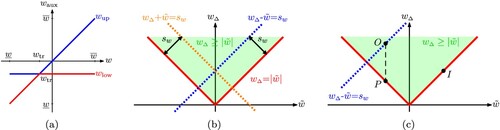
Before presenting the individual OPs, the basic principle for the space splitting of a decision variable is illustrated in this section providing graphical support. If collocation is used, the inputs as well as states represent decision variables. Thus, the input space and the state space can be split. The splitting procedure is presented using $w\in W[\underset{\_}{w},\overline{w}]$ as a representative decision variable which is split at the transition point $w=w_{\mathrm{t}\mathrm{r}}$. As illustrated in Figure 2(a), the auxiliary decision variables $w_{\mathrm{l}\mathrm{o}\mathrm{w}}\in W_{\mathrm{l}\mathrm{o}\mathrm{w}}[\underset{\_}{w},w_{\mathrm{t}\mathrm{r}}]$ and $w_{\mathrm{u}\mathrm{p}}\in W_{\mathrm{u}\mathrm{p}}[w_{\mathrm{t}\mathrm{r}},\overline{w}]$ are introduced aiming at satisfying the following relations: (8) $\begin{array}{r}{w}_{\mathrm{l}\mathrm{o}\mathrm{w}}=\left\{\begin{array}{ll}w& \mathrm{\forall }w\le w_{\mathrm{t}\mathrm{r}},\\ w_{\mathrm{t}\mathrm{r}}& \mathrm{e}\mathrm{l}\mathrm{s}\mathrm{e}\end{array}\right.,w_{\mathrm{u}\mathrm{p}}=\left\{\begin{array}{ll}w& \mathrm{\forall }w\ge w_{\mathrm{t}\mathrm{r}},\\ w_{\mathrm{t}\mathrm{r}}& \mathrm{e}\mathrm{l}\mathrm{s}\mathrm{e}\end{array}\right..\end{array}$(8)

Figure 1. Transformation of OP; Dotted and solid arrows represent approximated and exact transformations, respectively.

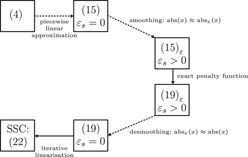
Figure 2. Space splitting. (a) Splitting of decision variable w into $w_{\mathrm{l}\mathrm{o}\mathrm{w}}$ and $w_{\mathrm{u}\mathrm{p}}$. (b) Absolute value constraint (9b(9b) $\begin{array}{rl}{g}_{\text{abs}}& =\underset{w_{\mathrm{\Delta }}}{\underbrace{w_{\text{up}}-w_{\text{low}}}}-|\underset{\tilde{w}}{\underbrace{w-w_{\text{tr}}}}|=0.\end{array}$(9b) ) and its relaxed linearisation according to (13a(13a) $\begin{array}{rl}& w_{-2\$\mathrm{\Delta }\$}-{\sigma }_w\tilde{w}=s_w\end{array}$(13a) ). (c) Projection after optimisation with initially wrong sign; I: initial guess; O: optimum; P: projection of optimum.

Lemma 2.1

The splitting relations (8(8) $\begin{array}{r}{w}_{\mathrm{l}\mathrm{o}\mathrm{w}}=\left\{\begin{array}{ll}w& \mathrm{\forall }w\le w_{\mathrm{t}\mathrm{r}},\\ w_{\mathrm{t}\mathrm{r}}& \mathrm{e}\mathrm{l}\mathrm{s}\mathrm{e}\end{array}\right.,w_{\mathrm{u}\mathrm{p}}=\left\{\begin{array}{ll}w& \mathrm{\forall }w\ge w_{\mathrm{t}\mathrm{r}},\\ w_{\mathrm{t}\mathrm{r}}& \mathrm{e}\mathrm{l}\mathrm{s}\mathrm{e}\end{array}\right..\end{array}$(8) ) can be implemented via the splitting constraints (9a) $\begin{array}{rl}{g}_{\text{aff}}& =w_{\text{up}}+w_{\text{low}}-(w+w_{\text{tr}})=0\end{array}$(9a) (9b) $\begin{array}{rl}{g}_{\text{abs}}& =\underset{w_{\mathrm{\Delta }}}{\underbrace{w_{\text{up}}-w_{\text{low}}}}-|\underset{\tilde{w}}{\underbrace{w-w_{\text{tr}}}}|=0.\end{array}$(9b)

Proof.

Solving (9a(9a) $\begin{array}{rl}{g}_{\text{aff}}& =w_{\text{up}}+w_{\text{low}}-(w+w_{\text{tr}})=0\end{array}$(9a) ) for one of the auxiliary decision variables yields (10a) $\begin{array}{r}{w}_{\mathrm{l}\mathrm{o}\mathrm{w}}=w+w_{\mathrm{t}\mathrm{r}}-w_{\mathrm{u}\mathrm{p}}.\end{array}$(10a) Inserting (10a(10a) $\begin{array}{r}{w}_{\mathrm{l}\mathrm{o}\mathrm{w}}=w+w_{\mathrm{t}\mathrm{r}}-w_{\mathrm{u}\mathrm{p}}.\end{array}$(10a) ) into (9b(9b) $\begin{array}{rl}{g}_{\text{abs}}& =\underset{w_{\mathrm{\Delta }}}{\underbrace{w_{\text{up}}-w_{\text{low}}}}-|\underset{\tilde{w}}{\underbrace{w-w_{\text{tr}}}}|=0.\end{array}$(9b) ) results in (10b) $\begin{array}{rl}{w}_{\mathrm{u}\mathrm{p}}& =\frac{1}{2}\left(|w-w_{\mathrm{t}\mathrm{r}}|+w+w_{\mathrm{t}\mathrm{r}}\right)\\ & \Rightarrow \left\{\begin{array}{ll}{w}_{\mathrm{u}\mathrm{p}}=w\stackrel{\left(10a\right)}{\Rightarrow }{w}_{\mathrm{l}\mathrm{o}\mathrm{w}}=w_{\mathrm{t}\mathrm{r}}& \mathrm{\forall }w\ge w_{\mathrm{t}\mathrm{r}}\\ w_{\mathrm{u}\mathrm{p}}=w_{\mathrm{t}\mathrm{r}}\stackrel{\left(10a\right)}{\Rightarrow }{w}_{\mathrm{l}\mathrm{o}\mathrm{w}}=w& \mathrm{\forall }w\le w_{\mathrm{t}\mathrm{r}}\end{array}\right..\end{array}$(10b) Thus, constraints (9) ensure the desired splitting according to (8(8) $\begin{array}{r}{w}_{\mathrm{l}\mathrm{o}\mathrm{w}}=\left\{\begin{array}{ll}w& \mathrm{\forall }w\le w_{\mathrm{t}\mathrm{r}},\\ w_{\mathrm{t}\mathrm{r}}& \mathrm{e}\mathrm{l}\mathrm{s}\mathrm{e}\end{array}\right.,w_{\mathrm{u}\mathrm{p}}=\left\{\begin{array}{ll}w& \mathrm{\forall }w\ge w_{\mathrm{t}\mathrm{r}},\\ w_{\mathrm{t}\mathrm{r}}& \mathrm{e}\mathrm{l}\mathrm{s}\mathrm{e}\end{array}\right..\end{array}$(8) ).

The AVC (9b(9b) $\begin{array}{rl}{g}_{\text{abs}}& =\underset{w_{\mathrm{\Delta }}}{\underbrace{w_{\text{up}}-w_{\text{low}}}}-|\underset{\tilde{w}}{\underbrace{w-w_{\text{tr}}}}|=0.\end{array}$(9b) ) is relaxed into a convex inequality constraint which can be depicted using two linear inequality constraints (11a) $\begin{array}{r}{g}_{\mathrm{a}\mathrm{b}\mathrm{s}}=w_{-2\$\mathrm{\Delta }\$}-|\tilde{w}|\ge 0\iff {\mathbf{\text{h}}}_{\mathrm{a}\mathrm{b}\mathrm{s}}=\left[\begin{array}{c}{w}_{-2\$\mathrm{\Delta }\$}-\tilde{w}\\ w_{-2\$\mathrm{\Delta }\$}+\tilde{w}\end{array}\right]\ge \mathbf{\text{0}}.\end{array}$(11a) Furthermore, the linearisation of the AVC based on the result of the preceding iteration $w_{\mathrm{p}\mathrm{r}\mathrm{e}\mathrm{v}}^{\star }$ is added as an additional objective term in form of an exact penalty function (11b) $\begin{array}{rl}{l}_{\mathrm{a}\mathrm{b}\mathrm{s}}& =w_{-2\$\mathrm{\Delta }\$}-{\sigma }_w\tilde{w}=0,{\sigma }_w\mathrm{s}\mathrm{i}\mathrm{g}\mathrm{n}\left({\tilde{w}}^{\star }\right)=\mathrm{s}\mathrm{i}\mathrm{g}\mathrm{n}(w_{\mathrm{p}\mathrm{r}\mathrm{e}\mathrm{v}}^{\star }-w_{\mathrm{t}\mathrm{r}})\end{array}$(11b) (11c) $\begin{array}{rl}& J_g\tau l_{\mathrm{a}\mathrm{b}\mathrm{s}}\end{array}$(11c)

with penalty parameter τ. Considering (11b(11b) $\begin{array}{rl}{l}_{\mathrm{a}\mathrm{b}\mathrm{s}}& =w_{-2\$\mathrm{\Delta }\$}-{\sigma }_w\tilde{w}=0,{\sigma }_w\mathrm{s}\mathrm{i}\mathrm{g}\mathrm{n}\left({\tilde{w}}^{\star }\right)=\mathrm{s}\mathrm{i}\mathrm{g}\mathrm{n}(w_{\mathrm{p}\mathrm{r}\mathrm{e}\mathrm{v}}^{\star }-w_{\mathrm{t}\mathrm{r}})\end{array}$(11b) ), the linearisation breaks down to choosing the sign ${\sigma }_w$ of the absolute value based on the previous solution $w_{\mathrm{p}\mathrm{r}\mathrm{e}\mathrm{v}}^{\star }$.Furthermore, the projection of the previous solution onto the constraints in (9) follows from (8(8) $\begin{array}{r}{w}_{\mathrm{l}\mathrm{o}\mathrm{w}}=\left\{\begin{array}{ll}w& \mathrm{\forall }w\le w_{\mathrm{t}\mathrm{r}},\\ w_{\mathrm{t}\mathrm{r}}& \mathrm{e}\mathrm{l}\mathrm{s}\mathrm{e}\end{array}\right.,w_{\mathrm{u}\mathrm{p}}=\left\{\begin{array}{ll}w& \mathrm{\forall }w\ge w_{\mathrm{t}\mathrm{r}},\\ w_{\mathrm{t}\mathrm{r}}& \mathrm{e}\mathrm{l}\mathrm{s}\mathrm{e}\end{array}\right..\end{array}$(8) ) and provides the initial solution, marked as $\breve{(\cdot )}$, for the subsequent iteration: (12) $\begin{array}{r}\breve{w}=w_{\mathrm{p}\mathrm{r}\mathrm{e}\mathrm{v}}^{\star },{\breve{w}}_{\mathrm{l}\mathrm{o}\mathrm{w}}=min(w_{\mathrm{p}\mathrm{r}\mathrm{e}\mathrm{v}}^{\star },w_{\mathrm{t}\mathrm{r}}),{\breve{w}}_{\mathrm{u}\mathrm{p}}=max(w_{\mathrm{p}\mathrm{r}\mathrm{e}\mathrm{v}}^{\star },w_{\mathrm{t}\mathrm{r}}).\end{array}$(12) The projection step is depicted in Figure 2(c) for an initial guess with a different sign than the computed solution: $\mathrm{s}\mathrm{i}\mathrm{g}\mathrm{n}\left({\breve{w}}_{\mathrm{p}\mathrm{r}\mathrm{e}\mathrm{v}}\right)\ne \mathrm{s}\mathrm{i}\mathrm{g}\mathrm{n}\left(w_{\mathrm{p}\mathrm{r}\mathrm{e}\mathrm{v}}^{\star }\right)$. For a graphical interpretation, the additional cost term (11c(11c) $\begin{array}{rl}& J_g\tau l_{\mathrm{a}\mathrm{b}\mathrm{s}}\end{array}$(11c) ) can be replaced by an additional relaxed equality constraint with the slack variable $s_w\ge 0$ being minimised via a penalty objective: (13a) $\begin{array}{rl}& w_{-2\$\mathrm{\Delta }\$}-{\sigma }_w\tilde{w}=s_w\end{array}$(13a) (13b) $\begin{array}{rl}& J_s\tau s_w.\end{array}$(13b) Since adding slack variables increases the number of decision variables, this is not desirable from an implementation standpoint; however, it fosters comprehension. The relaxation of constraint (13a(13a) $\begin{array}{rl}& w_{-2\$\mathrm{\Delta }\$}-{\sigma }_w\tilde{w}=s_w\end{array}$(13a) ) via the slack variable $s_w$ is necessary to avoid infeasibility, which is illustrated in Figure 2(b): Since $g_{\mathrm{a}\mathrm{b}\mathrm{s}}=w_{\mathrm{\Delta }}-|\tilde{w}|\ge 0$ holds, an unrelaxed constraint (13a(13a) $\begin{array}{rl}& w_{-2\$\mathrm{\Delta }\$}-{\sigma }_w\tilde{w}=s_w\end{array}$(13a) ) with $s_w\equiv 0$ would only allow values satisfying $\tilde{w}\le 0$ for ${\sigma }_w=-1$ and only values $\tilde{w}\ge 0$ for ${\sigma }_w=1$. However, the sign is based on the previous iteration and can thus be wrong. Then, a relaxation represented by the slack variable is necessary to allow values $\tilde{w}$ of the opposite region and avoid infeasibility. The sign is corrected for the subsequent iteration step to enable eradicating the additional objective (13b(13b) $\begin{array}{rl}& J_s\tau s_w.\end{array}$(13b) ) and thus the slack variable. This concludes that the initial solution does not have to represent a feasible solution, which results in robust initialisation behaviour. The relaxation via the slack variable $s_w$ in (13a(13a) $\begin{array}{rl}& w_{-2\$\mathrm{\Delta }\$}-{\sigma }_w\tilde{w}=s_w\end{array}$(13a) ) corresponds to the violation of constraint $l_{\mathrm{a}\mathrm{b}\mathrm{s}}$ via (11c(11c) $\begin{array}{rl}& J_g\tau l_{\mathrm{a}\mathrm{b}\mathrm{s}}\end{array}$(11c) ). The fact that the constraint violation will be large in case of a wrong sign is used as feedback for the algorithm. The algorithm will iterate until a feasible point satisfying $l_{\mathrm{a}\mathrm{b}\mathrm{s}}\approx 0\approx s_w$ is reached. Then, the additional objective (11c(11c) $\begin{array}{rl}& J_g\tau l_{\mathrm{a}\mathrm{b}\mathrm{s}}\end{array}$(11c) ) vanishes.

2.2.2. Piecewise linear approximation of optimisation problem

The first step towards a convex OP is the derivation of a piecewise linear approximation of the original problem (4). This is achieved by using the concept of space splitting presented in the previous section. Since multiple decision variables can be split, the formulation of the OP is posed using the augmented vector of decision variables (14) $\mathbf{\text{z}}={\left[\begin{array}{cccc}{\mathbf{\text{z}}}_0^{\mathrm{T}}& {\mathbf{\text{z}}}_{\frac{1}{2}}^{\mathrm{T}}& \dots & {\mathbf{\text{z}}}_{n_{\mathrm{s}\mathrm{e}\mathrm{g}}}^{\mathrm{T}}\end{array}\right]}^{\mathrm{T}},{\mathbf{\text{z}}}_k\left[\begin{array}{c}{\mathbf{\text{x}}}_k\\ {\mathbf{\text{u}}}_k\\ {\mathbf{\text{w}}}_{\mathrm{a}\mathrm{u}\mathrm{x},\mathrm{k}}\end{array}\right]\in {\mathbb{R}}^{n_z}$(14) with the auxiliary decision variables ${\mathbf{\text{w}}}_{\mathrm{a}\mathrm{u}\mathrm{x},\mathrm{k}}\in {\mathbb{R}}^{n_s}$. Therein some of the original states and inputs are excluded when they are depicted using affine transformations as illustrated in Section 2.3.1. The corresponding substitute problem is given for all $i\in I\text{and}k\in K$ by (15a) $\begin{array}{rl}\underset{\mathbf{\text{z}}}{min}& J\left(\mathbf{\text{w}}\right)\end{array}$(15a) (15b) $\begin{array}{rl}\mathrm{s}.\mathrm{t}.& {\widehat{\mathbf{\text{c}}}}_{\mathrm{c}\mathrm{o}\mathrm{l}\mathrm{l},i}\left(\mathbf{\text{z}}\right)={\mathbf{\text{c}}}_{\mathrm{c}\mathrm{o}\mathrm{l}\mathrm{l},i}(\mathbf{\text{w}}=\mathbf{\Phi }(\mathbf{\text{z}}),{\mathbf{\text{f}}}_{\mathrm{p}\mathrm{w}\mathrm{l}}={\mathbf{\Phi }}_{\mathrm{p}\mathrm{w}\mathrm{l}})=\mathbf{\text{0}},\end{array}$(15b) (15c) $\begin{array}{rl}& {\widehat{\mathbf{\text{c}}}}_k\left(\mathbf{\text{z}}\right)={\mathbf{\text{c}}}_k(\mathbf{\text{w}}=\mathbf{\Phi }(\mathbf{\text{z}}\left)\right)=\mathbf{\text{0}},\end{array}$(15c) (15d) $\begin{array}{rl}& {\widehat{\mathbf{\text{h}}}}_k\left(\mathbf{\text{z}}\right)={\mathbf{\text{h}}}_k(\mathbf{\text{w}}=\mathbf{\Phi }(\mathbf{\text{z}}\left)\right)\le \mathbf{\text{0}},\end{array}$(15d) (15e) $\begin{array}{rl}& {\widehat{\mathbf{\text{h}}}}_{\mathrm{z}\mathrm{c}\mathrm{s},k}\left(\mathbf{\text{z}}\right)\le \mathbf{\text{0}},\end{array}$(15e) (15f) $\begin{array}{rl}& {\mathbf{\text{g}}}_{\mathrm{a}\mathrm{f}\mathrm{f},k}\left(\mathbf{\text{z}}\right){\mathbf{\text{E}}}_{-2\$\mathrm{\Sigma }\$,k}{\mathbf{\text{w}}}_{\mathrm{a}\mathrm{u}\mathrm{x},k}-({\mathbf{\text{E}}}_{z,k}{\mathbf{\text{z}}}_k+{\mathbf{\text{w}}}_{\mathrm{t}\mathrm{r}})=\mathbf{\text{0}},\end{array}$(15f) (15g) $\begin{array}{rl}& {\mathbf{\text{g}}}_{\mathrm{a}\mathrm{b}\mathrm{s},k}\left(\mathbf{\text{z}}\right){\mathbf{\text{E}}}_{-2\$\mathrm{\Delta }\$,k}{\mathbf{\text{w}}}_{\mathrm{a}\mathrm{u}\mathrm{x},k}\\ & -\alpha (\underset{{\widetilde{\mathbf{\text{z}}}}_k}{\underbrace{{\mathbf{\text{E}}}_{z,k}{\mathbf{\text{z}}}_k-{\mathbf{\text{w}}}_{\mathrm{t}\mathrm{r}}}})=\mathbf{\text{0}}.\end{array}$(15g) Therein $\alpha (\cdot ):{\mathbb{R}}^{n_s}\to {\mathbb{R}}^{n_s}$ represents a function which applies the smoothable absolute value function (7(7) $\begin{array}{r}{\mathrm{a}\mathrm{b}\mathrm{s}}_{ϵ}\left(x\right)\sqrt{x^2+{ϵ}_s}\approx |x|=\mathrm{a}\mathrm{b}\mathrm{s}\left(x\right)\mathrm{w}\mathrm{i}\mathrm{t}\mathrm{h}0\le {ϵ}_s\ll 1\end{array}$(7) ) to each vector component individually: No smoothing occurs for ${ϵ}_s=0$. Furthermore, the right-hand side of the system equations (6(6) $\begin{array}{r}\mathbf{\text{f}}(\mathbf{\text{x}},\mathbf{\text{u}})=\left(\mathbf{\text{A}}\mathbf{\text{x}}+\mathbf{\text{B}}\mathbf{\text{u}}+\mathbf{\text{k}}\right)+{\mathbf{\text{f}}}_{\mathrm{p}\mathrm{w}\mathrm{l}}(\mathbf{\text{x}},\mathbf{\text{u}})\end{array}$(6) ) is depicted or approximated by the affine expression (16) $\begin{array}{r}\begin{array}{rl}{\mathbf{\text{f}}}_{\mathrm{\Phi }}(\mathbf{\text{x}},\mathbf{\text{u}},{\mathbf{\text{w}}}_{\mathrm{a}\mathrm{u}\mathrm{x}})=& \left(\mathbf{\text{A}}{\mathbf{\Phi }}_x(\mathbf{\text{x}},\mathbf{\text{u}},{\mathbf{\text{w}}}_{\mathrm{a}\mathrm{u}\mathrm{x}})+\mathbf{\text{B}}{\mathbf{\Phi }}_u(\mathbf{\text{x}},\mathbf{\text{u}},{\mathbf{\text{w}}}_{\mathrm{a}\mathrm{u}\mathrm{x}})+\mathbf{\text{k}}\right)+\\ & +{\mathbf{\Phi }}_{\mathrm{p}\mathrm{w}\mathrm{l}}(\mathbf{\text{x}},\mathbf{\text{u}},{\mathbf{\text{w}}}_{\mathrm{a}\mathrm{u}\mathrm{x}})\end{array}\end{array}$(16) with ${\mathbf{\Phi }}_u:{\mathbb{R}}^{n_z}\to {\mathbb{R}}^{n_u}$ and ${\mathbf{\Phi }}_x,{\mathbf{\Phi }}_{\mathrm{p}\mathrm{w}\mathrm{l}}:{\mathbb{R}}^{n_z}\to {\mathbb{R}}^{n_x}$ representing functions which are affine in the decision variables. Thus, (16(16) $\begin{array}{r}\begin{array}{rl}{\mathbf{\text{f}}}_{\mathrm{\Phi }}(\mathbf{\text{x}},\mathbf{\text{u}},{\mathbf{\text{w}}}_{\mathrm{a}\mathrm{u}\mathrm{x}})=& \left(\mathbf{\text{A}}{\mathbf{\Phi }}_x(\mathbf{\text{x}},\mathbf{\text{u}},{\mathbf{\text{w}}}_{\mathrm{a}\mathrm{u}\mathrm{x}})+\mathbf{\text{B}}{\mathbf{\Phi }}_u(\mathbf{\text{x}},\mathbf{\text{u}},{\mathbf{\text{w}}}_{\mathrm{a}\mathrm{u}\mathrm{x}})+\mathbf{\text{k}}\right)+\\ & +{\mathbf{\Phi }}_{\mathrm{p}\mathrm{w}\mathrm{l}}(\mathbf{\text{x}},\mathbf{\text{u}},{\mathbf{\text{w}}}_{\mathrm{a}\mathrm{u}\mathrm{x}})\end{array}\end{array}$(16) ) enables affine collocation constraints (15b(15b) $\begin{array}{rl}\mathrm{s}.\mathrm{t}.& {\widehat{\mathbf{\text{c}}}}_{\mathrm{c}\mathrm{o}\mathrm{l}\mathrm{l},i}\left(\mathbf{\text{z}}\right)={\mathbf{\text{c}}}_{\mathrm{c}\mathrm{o}\mathrm{l}\mathrm{l},i}(\mathbf{\text{w}}=\mathbf{\Phi }(\mathbf{\text{z}}),{\mathbf{\text{f}}}_{\mathrm{p}\mathrm{w}\mathrm{l}}={\mathbf{\Phi }}_{\mathrm{p}\mathrm{w}\mathrm{l}})=\mathbf{\text{0}},\end{array}$(15b) ). The transformation function $\mathbf{\Phi }\left(\mathbf{\text{z}}\right)$ in problem (15) represents the accumulation of the affine transformations ${\mathbf{\Phi }}_x$ and ${\mathbf{\Phi }}_u$ with $n_{\mathrm{\Phi }}=(n_x+n_u)n_{\mathrm{p}\mathrm{t}\mathrm{s}}$ yielding (17) $\begin{array}{rl}\mathbf{\text{w}}=\mathbf{\Phi }\left(\mathbf{\text{z}}\right)=\left[\begin{array}{c}{\mathbf{\Phi }}_0\\ ⋮\\ {\mathbf{\Phi }}_{n_{\mathrm{s}\mathrm{e}\mathrm{g}}}\end{array}\right]\widehat{\mathbf{\text{A}}}\mathbf{\text{z}}+\widehat{\mathbf{\text{b}}},{\mathbf{\Phi }}_k& \left[\begin{array}{c}{\mathbf{\Phi }}_x{\mid }_k\\ {\mathbf{\Phi }}_u{\mid }_k\end{array}\right]\end{array}$(17) with $\widehat{\mathbf{\text{A}}}\in {\mathbb{R}}^{n_{\mathrm{\Phi }}\times n_{\mathrm{\Phi }}}$ and $\widehat{\mathbf{\text{b}}}\in {\mathbb{R}}^{n_{\mathrm{\Phi }}}$ inserting the affine mapping (17(17) $\begin{array}{rl}\mathbf{\text{w}}=\mathbf{\Phi }\left(\mathbf{\text{z}}\right)=\left[\begin{array}{c}{\mathbf{\Phi }}_0\\ ⋮\\ {\mathbf{\Phi }}_{n_{\mathrm{s}\mathrm{e}\mathrm{g}}}\end{array}\right]\widehat{\mathbf{\text{A}}}\mathbf{\text{z}}+\widehat{\mathbf{\text{b}}},{\mathbf{\Phi }}_k& \left[\begin{array}{c}{\mathbf{\Phi }}_x{\mid }_k\\ {\mathbf{\Phi }}_u{\mid }_k\end{array}\right]\end{array}$(17) ) into the affine constraints (4c(4c) $\begin{array}{rl}& {\mathbf{\text{c}}}_k={\mathbf{\text{A}}}_c{\mathbf{\text{w}}}_k+{\mathbf{\text{k}}}_c=\mathbf{\text{0}}\mathrm{\forall }k\in K,\end{array}$(4c) ) and (4d(4d) $\begin{array}{rl}& {\mathbf{\text{h}}}_k\left({\mathbf{\text{w}}}_k\right)\le \mathbf{\text{0}}\mathrm{\forall }k\in K,\end{array}$(4d) ) results in the affine constraints (15c(15c) $\begin{array}{rl}& {\widehat{\mathbf{\text{c}}}}_k\left(\mathbf{\text{z}}\right)={\mathbf{\text{c}}}_k(\mathbf{\text{w}}=\mathbf{\Phi }(\mathbf{\text{z}}\left)\right)=\mathbf{\text{0}},\end{array}$(15c) ) and (15d(15d) $\begin{array}{rl}& {\widehat{\mathbf{\text{h}}}}_k\left(\mathbf{\text{z}}\right)={\mathbf{\text{h}}}_k(\mathbf{\text{w}}=\mathbf{\Phi }(\mathbf{\text{z}}\left)\right)\le \mathbf{\text{0}},\end{array}$(15d) ), respectively (Boyd & Vandenberghe, 2004, p. 79). Furthermore, the auxiliary variables are used to represent the ZCSs (4e(4e) $\begin{array}{rl}& {\mathbf{\text{h}}}_{\mathrm{z}\mathrm{c}\mathrm{s},k}\left({\mathbf{\text{w}}}_k\right)\le \mathbf{\text{0}}\mathrm{\forall }k\in K\end{array}$(4e) ) using convex functions ${\widehat{\mathbf{\text{h}}}}_{\mathrm{z}\mathrm{c}\mathrm{s}}$ in (15e(15e) $\begin{array}{rl}& {\widehat{\mathbf{\text{h}}}}_{\mathrm{z}\mathrm{c}\mathrm{s},k}\left(\mathbf{\text{z}}\right)\le \mathbf{\text{0}},\end{array}$(15e) ). In order to get a QP problem, these constraints are assumed to be affine or approximated by affine inequality constraints. The application of space splitting for the convexification of the original constraints will be shown in more detail in Section 2.3. The splitting constraints (15f(15f) $\begin{array}{rl}& {\mathbf{\text{g}}}_{\mathrm{a}\mathrm{f}\mathrm{f},k}\left(\mathbf{\text{z}}\right){\mathbf{\text{E}}}_{-2\$\mathrm{\Sigma }\$,k}{\mathbf{\text{w}}}_{\mathrm{a}\mathrm{u}\mathrm{x},k}-({\mathbf{\text{E}}}_{z,k}{\mathbf{\text{z}}}_k+{\mathbf{\text{w}}}_{\mathrm{t}\mathrm{r}})=\mathbf{\text{0}},\end{array}$(15f) ) and (15g(15g) $\begin{array}{rl}& {\mathbf{\text{g}}}_{\mathrm{a}\mathrm{b}\mathrm{s},k}\left(\mathbf{\text{z}}\right){\mathbf{\text{E}}}_{-2\$\mathrm{\Delta }\$,k}{\mathbf{\text{w}}}_{\mathrm{a}\mathrm{u}\mathrm{x},k}\\ & -\alpha (\underset{{\widetilde{\mathbf{\text{z}}}}_k}{\underbrace{{\mathbf{\text{E}}}_{z,k}{\mathbf{\text{z}}}_k-{\mathbf{\text{w}}}_{\mathrm{t}\mathrm{r}}}})=\mathbf{\text{0}}.\end{array}$(15g) ) represent the constraints (9a(9a) $\begin{array}{rl}{g}_{\text{aff}}& =w_{\text{up}}+w_{\text{low}}-(w+w_{\text{tr}})=0\end{array}$(9a) ) and (9b(9b) $\begin{array}{rl}{g}_{\text{abs}}& =\underset{w_{\mathrm{\Delta }}}{\underbrace{w_{\text{up}}-w_{\text{low}}}}-|\underset{\tilde{w}}{\underbrace{w-w_{\text{tr}}}}|=0.\end{array}$(9b) ), respectively. These constraints are necessary to ensure that problem (15) correctly represents the original problem (4). They implement a bisection of selected decision variables at predefined transition values which are stored in the vector ${\mathbf{\text{w}}}_{\mathrm{t}\mathrm{r}}$. The matrices ${\mathbf{\text{E}}}_{\mathrm{\Sigma },k}$, ${\mathbf{\text{E}}}_{\mathrm{\Delta },k}$ and ${\mathbf{\text{E}}}_{z,k}$ are selection matrices extracting the desired decision variables. It is assumed that $\frac{n_s}{2}$ decision variables are split at each collocation point.

Depending on the individual approximations of the nonlinear constraints, the piecewise linear representation is subject to some error. The approximation error of this substitute problem is defined beforehand by the implemented number of space subdivisions. If the original problem is piecewise linear, this substitute problem can be an exact representation.

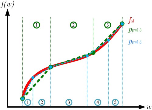
Remark 2.1

Let $f_{\mathrm{n}\mathrm{l}}\left(w\right)$ represent a nonlinearity within a constraint depending on the decision variable representative w, as depicted in Figure 3. Then, the total absolute error of the piecewise linear approximation $p_{\mathrm{p}\mathrm{w}\mathrm{l}}\left(w\right)$ is given by the sum of absolute errors at each collocation point of the decision variable: (18) $\begin{array}{r}{e}_{\mathrm{p}\mathrm{w}\mathrm{l}}=\sum _{k\in K}|f_{\mathrm{n}\mathrm{l}}\left(w_k\right)-p_{\mathrm{p}\mathrm{w}\mathrm{l}}\left(w_k\right)|.\end{array}$(18) An adequate number and position of knot points for the segmentation into piecewise linear parts achieve sufficiently small approximation errors. However, a higher number of splitting segments increases the size of the OP influencing the computation time.

Figure 3. Approximation of nonlinearity $f_{\mathrm{n}\mathrm{l}}$ with three-/five-segmented piecewise linear polynom $p_{\mathrm{p}\mathrm{w}\mathrm{l},3}/p_{\mathrm{p}\mathrm{w}\mathrm{l},5}$; Approximation error can be reduced with an increasing number of splitting segments.

2.2.3. Nonconvex optimisation problem with convex feasible set

The absolute values in equality constraint (15g(15g) $\begin{array}{rl}& {\mathbf{\text{g}}}_{\mathrm{a}\mathrm{b}\mathrm{s},k}\left(\mathbf{\text{z}}\right){\mathbf{\text{E}}}_{-2\$\mathrm{\Delta }\$,k}{\mathbf{\text{w}}}_{\mathrm{a}\mathrm{u}\mathrm{x},k}\\ & -\alpha (\underset{{\widetilde{\mathbf{\text{z}}}}_k}{\underbrace{{\mathbf{\text{E}}}_{z,k}{\mathbf{\text{z}}}_k-{\mathbf{\text{w}}}_{\mathrm{t}\mathrm{r}}}})=\mathbf{\text{0}}.\end{array}$(15g) ) still prohibit convexity. Deploying the theory of exact penalty functions (Di Pillo & Grippo, 1989; Han & Mangasarian, 1979), the absolute value equality constraints are moved to the objective without compromising optimality:

Theorem 2.1

Let $\overline{\mathbf{\text{z}}}$ be a stationary point of the OP (19a) $\begin{array}{rl}\underset{\mathbf{\text{z}}}{min}& J\left(\mathbf{\text{w}}\right)+\tau \sum _{k\in K}\underset{={∥{\mathbf{\text{g}}}_{\text{abs},k}∥}_1}{\underbrace{\sum _{j=1}^{n_s}{g}_{\text{abs},k,j}}}\end{array}$(19a) (19b) $\begin{array}{rl}\mathrm{s}.\mathrm{t}.& \left[\begin{array}{ccc}{\widehat{\mathbf{\text{c}}}}_{\text{coll},i}^{\mathrm{T}}& {\widehat{\mathbf{\text{c}}}}_k^{\mathrm{T}}& {\mathbf{\text{g}}}_{\text{aff},k}^{\mathrm{T}}\end{array}\right]={\mathbf{\text{0}}}^{\mathrm{T}}\mathrm{\forall }i\in I,k\in K\end{array}$(19b) (19c) $\begin{array}{rl}& \left[\begin{array}{cc}{\widehat{\mathbf{\text{h}}}}_k^{\mathrm{T}}& {\widehat{\mathbf{\text{h}}}}_{\text{zcs},k}^{\mathrm{T}}\end{array}\right]\le {\mathbf{\text{0}}}^{\mathrm{T}}\mathrm{\forall }k\in K\end{array}$(19c) (19d) $\begin{array}{rl}& {\mathbf{\text{g}}}_{\text{abs},k}\ge \mathbf{\text{0}}\mathrm{\forall }k\in K\end{array}$(19d) with $\mathit{\lambda }$ representing the Lagrangian multipliers of the corresponding equality constraints. Since a $L_1-\mathrm{n}\mathrm{o}\mathrm{r}\mathrm{m}$ is an exact penalty function, $\overline{\mathbf{\text{z}}}$ is a critical point of problem (15) for ${ϵ}_s>0$ and sufficiently large but finite penalty weights $\tau \ge {∥\mathit{\lambda }∥}_{\mathrm{\infty }}$.

Proof.

The prerequisite for the optima recovery is that the optimality conditions are admissible for problem (15) (Nocedal & Wright, 2006, p. 507). For this purpose, the linear independence constraint qualification (LICQ) (Nocedal & Wright, 2006, p. 320) is analysed subsequently. Since the transformation $\mathbf{\Phi }\left(\mathbf{\text{z}}\right)$ in (17(17) $\begin{array}{rl}\mathbf{\text{w}}=\mathbf{\Phi }\left(\mathbf{\text{z}}\right)=\left[\begin{array}{c}{\mathbf{\Phi }}_0\\ ⋮\\ {\mathbf{\Phi }}_{n_{\mathrm{s}\mathrm{e}\mathrm{g}}}\end{array}\right]\widehat{\mathbf{\text{A}}}\mathbf{\text{z}}+\widehat{\mathbf{\text{b}}},{\mathbf{\Phi }}_k& \left[\begin{array}{c}{\mathbf{\Phi }}_x{\mid }_k\\ {\mathbf{\Phi }}_u{\mid }_k\end{array}\right]\end{array}$(17) ) is affine, the gradients of the transformed basic constraints (15c(15c) $\begin{array}{rl}& {\widehat{\mathbf{\text{c}}}}_k\left(\mathbf{\text{z}}\right)={\mathbf{\text{c}}}_k(\mathbf{\text{w}}=\mathbf{\Phi }(\mathbf{\text{z}}\left)\right)=\mathbf{\text{0}},\end{array}$(15c) ) and (15d(15d) $\begin{array}{rl}& {\widehat{\mathbf{\text{h}}}}_k\left(\mathbf{\text{z}}\right)={\mathbf{\text{h}}}_k(\mathbf{\text{w}}=\mathbf{\Phi }(\mathbf{\text{z}}\left)\right)\le \mathbf{\text{0}},\end{array}$(15d) ) remain linearly independent if the original constraints $\mathbf{\text{c}}\left(\mathbf{\text{w}}\right):{\mathbb{R}}^{n_w}\to {\mathbb{R}}^{n_c}$ and $\mathbf{\text{h}}\left(\mathbf{\text{w}}\right):{\mathbb{R}}^{n_w}\to {\mathbb{R}}^{n_h}$ are linearly independent. This can be verified for $i\in \{1,\dots ,n_c\}$ and $j\in \{1,\dots ,n_h\}$ via (20a) $\begin{array}{r}{\mathrm{\nabla }}_{\mathbf{\text{z}}}{\hat{c}}_i\left(\mathbf{\text{z}}\right)={\left(\frac{\mathrm{\partial }{c}_i\left(\mathbf{\Phi }\right(\mathbf{\text{z}}\left)\right)}{\mathrm{\partial }\mathbf{\Phi }}\frac{\mathrm{\partial }\mathbf{\Phi }}{\mathrm{\partial }\mathbf{\text{z}}}\right)}^{\mathrm{T}}={\widehat{\mathbf{\text{A}}}}^{\mathrm{T}}{\mathrm{\nabla }}_{\mathbf{\text{w}}}{c}_i(\mathbf{\text{w}}=\mathbf{\Phi }(\mathbf{\text{z}}\left)\right)\end{array}$(20a) (20b) $\begin{array}{r}{\mathrm{\nabla }}_{\mathbf{\text{z}}}\widehat{h_j}\left(\mathbf{\text{z}}\right)={\left(\frac{\mathrm{\partial }{h}_j\left(\mathbf{\Phi }\right(\mathbf{\text{z}}\left)\right)}{\mathrm{\partial }\mathbf{\Phi }}\frac{\mathrm{\partial }\mathbf{\Phi }}{\mathrm{\partial }\mathbf{\text{z}}}\right)}^{\mathrm{T}}={\widehat{\mathbf{\text{A}}}}^{\mathrm{T}}{\mathrm{\nabla }}_{\mathbf{\text{w}}}{h}_j(\mathbf{\text{w}}=\mathbf{\Phi }(\mathbf{\text{z}}\left)\right).\end{array}$(20b) The gradients of the splitting constraints (15f(15f) $\begin{array}{rl}& {\mathbf{\text{g}}}_{\mathrm{a}\mathrm{f}\mathrm{f},k}\left(\mathbf{\text{z}}\right){\mathbf{\text{E}}}_{-2\$\mathrm{\Sigma }\$,k}{\mathbf{\text{w}}}_{\mathrm{a}\mathrm{u}\mathrm{x},k}-({\mathbf{\text{E}}}_{z,k}{\mathbf{\text{z}}}_k+{\mathbf{\text{w}}}_{\mathrm{t}\mathrm{r}})=\mathbf{\text{0}},\end{array}$(15f) ) and (15g(15g) $\begin{array}{rl}& {\mathbf{\text{g}}}_{\mathrm{a}\mathrm{b}\mathrm{s},k}\left(\mathbf{\text{z}}\right){\mathbf{\text{E}}}_{-2\$\mathrm{\Delta }\$,k}{\mathbf{\text{w}}}_{\mathrm{a}\mathrm{u}\mathrm{x},k}\\ & -\alpha (\underset{{\widetilde{\mathbf{\text{z}}}}_k}{\underbrace{{\mathbf{\text{E}}}_{z,k}{\mathbf{\text{z}}}_k-{\mathbf{\text{w}}}_{\mathrm{t}\mathrm{r}}}})=\mathbf{\text{0}}.\end{array}$(15g) ) are by definition linearly independent from each other and from the remaining constraints. Furthermore, it can be assumed without loss of generality that the gradients of the collocation constraints (15b(15b) $\begin{array}{rl}\mathrm{s}.\mathrm{t}.& {\widehat{\mathbf{\text{c}}}}_{\mathrm{c}\mathrm{o}\mathrm{l}\mathrm{l},i}\left(\mathbf{\text{z}}\right)={\mathbf{\text{c}}}_{\mathrm{c}\mathrm{o}\mathrm{l}\mathrm{l},i}(\mathbf{\text{w}}=\mathbf{\Phi }(\mathbf{\text{z}}),{\mathbf{\text{f}}}_{\mathrm{p}\mathrm{w}\mathrm{l}}={\mathbf{\Phi }}_{\mathrm{p}\mathrm{w}\mathrm{l}})=\mathbf{\text{0}},\end{array}$(15b) ), of the basic constraints (15c(15c) $\begin{array}{rl}& {\widehat{\mathbf{\text{c}}}}_k\left(\mathbf{\text{z}}\right)={\mathbf{\text{c}}}_k(\mathbf{\text{w}}=\mathbf{\Phi }(\mathbf{\text{z}}\left)\right)=\mathbf{\text{0}},\end{array}$(15c) )–(15d(15d) $\begin{array}{rl}& {\widehat{\mathbf{\text{h}}}}_k\left(\mathbf{\text{z}}\right)={\mathbf{\text{h}}}_k(\mathbf{\text{w}}=\mathbf{\Phi }(\mathbf{\text{z}}\left)\right)\le \mathbf{\text{0}},\end{array}$(15d) ) and of the ZCS-constraints (15e(15e) $\begin{array}{rl}& {\widehat{\mathbf{\text{h}}}}_{\mathrm{z}\mathrm{c}\mathrm{s},k}\left(\mathbf{\text{z}}\right)\le \mathbf{\text{0}},\end{array}$(15e) ) are linearly independent. Thus, if the LICQ holds for the original problem (4), then it is also satisfied by the problem (15). By choosing a sufficiently small but positive smoothing parameter $0<{ϵ}_s\ll 1$, the prerequisite of continuous differentiable objective and constraint functions is given while approximation errors are kept small. Thus, the optimal solution will satisfy the Karush–Kuhn–Tucker conditions (Nocedal & Wright, 2006, p. 321).

Constraints (19d(19d) $\begin{array}{rl}& {\mathbf{\text{g}}}_{\text{abs},k}\ge \mathbf{\text{0}}\mathrm{\forall }k\in K\end{array}$(19d) ) are added to enable omitting the norm in the objective as illustrated in (19a(19a) $\begin{array}{rl}\underset{\mathbf{\text{z}}}{min}& J\left(\mathbf{\text{w}}\right)+\tau \sum _{k\in K}\underset{={∥{\mathbf{\text{g}}}_{\text{abs},k}∥}_1}{\underbrace{\sum _{j=1}^{n_s}{g}_{\text{abs},k,j}}}\end{array}$(19a) ). Since ${\mathbf{\text{g}}}_{\mathrm{a}\mathrm{b}\mathrm{s},k}$ is a vector of concave functions, the AVCs (19d(19d) $\begin{array}{rl}& {\mathbf{\text{g}}}_{\text{abs},k}\ge \mathbf{\text{0}}\mathrm{\forall }k\in K\end{array}$(19d) ) represent a convex set. Thus, the feasible set of OP (19) is convex.

2.2.4. Convex optimisation problem for iterative solution

From Theorem 2.1 follows that solving (19) provides the solution for problem (15) assuming ${ϵ}_s>0$. Unfortunately, the augmented objective (19a(19a) $\begin{array}{rl}\underset{\mathbf{\text{z}}}{min}& J\left(\mathbf{\text{w}}\right)+\tau \sum _{k\in K}\underset{={∥{\mathbf{\text{g}}}_{\text{abs},k}∥}_1}{\underbrace{\sum _{j=1}^{n_s}{g}_{\text{abs},k,j}}}\end{array}$(19a) ) is nonconvex, which will be addressed via linearisation. Subsequently, the smoothing is removed by setting ${ϵ}_s=0$ since it will not be required for continuous differentiability. Omitting the smoothing represents an approximation to the smoothed version of (19); however, it is beneficial from a practical standpoint since the splitting constraints are exact for ${ϵ}_s=0$. Furthermore, it enables representing the AVCs (19d(19d) $\begin{array}{rl}& {\mathbf{\text{g}}}_{\text{abs},k}\ge \mathbf{\text{0}}\mathrm{\forall }k\in K\end{array}$(19d) ) by two affine inequalities which yields exclusively affine constraints required for an LP and QP problem. For a convex OP, the absolute value of the AVCs in the augmented objective is linearised around the points ${\widetilde{\mathbf{\text{z}}}}_k^{\star }\in {\mathbb{R}}^{n_s}$ yielding the linearised constraints (21a) $\begin{array}{r}{\mathbf{\text{l}}}_{\mathrm{a}\mathrm{b}\mathrm{s},k}(\mathbf{\text{z}},{\widetilde{\mathbf{\text{z}}}}_k^{\star }){\mathbf{\text{E}}}_{-2\$\mathrm{\Delta }\$,k}{\mathbf{\text{w}}}_{\mathrm{a}\mathrm{u}\mathrm{x},k}-{\mathbf{\Sigma }}_k{\widetilde{\mathbf{\text{z}}}}_k=\mathbf{\text{0}}\mathrm{\forall }k\in K,\end{array}$(21a) which represent (11b(11b) $\begin{array}{rl}{l}_{\mathrm{a}\mathrm{b}\mathrm{s}}& =w_{-2\$\mathrm{\Delta }\$}-{\sigma }_w\tilde{w}=0,{\sigma }_w\mathrm{s}\mathrm{i}\mathrm{g}\mathrm{n}\left({\tilde{w}}^{\star }\right)=\mathrm{s}\mathrm{i}\mathrm{g}\mathrm{n}(w_{\mathrm{p}\mathrm{r}\mathrm{e}\mathrm{v}}^{\star }-w_{\mathrm{t}\mathrm{r}})\end{array}$(11b) ), with the linearisation points being stored in matrix (21b) $\begin{array}{r}\begin{array}{rl}\mathbf{\Sigma }& \left[\begin{array}{cccc}{\mathbf{\Sigma }}_0& {\mathbf{\Sigma }}_{\frac{1}{2}}& \dots & {\mathbf{\Sigma }}_{n_{\mathrm{s}\mathrm{e}\mathrm{g}}}\end{array}\right]\mathrm{w}\mathrm{i}\mathrm{t}\mathrm{h}\\ {\mathbf{\Sigma }}_k& \mathrm{d}\mathrm{i}\mathrm{a}\mathrm{g}\left(\mathrm{s}\mathrm{i}\mathrm{g}\mathrm{n}\left({\tilde{z}}_{k,1}^{\star }\right),\dots ,\mathrm{s}\mathrm{i}\mathrm{g}\mathrm{n}\left({\tilde{z}}_{k,n_s}^{\star }\right)\right).\end{array}\end{array}$(21b) Comparing (15g(15g) $\begin{array}{rl}& {\mathbf{\text{g}}}_{\mathrm{a}\mathrm{b}\mathrm{s},k}\left(\mathbf{\text{z}}\right){\mathbf{\text{E}}}_{-2\$\mathrm{\Delta }\$,k}{\mathbf{\text{w}}}_{\mathrm{a}\mathrm{u}\mathrm{x},k}\\ & -\alpha (\underset{{\widetilde{\mathbf{\text{z}}}}_k}{\underbrace{{\mathbf{\text{E}}}_{z,k}{\mathbf{\text{z}}}_k-{\mathbf{\text{w}}}_{\mathrm{t}\mathrm{r}}}})=\mathbf{\text{0}}.\end{array}$(15g) ) and (21a(21a) $\begin{array}{r}{\mathbf{\text{l}}}_{\mathrm{a}\mathrm{b}\mathrm{s},k}(\mathbf{\text{z}},{\widetilde{\mathbf{\text{z}}}}_k^{\star }){\mathbf{\text{E}}}_{-2\$\mathrm{\Delta }\$,k}{\mathbf{\text{w}}}_{\mathrm{a}\mathrm{u}\mathrm{x},k}-{\mathbf{\Sigma }}_k{\widetilde{\mathbf{\text{z}}}}_k=\mathbf{\text{0}}\mathrm{\forall }k\in K,\end{array}$(21a) ) shows that the linearisation breaks down to a binary decision: choosing the correct sign of the absolute value term ${\widetilde{\mathbf{\text{z}}}}_k$. The linearisation (21a(21a) $\begin{array}{r}{\mathbf{\text{l}}}_{\mathrm{a}\mathrm{b}\mathrm{s},k}(\mathbf{\text{z}},{\widetilde{\mathbf{\text{z}}}}_k^{\star }){\mathbf{\text{E}}}_{-2\$\mathrm{\Delta }\$,k}{\mathbf{\text{w}}}_{\mathrm{a}\mathrm{u}\mathrm{x},k}-{\mathbf{\Sigma }}_k{\widetilde{\mathbf{\text{z}}}}_k=\mathbf{\text{0}}\mathrm{\forall }k\in K,\end{array}$(21a) ) is affine in the decision variables. Since the sum of convex functions preserves convexity (Boyd & Vandenberghe, 2004, p. 79), the composite objective function is then convex in the decision variables. With all constraints being affine, using linearisation (21a(21a) $\begin{array}{r}{\mathbf{\text{l}}}_{\mathrm{a}\mathrm{b}\mathrm{s},k}(\mathbf{\text{z}},{\widetilde{\mathbf{\text{z}}}}_k^{\star }){\mathbf{\text{E}}}_{-2\$\mathrm{\Delta }\$,k}{\mathbf{\text{w}}}_{\mathrm{a}\mathrm{u}\mathrm{x},k}-{\mathbf{\Sigma }}_k{\widetilde{\mathbf{\text{z}}}}_k=\mathbf{\text{0}}\mathrm{\forall }k\in K,\end{array}$(21a) ) results in the convex QP problem (22a) $\begin{array}{rl}\underset{\mathbf{\text{z}}}{min}& J_{\mathrm{t}\mathrm{o}\mathrm{t}}(\mathbf{\text{z}},{\mathbf{\text{z}}}^{\star })J\left(\mathbf{\text{w}}\right)+\tau \sum _{k\in K}\sum _{j=1}^{n_s}{l}_{\mathrm{a}\mathrm{b}\mathrm{s},k,j}\end{array}$(22a) (22b) $\begin{array}{rl}\mathrm{s}.\mathrm{t}.& {\widehat{\mathbf{\text{c}}}}_{\mathrm{c}\mathrm{o}\mathrm{l}\mathrm{l},i}=\mathbf{\text{0}}\mathrm{\forall }i\in I,\end{array}$(22b) (22c) $\begin{array}{rl}& {\mathbf{\text{c}}}_{\mathrm{t}\mathrm{o}\mathrm{t},k}^{\mathrm{T}}\left(\mathbf{\text{z}}\right)\left[\begin{array}{cc}{\widehat{\mathbf{\text{c}}}}_k^{\mathrm{T}}& {\mathbf{\text{g}}}_{\mathrm{a}\mathrm{f}\mathrm{f},k}^{\mathrm{T}}\end{array}\right]={\mathbf{\text{0}}}^{\mathrm{T}}\mathrm{\forall }k\in K,\end{array}$(22c) (22d) $\begin{array}{rl}& {\mathbf{\text{h}}}_{\mathrm{t}\mathrm{o}\mathrm{t},k}^{\mathrm{T}}\left(\mathbf{\text{z}}\right)\left[\begin{array}{cc}{\widehat{\mathbf{\text{h}}}}_k^{\mathrm{T}}& {\widehat{\mathbf{\text{h}}}}_{\mathrm{z}\mathrm{c}\mathrm{s},k}^{\mathrm{T}}\end{array}\right]\le {\mathbf{\text{0}}}^{\mathrm{T}}\mathrm{\forall }k\in K,\end{array}$(22d) (22e) $\begin{array}{rl}& {\mathbf{\text{h}}}_{\mathrm{a}\mathrm{b}\mathrm{s},k}\left(\mathbf{\text{z}}\right)\left[\begin{array}{c}{\mathbf{\text{E}}}_{-2\$\mathrm{\Delta }\$,k}{\mathbf{\text{w}}}_{\mathrm{a}\mathrm{u}\mathrm{x},k}-{\widetilde{\mathbf{\text{z}}}}_k\\ {\mathbf{\text{E}}}_{-2\$\mathrm{\Delta }\$,k}{\mathbf{\text{w}}}_{\mathrm{a}\mathrm{u}\mathrm{x},k}+{\widetilde{\mathbf{\text{z}}}}_k\end{array}\right]\ge \mathbf{\text{0}}\mathrm{\forall }k\in K.\end{array}$(22e) For linear objectives $J\left(\mathbf{\text{w}}\right)$, the SSC approach results in a LP problem. The convex problem (22) is iteratively solved, whereas the linearisation points in $\mathbf{\Sigma }$ are updated based on the solution ${\mathbf{\text{z}}}^{{\star }^{\mathrm{T}}}=\left[\begin{array}{ccc}{\mathbf{\text{z}}}_0^{{\star }^{\mathrm{T}}}& \dots & {\mathbf{\text{z}}}_{n_{\mathrm{s}\mathrm{e}\mathrm{g}}}^{{\star }^{\mathrm{T}}}\end{array}\right]$ of the preceding iteration yielding (23) $\begin{array}{r}{\widetilde{\mathbf{\text{z}}}}_k^{\star }={\mathbf{\text{E}}}_{z,k}{\mathbf{\text{z}}}_k^{\star }-{\mathbf{\text{w}}}_{\mathrm{t}\mathrm{r}}\mathrm{\forall }k\in K.\end{array}$(23) However, the question arises if replacing the constraint ${\mathbf{\text{g}}}_{\mathrm{a}\mathrm{b}\mathrm{s}}$ in the objective with its linearisation ${\mathbf{\text{l}}}_{\mathrm{a}\mathrm{b}\mathrm{s}}$ falsifies the solution. This motivates the following lemma:

Lemma 2.2

The satisfaction of ${\mathbf{\text{h}}}_{abs,k}\left(\mathbf{\text{z}}\right)\ge \mathbf{0}$ and ${\mathbf{\text{l}}}_{abs,k}(\mathbf{\text{z}},{\widetilde{\mathbf{\text{z}}}}_k^{\star })=\mathbf{0}$ concludes ${\mathbf{\text{g}}}_{abs,k}\left(\mathbf{\text{z}}\right)=\mathbf{0}$, independently of the linearisation point ${\widetilde{\mathbf{\text{z}}}}_k^{\star }$.

Proof.

This can be verified using Figure 2(b) as graphical support. For this purpose, the following equations are given in general notation and are compared with the equations from the illustrative example in Section 2.2.1 using the vector of decision variables ${\mathbf{\text{z}}}_{\mathrm{e}\mathrm{x}}={\left[\begin{array}{ccc}w& w_{\mathrm{u}\mathrm{p}}& w_{\mathrm{l}\mathrm{o}\mathrm{w}}\end{array}\right]}^{\mathrm{T}}$. The nonsmoothed absolute value constraint $g_{\mathrm{a}\mathrm{b}\mathrm{s},k,j}$ spans the following set of points: (24a) $\begin{array}{r}\begin{array}{rl}{G}_{k,j}\left(\mathbf{\text{z}}\right)& \{\mathbf{\text{z}}|{\mathbf{\text{e}}}_{-2\$\mathrm{\Delta }\$,k}^{\mathrm{T}}{\mathbf{\text{w}}}_{\mathrm{a}\mathrm{u}\mathrm{x},k}-|{\tilde{z}}_{k,j}|=0\}\\ & \widehat{=}\{{\mathbf{\text{z}}}_{\mathrm{e}\mathrm{x}}|w_{-2\$\mathrm{\Delta }\$}-|\tilde{w}|=0\}\end{array}\end{array}$(24a) with ${\mathbf{\text{e}}}_{\mathrm{\Delta },k}^{\mathrm{T}}$ representing the jth row of matrix ${\mathbf{\text{E}}}_{\mathrm{\Delta },k}$. The admissible points for the AVC-linearisation $l_{\mathrm{a}\mathrm{b}\mathrm{s},k,j}$ are given by (24b) $\begin{array}{r}\begin{array}{rl}{L}_{k,j}(\mathbf{\text{z}},{\tilde{z}}_{k,j}^{\star })& \{\mathbf{\text{z}}|{\mathbf{\text{e}}}_{-2\$\mathrm{\Delta }\$,k}^{\mathrm{T}}{\mathbf{\text{w}}}_{\mathrm{a}\mathrm{u}\mathrm{x},k}-\mathrm{s}\mathrm{i}\mathrm{g}\mathrm{n}({\tilde{z}}_{k,j}^{\star }){\tilde{z}}_{k,j}=0\}\\ & \widehat{=}\{{\mathbf{\text{z}}}_{\mathrm{e}\mathrm{x}}|w_{-2\$\mathrm{\Delta }\$}-{\sigma }_w\tilde{w}=0\}\end{array}\end{array}$(24b) representing the infinite extension of the positive and negative branch of the AVC for ${\tilde{z}}_{k,j}^{\star },{\sigma }_w\ge 0$ and ${\tilde{z}}_{k,j}^{\star },{\sigma }_w\le 0$, respectively. Then, the intersection with the admissible points of the inequality constraint ${\mathbf{\text{h}}}_{\mathrm{a}\mathrm{b}\mathrm{s},k,j}$ (24c) $\begin{array}{r}\begin{array}{rl}{H}_{k,j}\left(\mathbf{\text{z}}\right)& \left\{\mathbf{\text{z}}|\left[\begin{array}{c}{\mathbf{\text{e}}}_{-2\$\mathrm{\Delta }\$,k}^{\mathrm{T}}{\mathbf{\text{w}}}_{\mathrm{a}\mathrm{u}\mathrm{x},k}-{\tilde{z}}_{k,j}\\ {\mathbf{\text{e}}}_{-2\$\mathrm{\Delta }\$,k}^{\mathrm{T}}{\mathbf{\text{w}}}_{\mathrm{a}\mathrm{u}\mathrm{x},k}+{\tilde{z}}_{k,j}\end{array}\right]\ge \mathbf{\text{0}}\right\}\\ & \widehat{=}\left\{{\mathbf{\text{z}}}_{\mathrm{e}\mathrm{x}}|\left[\begin{array}{c}{w}_{-2\$\mathrm{\Delta }\$}-\tilde{w}\\ w_{-2\$\mathrm{\Delta }\$}+\tilde{w}\end{array}\right]\ge \mathbf{\text{0}}\right\}\end{array}\end{array}$(24c) provides the sets (24d) $\begin{array}{rl}{N}_{k,j}\left(\mathbf{\text{z}}\right)& \{\mathbf{\text{z}}|\mathbf{\text{z}}\in H_{k,j},\mathbf{\text{z}}\in L_{k,j}(\mathbf{\text{z}},{\tilde{z}}_{k,j}^{\star }\left){|}_{{\tilde{z}}_{k,j}^{\star }\le 0}\right\}\end{array}$(24d) (24e) $\begin{array}{rl}{P}_{k,j}\left(\mathbf{\text{z}}\right)& \{\mathbf{\text{z}}|\mathbf{\text{z}}\in H_{k,j},\mathbf{\text{z}}\in L_{k,j}(\mathbf{\text{z}},{\tilde{z}}_{k,j}^{\star }\left){|}_{{\tilde{z}}_{k,j}^{\star }\ge 0}\right\},\end{array}$(24e) which represent the negative and positive branch of the AVC and are thus a subset: $N_{k,j},P_{k,j}\subset G_{k,j}$.

This important lemma ensures that convergence of problem (22) to a solution which satisfies the linearised constraints ${\mathbf{\text{l}}}_{abs,k}(\mathbf{\text{z}},{\widetilde{\mathbf{\text{z}}}}_k^{\star })=\mathbf{\text{0}}$ also fulfils the original nonlinear constraints ${\mathbf{\text{g}}}_{abs,k}\left(\mathbf{\text{z}}\right)=\mathbf{\text{0}}$ in (15g(15g) $\begin{array}{rl}& {\mathbf{\text{g}}}_{\mathrm{a}\mathrm{b}\mathrm{s},k}\left(\mathbf{\text{z}}\right){\mathbf{\text{E}}}_{-2\$\mathrm{\Delta }\$,k}{\mathbf{\text{w}}}_{\mathrm{a}\mathrm{u}\mathrm{x},k}\\ & -\alpha (\underset{{\widetilde{\mathbf{\text{z}}}}_k}{\underbrace{{\mathbf{\text{E}}}_{z,k}{\mathbf{\text{z}}}_k-{\mathbf{\text{w}}}_{\mathrm{t}\mathrm{r}}}})=\mathbf{\text{0}}.\end{array}$(15g) ).

2.2.5. Space splitting convexification algorithm

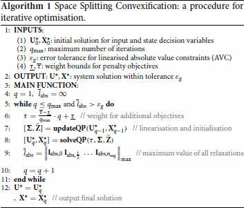
Subsequently, the SSC algorithm 1 is presented in detail and the proof of its convergence is provided. The algorithm inputs are described in line 1. An initial solution for the inputs ${\mathbf{\text{U}}}_0^{\star }\in {\mathbb{R}}^{n_u\times n_{\mathrm{p}\mathrm{t}\mathrm{s}}}$ and states ${\mathbf{\text{X}}}_0^{\star }\in {\mathbb{R}}^{n_x\times n_{\mathrm{p}\mathrm{t}\mathrm{s}}}$ must be provided. The algorithm iteratively solves the convex problem (22) using the solution of the previous iterate to correct the signs of the linearisation if necessary. The algorithm terminates when all signs are chosen correctly or the maximum number of iterations $q_{\mathrm{m}\mathrm{a}\mathrm{x}}$ is reached. Thus, if the algorithm converges before reaching the maximum number of iterations $q<q_{\mathrm{m}\mathrm{a}\mathrm{x}}$, the largest constraint violation is smaller than a small value ${\overline{l}}_{\mathrm{a}\mathrm{b}\mathrm{s}}\le {ϵ}_g$ with $0\le {ϵ}_g\ll 1$. As already mentioned, the violation of the linearised AVCs indicates that a wrong sign was chosen. The reason why the constraint violations are a suitable feedback for correct sign selection can be visualised using Figure 2(b). The signs and thus the linearised constraints $l_{\mathrm{a}\mathrm{b}\mathrm{s},k,j}$ in the objective (22a(22a) $\begin{array}{rl}\underset{\mathbf{\text{z}}}{min}& J_{\mathrm{t}\mathrm{o}\mathrm{t}}(\mathbf{\text{z}},{\mathbf{\text{z}}}^{\star })J\left(\mathbf{\text{w}}\right)+\tau \sum _{k\in K}\sum _{j=1}^{n_s}{l}_{\mathrm{a}\mathrm{b}\mathrm{s},k,j}\end{array}$(22a) ) are fixed before optimisation. Then, running into the region of $\tilde{w}\widehat{=}{\tilde{z}}_{k,j}$ with the opposite sign requires increasing $w_{\mathrm{\Delta }}\widehat{=}{\mathbf{\text{e}}}_{\mathrm{\Delta },k}^{\mathrm{T}}{\mathbf{\text{w}}}_{\mathrm{a}\mathrm{u}\mathrm{x},k}$ due to the constraints ${\mathbf{\text{h}}}_{\mathrm{a}\mathrm{b}\mathrm{s}}\widehat{=}{\mathbf{\text{h}}}_{\mathrm{a}\mathrm{b}\mathrm{s},k}\ge \mathbf{\text{0}}$, which in turn increases the linearised constraints in the objective. Based on the solution of the preceding iteration, the updating routine in line 7 adjusts the convex QP problem (22) to satisfy (15f(15f) $\begin{array}{rl}& {\mathbf{\text{g}}}_{\mathrm{a}\mathrm{f}\mathrm{f},k}\left(\mathbf{\text{z}}\right){\mathbf{\text{E}}}_{-2\$\mathrm{\Sigma }\$,k}{\mathbf{\text{w}}}_{\mathrm{a}\mathrm{u}\mathrm{x},k}-({\mathbf{\text{E}}}_{z,k}{\mathbf{\text{z}}}_k+{\mathbf{\text{w}}}_{\mathrm{t}\mathrm{r}})=\mathbf{\text{0}},\end{array}$(15f) )–(15g(15g) $\begin{array}{rl}& {\mathbf{\text{g}}}_{\mathrm{a}\mathrm{b}\mathrm{s},k}\left(\mathbf{\text{z}}\right){\mathbf{\text{E}}}_{-2\$\mathrm{\Delta }\$,k}{\mathbf{\text{w}}}_{\mathrm{a}\mathrm{u}\mathrm{x},k}\\ & -\alpha (\underset{{\widetilde{\mathbf{\text{z}}}}_k}{\underbrace{{\mathbf{\text{E}}}_{z,k}{\mathbf{\text{z}}}_k-{\mathbf{\text{w}}}_{\mathrm{t}\mathrm{r}}}})=\mathbf{\text{0}}.\end{array}$(15g) ) using the projection procedure (12(12) $\begin{array}{r}\breve{w}=w_{\mathrm{p}\mathrm{r}\mathrm{e}\mathrm{v}}^{\star },{\breve{w}}_{\mathrm{l}\mathrm{o}\mathrm{w}}=min(w_{\mathrm{p}\mathrm{r}\mathrm{e}\mathrm{v}}^{\star },w_{\mathrm{t}\mathrm{r}}),{\breve{w}}_{\mathrm{u}\mathrm{p}}=max(w_{\mathrm{p}\mathrm{r}\mathrm{e}\mathrm{v}}^{\star },w_{\mathrm{t}\mathrm{r}}).\end{array}$(12) ): The update routine computes the projected initial solution $\breve{\mathbf{\text{Z}}}$ and the correct signs $\mathbf{\Sigma }$ for the linearisation of the AVCs. Afterwards, the optimiser is invoked in line 8 to solve the convex QP problem or LP problem if the main objective is linear. The theory of exact penalty functions states that the penalty parameter τ must be larger than the largest optimal dual variable of the corresponding constraints. Since estimating the limit value for the penalty parameter is a rather complicated task, Algorithm 1 pursues the straightforward approach in line 6 of gradually increasing the penalty parameter up to a high value. A reasonably high but finite upper bound on the penalty parameter $\overline{\tau }$ avoids numerical problems. Although this is not the best updating approach, it can work well in practice (Nocedal & Wright, 2006, p. 511) as it is the case for the examples considered in this article.

Finally, the following theorem verifies that the algorithm produces a sequence of solutions which eventually converges to a local solution satisfying the AVCs:

Theorem 2.2

Let the feasible set of problem (22(22a) $\begin{array}{rl}\underset{\mathbf{\text{z}}}{min}& J_{\mathrm{t}\mathrm{o}\mathrm{t}}(\mathbf{\text{z}},{\mathbf{\text{z}}}^{\star })J\left(\mathbf{\text{w}}\right)+\tau \sum _{k\in K}\sum _{j=1}^{n_s}{l}_{\mathrm{a}\mathrm{b}\mathrm{s},k,j}\end{array}$(22a) ) be denoted with (25) $\begin{array}{r}\begin{array}{rl}& {\mathrm{\Omega }}_f\left\{\mathbf{\text{z}}|{\widehat{\mathbf{\text{c}}}}_{\mathrm{c}\mathrm{o}\mathrm{l}\mathrm{l},i}=\mathbf{\text{0}},{\mathbf{\text{c}}}_{\text{tot},k}\left(\mathbf{\text{z}}\right)=\mathbf{\text{0}},\right.\\ & \left.{\mathbf{\text{h}}}_{\text{tot},k}\left(\mathbf{\text{z}}\right)\le \mathbf{\text{0}},{\mathbf{\text{h}}}_{\text{abs},k}\left(\mathbf{\text{z}}\right)\ge \mathbf{\text{0}},i\in I,k\in K\right\},\end{array}\end{array}$(25) which is a convex set. Starting from a point ${\mathbf{\text{z}}}^{\left(0\right)},$ Algorithm 1 generates a sequence $\left\{{\mathbf{\text{z}}}^{\left(q\right)}\right\}$ according to (26) $\begin{array}{r}{\mathbf{\text{z}}}^{(q+1)}=\underset{\mathbf{\text{z}}}{min}\left\{J_{\text{tot}}\left(\mathbf{\text{z}},{\mathbf{\text{z}}}^{\left(q\right)}\right)|\mathbf{\text{z}}\in {\mathrm{\Omega }}_f\right\}q=0,1,\dots \end{array}$(26) with $J_{tot}$ being a convex function. This sequence eventually converges to a limit point ${\mathbf{\text{z}}}^{\star }$ which satisfies ${\mathbf{\text{g}}}_{abs,k}=\mathbf{\text{0}}\mathrm{\forall }k\in K$.

Proof.

Algorithm 1 iteratively solves problem (22) and gradually increases the penalty parameter up to a finite value $\tau \le \overline{\tau }$. Let the condition $\tau \ge {∥\mathit{\lambda }∥}_{\mathrm{\infty }}$ mentioned in Theorem 2.1 hold for $q\ge Q_{\lambda }\in \mathbb{N}$. Then, the theory of exact penalty functions states that ${\mathbf{\text{l}}}_{\mathrm{a}\mathrm{b}\mathrm{s},k}=\mathbf{\text{0}}\mathrm{\forall }k\in K$ is satisfied for all $q\ge Q_{\lambda }$. As described in Lemma 2.2, this concludes that only solutions on one branch of the AVCs are admissible. Thus, no sign changes of ${\tilde{z}}_{k,j}\widehat{=}\tilde{w}$ are possible for $q\ge Q_{\lambda }$. This concludes that the linearisation points of ${\mathbf{\text{l}}}_{abs,k}\mathrm{\forall }k\in K$ and thus OP (22) remain unchanged for $q\ge Q_{\lambda }$. The convexity of the problem entails that only one optimum exists yielding (27) $\begin{array}{r}{\mathbf{\text{z}}}^{(q+1)}-{\mathbf{\text{z}}}^{\left(q\right)}=\mathbf{\text{0}}\Rightarrow {∥{\mathbf{\text{z}}}^{(q+1)}-{\mathbf{\text{z}}}^{\left(q\right)}∥}_{}=0\mathrm{\forall }q\ge Q_{\lambda }.\end{array}$(27) This concludes that for every ${ϵ}_{\tau }>0$, there is a $Q\in \mathbb{N}$ such that (28) $\begin{array}{r}{∥\mathrm{\Delta }\mathbf{\text{z}}∥}_{}{∥{\mathbf{\text{z}}}^{\left(n\right)}-{\mathbf{\text{z}}}^{\left(m\right)}∥}_{}<{ϵ}_{\tau }\mathrm{f}\mathrm{o}\mathrm{r}\mathrm{e}\mathrm{v}\mathrm{e}\mathrm{r}\mathrm{y}n,m\ge Q\end{array}$(28) since (28(28) $\begin{array}{r}{∥\mathrm{\Delta }\mathbf{\text{z}}∥}_{}{∥{\mathbf{\text{z}}}^{\left(n\right)}-{\mathbf{\text{z}}}^{\left(m\right)}∥}_{}<{ϵ}_{\tau }\mathrm{f}\mathrm{o}\mathrm{r}\mathrm{e}\mathrm{v}\mathrm{e}\mathrm{r}\mathrm{y}n,m\ge Q\end{array}$(28) ) holds at the latest from the value $Q=Q_{\lambda }$ with ${∥\mathrm{\Delta }\mathbf{\text{z}}∥}_{}=0<{ϵ}_{\tau }$. This proves that (26(26) $\begin{array}{r}{\mathbf{\text{z}}}^{(q+1)}=\underset{\mathbf{\text{z}}}{min}\left\{J_{\text{tot}}\left(\mathbf{\text{z}},{\mathbf{\text{z}}}^{\left(q\right)}\right)|\mathbf{\text{z}}\in {\mathrm{\Omega }}_f\right\}q=0,1,\dots \end{array}$(26) ) is a Cauchy sequence and thus converges (Zorich, 2016, p. 85). Hence, the solutions of the individual iterations can oscillate; however, this oscillation vanishes with an increasing number of iterations finally converging to a single point ${\mathbf{\text{z}}}^{\star }$. Due to Lemma 2.2, ${\mathbf{\text{l}}}_{\mathrm{a}\mathrm{b}\mathrm{s},k}=\mathbf{\text{0}}\mathrm{\forall }k\in K$ concludes that this point satisfies ${\mathbf{\text{g}}}_{\mathrm{a}\mathrm{b}\mathrm{s},k}=\mathbf{\text{0}}\mathrm{\forall }k\in K$.

Theorem 2.2 concludes that the iterative solution of OP (22(22a) $\begin{array}{rl}\underset{\mathbf{\text{z}}}{min}& J_{\mathrm{t}\mathrm{o}\mathrm{t}}(\mathbf{\text{z}},{\mathbf{\text{z}}}^{\star })J\left(\mathbf{\text{w}}\right)+\tau \sum _{k\in K}\sum _{j=1}^{n_s}{l}_{\mathrm{a}\mathrm{b}\mathrm{s},k,j}\end{array}$(22a) ) within the SSC algorithm basically solves the OP (15(15a) $\begin{array}{rl}\underset{\mathbf{\text{z}}}{min}& J\left(\mathbf{\text{w}}\right)\end{array}$(15a) ) with ${ϵ}_s=0$: From convergence to ${\mathbf{\text{l}}}_{\mathrm{a}\mathrm{b}\mathrm{s},k}=\mathbf{\text{0}}\mathrm{\forall }k\in K$ follows that the computed solution satisfies ${\mathbf{\text{g}}}_{\mathrm{a}\mathrm{b}\mathrm{s},k}=\mathbf{\text{0}}={\mathbf{\text{h}}}_{\mathrm{a}\mathrm{b}\mathrm{s},k}\mathrm{\forall }k\in K$ and the augmented objective term vanishes. The remaining constraints of problems (15(15a) $\begin{array}{rl}\underset{\mathbf{\text{z}}}{min}& J\left(\mathbf{\text{w}}\right)\end{array}$(15a) ) and (22(22a) $\begin{array}{rl}\underset{\mathbf{\text{z}}}{min}& J_{\mathrm{t}\mathrm{o}\mathrm{t}}(\mathbf{\text{z}},{\mathbf{\text{z}}}^{\star })J\left(\mathbf{\text{w}}\right)+\tau \sum _{k\in K}\sum _{j=1}^{n_s}{l}_{\mathrm{a}\mathrm{b}\mathrm{s},k,j}\end{array}$(22a) ) are identical. Thus, the SSC algorithm computes a solution that is arbitrarily close, but not necessarily identical, to the solution of the piecewise linearly approximated problem (15(15a) $\begin{array}{rl}\underset{\mathbf{\text{z}}}{min}& J\left(\mathbf{\text{w}}\right)\end{array}$(15a) ). The potential discrepancy in solutions is rooted in the necessity to smoothen the problem (15(15a) $\begin{array}{rl}\underset{\mathbf{\text{z}}}{min}& J\left(\mathbf{\text{w}}\right)\end{array}$(15a) ) with ${ϵ}_s>0$ for the admissibility of the optimality conditions in Theorem 2.1. Since the linearisation removes the discontinuity, the smoothing is disregarded within the SSC algorithm. From a practical standpoint, the discrepancy is negligible since the smoothing parameter can be assumed arbitrarily small ${ϵ}_s\to 0$ making the impact of the smoothing numerically irrelevant. This procedure for the approximation of discontinuities in optimal control problems is common practice, see e.g. (Perantoni & Limebeer, 2014). In summary, the SSC approach chooses one branch of the discontinuity, resulting in the continuously differentiable problem (22(22a) $\begin{array}{rl}\underset{\mathbf{\text{z}}}{min}& J_{\mathrm{t}\mathrm{o}\mathrm{t}}(\mathbf{\text{z}},{\mathbf{\text{z}}}^{\star })J\left(\mathbf{\text{w}}\right)+\tau \sum _{k\in K}\sum _{j=1}^{n_s}{l}_{\mathrm{a}\mathrm{b}\mathrm{s},k,j}\end{array}$(22a) ) with ${ϵ}_s=0$, and switches in the following iterations to the other branch if the wrong side of the discontinuity was selected.

2.3. Constraint convexification via space splitting

The previous sections derived the basic structure of the convex OP (22a(22a) $\begin{array}{rl}\underset{\mathbf{\text{z}}}{min}& J_{\mathrm{t}\mathrm{o}\mathrm{t}}(\mathbf{\text{z}},{\mathbf{\text{z}}}^{\star })J\left(\mathbf{\text{w}}\right)+\tau \sum _{k\in K}\sum _{j=1}^{n_s}{l}_{\mathrm{a}\mathrm{b}\mathrm{s},k,j}\end{array}$(22a) ), which is solved in an iterative manner. However, the question of how the original constraints can be convexified via space splitting to gain the convex constraints (15b(15b) $\begin{array}{rl}\mathrm{s}.\mathrm{t}.& {\widehat{\mathbf{\text{c}}}}_{\mathrm{c}\mathrm{o}\mathrm{l}\mathrm{l},i}\left(\mathbf{\text{z}}\right)={\mathbf{\text{c}}}_{\mathrm{c}\mathrm{o}\mathrm{l}\mathrm{l},i}(\mathbf{\text{w}}=\mathbf{\Phi }(\mathbf{\text{z}}),{\mathbf{\text{f}}}_{\mathrm{p}\mathrm{w}\mathrm{l}}={\mathbf{\Phi }}_{\mathrm{p}\mathrm{w}\mathrm{l}})=\mathbf{\text{0}},\end{array}$(15b) )–(15e(15e) $\begin{array}{rl}& {\widehat{\mathbf{\text{h}}}}_{\mathrm{z}\mathrm{c}\mathrm{s},k}\left(\mathbf{\text{z}}\right)\le \mathbf{\text{0}},\end{array}$(15e) ) is still open. The basic procedure of bisecting the space of a variable into two subdomains has been illustrated in Section 2.2.1. This can be employed to consider ZCSs and equality constraints with univariate nonlinearities in a convex manner, which is demonstrated in Sections 2.3.1 and 2.3.2, respectively. Subsequently, the index for the collocation discretisation $k\in K$ is omitted for readability.

2.3.1. Convexification of zonally convex sets

One prominent physical example of ZCSs are constraints ensuring semi-activity. Semi-active actuators like limited slip differentials and semi-active dampers are used in many engineering applications due to their good compromise between low energy consumption and high performance (Savaresi et al., 2010; Sedlacek et al., 2020a, 2020c). A typical ZCS for a semi-active damper is depicted in Figure 4(a) with damper force $F_d=u$ and damper velocity v. The nonconvexity of the set is apparent considering that it is easy to draw a line that contains non-admissible points and connects an admissible point in the first quadrant with an admissible point in the third quadrant. Note that simply linearising the inequality constraints depicting this nonconvex set results in a half-plane, which represents a poor approximation of the set. The main idea for the novel convexification approach is appropriately decomposing nonconvex sets, described in the original decision variables, into convex subsets using auxiliary decision variables. The applicability of the SSC method to the ZCS types depicted in Figure 4 is proven in the subsequent paragraphs.

Figure 4. Space splitting convexification of zonally convex sets. (a) ZCS with a single transition point. (b) Shifted, rotated ZCS with a single transition point. (c) ZCS with shared line at transition.

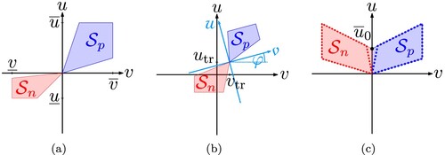
The approach is initially illustrated using the ZCS depicted in Figure 4(a). Let the convex subset in the first and third quadrant be given by (29a) $\begin{array}{rl}{S}_p& \left\{\left(u,v\right)|u\in U,v\in V,{\widehat{\mathbf{\text{h}}}}_{\mathrm{z}\mathrm{c}\mathrm{s},p}(u,v)\le \mathbf{\text{0}}\right\}\mathrm{a}\mathrm{n}\mathrm{d}\end{array}$(29a) (29b) $\begin{array}{rl}{S}_n& \left\{\left(u,v\right)|u\in U,v\in V,{\widehat{\mathbf{\text{h}}}}_{\mathrm{z}\mathrm{c}\mathrm{s},n}(u,v)\le \mathbf{\text{0}}\right\},\end{array}$(29b) respectively. Therein v and u are original decision variables. Moreover, ${\widehat{\mathbf{\text{h}}}}_{\mathrm{z}\mathrm{c}\mathrm{s},p}\le \mathbf{\text{0}}$ and ${\widehat{\mathbf{\text{h}}}}_{\mathrm{z}\mathrm{c}\mathrm{s},n}\le \mathbf{\text{0}}$ are convex sets. The union of convex sets does not necessarily result in a convex set. As illustrated in Figure 4(a), the union $S=S_p\cup S_n$ is assumed to be nonconvex in this article. Thus, $S$ is a nonconvex set comprised of convex subsets: a ZCS. The velocity v is split at $v=v_{\mathrm{t}\mathrm{r}}=0$ by a vertical line following Lemma 2.1. The two auxiliary variables $v_n\in V_n[\underset{\_}{v},v_{\mathrm{t}\mathrm{r}}]=[\underset{\_}{v},0]$ and $v_p\in V_p[v_{\mathrm{t}\mathrm{r}},\overline{v}]=[0,\overline{v}]$ are introduced aiming at implementing (30) $\begin{array}{r}{v}_n=\left\{\begin{array}{ll}v& \mathrm{\forall }v\le 0,\\ 0& \mathrm{e}\mathrm{l}\mathrm{s}\mathrm{e}\end{array}\right.\mathrm{a}\mathrm{n}\mathrm{d}{v}_p=\left\{\begin{array}{ll}v& \mathrm{\forall }v\ge 0,\\ 0& \mathrm{e}\mathrm{l}\mathrm{s}\mathrm{e}\end{array}\right..\end{array}$(30)

Introducing analogous constraints to (9a(9a) $\begin{array}{rl}{g}_{\text{aff}}& =w_{\text{up}}+w_{\text{low}}-(w+w_{\text{tr}})=0\end{array}$(9a) ) and (11a(11a) $\begin{array}{r}{g}_{\mathrm{a}\mathrm{b}\mathrm{s}}=w_{-2\$\mathrm{\Delta }\$}-|\tilde{w}|\ge 0\iff {\mathbf{\text{h}}}_{\mathrm{a}\mathrm{b}\mathrm{s}}=\left[\begin{array}{c}{w}_{-2\$\mathrm{\Delta }\$}-\tilde{w}\\ w_{-2\$\mathrm{\Delta }\$}+\tilde{w}\end{array}\right]\ge \mathbf{\text{0}}.\end{array}$(11a) ) as well as additional objective terms in form of (11c(11c) $\begin{array}{rl}& J_g\tau l_{\mathrm{a}\mathrm{b}\mathrm{s}}\end{array}$(11c) ) ensures the relations in (30(30) $\begin{array}{r}{v}_n=\left\{\begin{array}{ll}v& \mathrm{\forall }v\le 0,\\ 0& \mathrm{e}\mathrm{l}\mathrm{s}\mathrm{e}\end{array}\right.\mathrm{a}\mathrm{n}\mathrm{d}{v}_p=\left\{\begin{array}{ll}v& \mathrm{\forall }v\ge 0,\\ 0& \mathrm{e}\mathrm{l}\mathrm{s}\mathrm{e}\end{array}\right..\end{array}$(30) ). Furthermore, the auxiliary variables $u_n\in U_n[\underset{\_}{u},u_{\mathrm{t}\mathrm{r}}]$ and $u_p\in U_p[u_{\mathrm{t}\mathrm{r}},\overline{u}]$ are introduced for the individual subsets. Therein $u_{\mathrm{t}\mathrm{r}}$ represents the ordinate value of the common point, which lies on the origin in the current example depicted in Figure 4(a) resulting in $u_{\mathrm{t}\mathrm{r}}=0$. However, the common point of the subsets is not required to lie on the abscissa or ordinate. The vector of auxiliary decision variables is given by ${\mathbf{\text{w}}}_{\mathrm{a}\mathrm{u}\mathrm{x}}=\left[\begin{array}{cccc}{v}_p& v_n& u_p& u_n\end{array}\right]$. While the original state variable v remains a decision variable in the problem, the input variable is replaced according to the transformation (31) $\begin{array}{r}{\mathrm{\Phi }}_u{u}_n+u_p-u_{\mathrm{t}\mathrm{r}}=\left[\begin{array}{cc}1& 1\end{array}\right]\left[\begin{array}{c}{u}_p\\ u_n\end{array}\right]-u_{\mathrm{t}\mathrm{r}},\end{array}$(31) which is affine in the decision variables. The convex subsets in terms of the auxiliary decision variables are given by (32a) $\begin{array}{rl}{\hat{S}}_p& \left\{\left(u_p,v_p\right)|u_p\in U_p,v_p\in V_p,{\widehat{\mathbf{\text{h}}}}_{\mathrm{z}\mathrm{c}\mathrm{s},p}(u_p,v_p)\le \mathbf{\text{0}}\right\}\end{array}$(32a) (32b) $\begin{array}{rl}{\hat{S}}_n& \left\{\left(u_n,v_n\right)|u_n\in U_n,v_n\in V_n,{\widehat{\mathbf{\text{h}}}}_{\mathrm{z}\mathrm{c}\mathrm{s},n}(u_n,v_n)\le \mathbf{\text{0}}\right\}.\end{array}$(32b) Hence, the convex subsets ${\hat{S}}_p$ and ${\hat{S}}_n$ are now defined for separate decision variables and will be linked via the affine mapping (31(31) $\begin{array}{r}{\mathrm{\Phi }}_u{u}_n+u_p-u_{\mathrm{t}\mathrm{r}}=\left[\begin{array}{cc}1& 1\end{array}\right]\left[\begin{array}{c}{u}_p\\ u_n\end{array}\right]-u_{\mathrm{t}\mathrm{r}},\end{array}$(31) ). This enables the formulation of convex constraints as depicted in problem (15(15a) $\begin{array}{rl}\underset{\mathbf{\text{z}}}{min}& J\left(\mathbf{\text{w}}\right)\end{array}$(15a) ). The proof that this procedure produces the same set as $S$ will be given in Theorem 2.3.

For convexity, ${\widehat{\mathbf{\text{h}}}}_{\mathrm{z}\mathrm{c}\mathrm{s},p}$ and ${\widehat{\mathbf{\text{h}}}}_{\mathrm{z}\mathrm{c}\mathrm{s},n}$ in (32a(32a) $\begin{array}{rl}{\hat{S}}_p& \left\{\left(u_p,v_p\right)|u_p\in U_p,v_p\in V_p,{\widehat{\mathbf{\text{h}}}}_{\mathrm{z}\mathrm{c}\mathrm{s},p}(u_p,v_p)\le \mathbf{\text{0}}\right\}\end{array}$(32a) ) and (32b(32b) $\begin{array}{rl}{\hat{S}}_n& \left\{\left(u_n,v_n\right)|u_n\in U_n,v_n\in V_n,{\widehat{\mathbf{\text{h}}}}_{\mathrm{z}\mathrm{c}\mathrm{s},n}(u_n,v_n)\le \mathbf{\text{0}}\right\}.\end{array}$(32b) ) must be convex functions. As exemplarily illustrated in Figure 4(a), the convex subsets are assumed in this article to be representable by $n_{\mathrm{z}\mathrm{c}\mathrm{s}}=n_{\mathrm{z}\mathrm{c}\mathrm{s},n}+n_{\mathrm{z}\mathrm{c}\mathrm{s},p}$ affine inequality constraints (33a) $\begin{array}{r}{\widehat{\mathbf{\text{h}}}}_{\mathrm{z}\mathrm{c}\mathrm{s},p}(u,v){\mathbf{\text{A}}}_{\mathrm{z}\mathrm{c}\mathrm{s},p}\left[\begin{array}{c}u\\ v\end{array}\right]+{\mathbf{\text{b}}}_{\mathrm{z}\mathrm{c}\mathrm{s},p}\le \mathbf{\text{0}}\end{array}$(33a) (33b) $\begin{array}{r}{\widehat{\mathbf{\text{h}}}}_{\mathrm{z}\mathrm{c}\mathrm{s},n}(u,v){\mathbf{\text{A}}}_{\mathrm{z}\mathrm{c}\mathrm{s},n}\left[\begin{array}{c}u\\ v\end{array}\right]+{\mathbf{\text{b}}}_{\mathrm{z}\mathrm{c}\mathrm{s},n}\le \mathbf{\text{0}}\end{array}$(33b) with ${\mathbf{\text{A}}}_{\mathrm{z}\mathrm{c}\mathrm{s},p}\in {\mathbb{R}}^{n_{\mathrm{z}\mathrm{c}\mathrm{s},p}\times 2}$, ${\mathbf{\text{b}}}_{\mathrm{z}\mathrm{c}\mathrm{s},p}\in {\mathbb{R}}^{n_{\mathrm{z}\mathrm{c}\mathrm{s},p}}$, ${\mathbf{\text{A}}}_{\mathrm{z}\mathrm{c}\mathrm{s},n}\in {\mathbb{R}}^{n_{\mathrm{z}\mathrm{c}\mathrm{s},n}\times 2}$ and ${\mathbf{\text{b}}}_{\mathrm{z}\mathrm{c}\mathrm{s},n}\in {\mathbb{R}}^{n_{\mathrm{z}\mathrm{c}\mathrm{s},n}}$. These constraints represent (15e(15e) $\begin{array}{rl}& {\widehat{\mathbf{\text{h}}}}_{\mathrm{z}\mathrm{c}\mathrm{s},k}\left(\mathbf{\text{z}}\right)\le \mathbf{\text{0}},\end{array}$(15e) ) in the convex OP. Although nonlinear, convex functions for ${\widehat{\mathbf{\text{h}}}}_{\mathrm{z}\mathrm{c}\mathrm{s},p}$ and ${\widehat{\mathbf{\text{h}}}}_{\mathrm{z}\mathrm{c}\mathrm{s},n}$ would not prevent convexity, introducing such constraints would prohibit an LP or QP problem, which can be solved especially efficiently. Asymmetric subsets like the one illustrated in Figure 4(a) can be easily implemented by using varying coefficients in (33a(33a) $\begin{array}{r}{\widehat{\mathbf{\text{h}}}}_{\mathrm{z}\mathrm{c}\mathrm{s},p}(u,v){\mathbf{\text{A}}}_{\mathrm{z}\mathrm{c}\mathrm{s},p}\left[\begin{array}{c}u\\ v\end{array}\right]+{\mathbf{\text{b}}}_{\mathrm{z}\mathrm{c}\mathrm{s},p}\le \mathbf{\text{0}}\end{array}$(33a) ) and (33b(33b) $\begin{array}{r}{\widehat{\mathbf{\text{h}}}}_{\mathrm{z}\mathrm{c}\mathrm{s},n}(u,v){\mathbf{\text{A}}}_{\mathrm{z}\mathrm{c}\mathrm{s},n}\left[\begin{array}{c}u\\ v\end{array}\right]+{\mathbf{\text{b}}}_{\mathrm{z}\mathrm{c}\mathrm{s},n}\le \mathbf{\text{0}}\end{array}$(33b) ) or by using different domains for $U_n$ and $U_p$.

Theorem 2.3

The subsets (32a(32a) $\begin{array}{rl}{\hat{S}}_p& \left\{\left(u_p,v_p\right)|u_p\in U_p,v_p\in V_p,{\widehat{\mathbf{\text{h}}}}_{\mathrm{z}\mathrm{c}\mathrm{s},p}(u_p,v_p)\le \mathbf{\text{0}}\right\}\end{array}$(32a) ) and (32b(32b) $\begin{array}{rl}{\hat{S}}_n& \left\{\left(u_n,v_n\right)|u_n\in U_n,v_n\in V_n,{\widehat{\mathbf{\text{h}}}}_{\mathrm{z}\mathrm{c}\mathrm{s},n}(u_n,v_n)\le \mathbf{\text{0}}\right\}.\end{array}$(32b) ) in combination with the affine mapping (31(31) $\begin{array}{r}{\mathrm{\Phi }}_u{u}_n+u_p-u_{\mathrm{t}\mathrm{r}}=\left[\begin{array}{cc}1& 1\end{array}\right]\left[\begin{array}{c}{u}_p\\ u_n\end{array}\right]-u_{\mathrm{t}\mathrm{r}},\end{array}$(31) ) depict the set $S$ which is given by the union of the convex subsets (29a(29a) $\begin{array}{rl}{S}_p& \left\{\left(u,v\right)|u\in U,v\in V,{\widehat{\mathbf{\text{h}}}}_{\mathrm{z}\mathrm{c}\mathrm{s},p}(u,v)\le \mathbf{\text{0}}\right\}\mathrm{a}\mathrm{n}\mathrm{d}\end{array}$(29a) ) and (29b(29b) $\begin{array}{rl}{S}_n& \left\{\left(u,v\right)|u\in U,v\in V,{\widehat{\mathbf{\text{h}}}}_{\mathrm{z}\mathrm{c}\mathrm{s},n}(u,v)\le \mathbf{\text{0}}\right\},\end{array}$(29b) ).

Proof.

For proving that the splitting approach provides sets that depict the original one, the individual cases for the bisected variable space are considered subsequently.

Case 1: $v_{\mathrm{t}\mathrm{r}}<v$

The decision variable v is split at $v=v_{\mathrm{t}\mathrm{r}}$. Thus, $v_n=v_{\mathrm{t}\mathrm{r}}$ holds according to Lemma 2.1. This concludes $u_n=u_{\mathrm{t}\mathrm{r}}$ since the subsets converge to the common point $(u_{\mathrm{t}\mathrm{r}},v_{\mathrm{t}\mathrm{r}})$ when leaving the subset towards the other subset. Lemma 2.1 also concludes $v_p=v$. Then, the affine mapping (31(31) $\begin{array}{r}{\mathrm{\Phi }}_u{u}_n+u_p-u_{\mathrm{t}\mathrm{r}}=\left[\begin{array}{cc}1& 1\end{array}\right]\left[\begin{array}{c}{u}_p\\ u_n\end{array}\right]-u_{\mathrm{t}\mathrm{r}},\end{array}$(31) ) is given by ${\mathrm{\Phi }}_u=u_p\in {\hat{S}}_p$. For $v>v_{\mathrm{t}\mathrm{r}}$, $S=S_p$ holds. Since $v_p=v$, $u\in S_p$ and ${\mathrm{\Phi }}_u\in {\hat{S}}_p$ provide the same feasible set. The chain of conclusions for the remaining cases follows the same reasoning but is given below in equations for conciseness.

Case 2: $v<v_{\mathrm{t}\mathrm{r}}$ (34a) $\begin{array}{r}\left.\begin{array}{c}{v}_p=v_{\mathrm{t}\mathrm{r}}\Rightarrow u_p=u_{\mathrm{t}\mathrm{r}}\\ v_n=v\end{array}\right\}\Rightarrow {\mathrm{\Phi }}_u=u_n\in {\hat{S}}_n\widehat{=}u\in S=S_n.\end{array}$(34a) Case 3: $v=v_{\mathrm{t}\mathrm{r}}$ (34b) $\begin{array}{r}\left.\begin{array}{c}{v}_p=v_{\mathrm{t}\mathrm{r}}\Rightarrow u_p=u_{\mathrm{t}\mathrm{r}}\\ v_n=v_{\mathrm{t}\mathrm{r}}\Rightarrow u_n=u_{\mathrm{t}\mathrm{r}}\end{array}\right\}\Rightarrow {\mathrm{\Phi }}_u=u_{\mathrm{t}\mathrm{r}}\widehat{=}u=u_{\mathrm{t}\mathrm{r}}.\end{array}$(34b)

Thus, inserting the affine mapping (31(31) $\begin{array}{r}{\mathrm{\Phi }}_u{u}_n+u_p-u_{\mathrm{t}\mathrm{r}}=\left[\begin{array}{cc}1& 1\end{array}\right]\left[\begin{array}{c}{u}_p\\ u_n\end{array}\right]-u_{\mathrm{t}\mathrm{r}},\end{array}$(31) ) into the constraints while replacing the original set $S$ with the sets (32a(32a) $\begin{array}{rl}{\hat{S}}_p& \left\{\left(u_p,v_p\right)|u_p\in U_p,v_p\in V_p,{\widehat{\mathbf{\text{h}}}}_{\mathrm{z}\mathrm{c}\mathrm{s},p}(u_p,v_p)\le \mathbf{\text{0}}\right\}\end{array}$(32a) ) and (32b(32b) $\begin{array}{rl}{\hat{S}}_n& \left\{\left(u_n,v_n\right)|u_n\in U_n,v_n\in V_n,{\widehat{\mathbf{\text{h}}}}_{\mathrm{z}\mathrm{c}\mathrm{s},n}(u_n,v_n)\le \mathbf{\text{0}}\right\}.\end{array}$(32b) ) yields the same feasible set.

The presented proof requires a space splitting of the variable v which is represented by splitting the convex subsets via a vertical line. Thus, the SSC approach is capable of convexifying two-dimensional ZCSs, which can be divided into two convex subsets connected in a single point using any vertical line. Following theorem is added to show that this also holds for any splitting line which is straight but possibly rotated:

Theorem 2.4

Space splitting applied to a rotated, two-dimensional ZCS also results in convex constraints.

Proof.

This can be verified by applying the previously described procedure to a rotated coordinate frame, exemplarily depicted in Figure 4(b). The auxiliary decision variables need to split the rotated two-dimensional space spanned by the variables $\mathcal{v}$ and $\mathcal{u}$. Assuming the coordinate system is rotated by the angle φ with counter-clockwise rotations depicting positive rotations, following relations hold between the original coordinates v−u and the rotated coordinates $\mathcal{v}-\mathcal{u}$: (35) $\begin{array}{r}\begin{array}{rl}\left[\begin{array}{c}\mathcal{v}\\ \mathcal{u}\end{array}\right]& =\underset{\mathrm{R}\left(\phi \right)}{\underbrace{\left[\begin{array}{cc}\cos \left(\phi \right)& \sin \left(\phi \right)\\ -\sin \left(\phi \right)& \cos \left(\phi \right)\end{array}\right]}}\left[\begin{array}{c}v-v_{\mathrm{t}\mathrm{r}}\\ u-u_{\mathrm{t}\mathrm{r}}\end{array}\right]\mathrm{a}\mathrm{n}\mathrm{d}\\ \left[\begin{array}{c}v\\ u\end{array}\right]& =\underset{\mathrm{R}(-\phi )}{\underbrace{\left[\begin{array}{cc}\cos \left(\phi \right)& -\sin \left(\phi \right)\\ \sin \left(\phi \right)& \cos \left(\phi \right)\end{array}\right]}}\left[\begin{array}{c}\mathcal{v}\\ \mathcal{u}\end{array}\right]+\left[\begin{array}{c}{v}_{\mathrm{t}\mathrm{r}}\\ u_{\mathrm{t}\mathrm{r}}\end{array}\right].\end{array}\end{array}$(35) The vector of auxiliary decision variables is chosen as ${\mathbf{\text{w}}}_{\mathrm{a}\mathrm{u}\mathrm{x}}=\left[\begin{array}{cccc}{\mathcal{v}}_p& {\mathcal{v}}_n& {\mathcal{u}}_p& {\mathcal{u}}_n\end{array}\right]$. For a concise notation, the equations below use the abbreviations ${\mathrm{c}}_{\phi }\cos \left(\phi \right)$ and ${\mathrm{s}}_{\phi }\sin \left(\phi \right)$. Constraints (33(33a) $\begin{array}{r}{\widehat{\mathbf{\text{h}}}}_{\mathrm{z}\mathrm{c}\mathrm{s},p}(u,v){\mathbf{\text{A}}}_{\mathrm{z}\mathrm{c}\mathrm{s},p}\left[\begin{array}{c}u\\ v\end{array}\right]+{\mathbf{\text{b}}}_{\mathrm{z}\mathrm{c}\mathrm{s},p}\le \mathbf{\text{0}}\end{array}$(33a) ) are analogously formulated on the rotated, auxiliary decision variables: ${\widehat{\mathbf{\text{h}}}}_{\mathrm{z}\mathrm{c}\mathrm{s},p}({\mathcal{u}}_p,{\mathcal{v}}_p)$ and ${\widehat{\mathbf{\text{h}}}}_{\mathrm{z}\mathrm{c}\mathrm{s},n}({\mathcal{u}}_n,{\mathcal{v}}_n)$. However, an adjustment using (35(35) $\begin{array}{r}\begin{array}{rl}\left[\begin{array}{c}\mathcal{v}\\ \mathcal{u}\end{array}\right]& =\underset{\mathrm{R}\left(\phi \right)}{\underbrace{\left[\begin{array}{cc}\cos \left(\phi \right)& \sin \left(\phi \right)\\ -\sin \left(\phi \right)& \cos \left(\phi \right)\end{array}\right]}}\left[\begin{array}{c}v-v_{\mathrm{t}\mathrm{r}}\\ u-u_{\mathrm{t}\mathrm{r}}\end{array}\right]\mathrm{a}\mathrm{n}\mathrm{d}\\ \left[\begin{array}{c}v\\ u\end{array}\right]& =\underset{\mathrm{R}(-\phi )}{\underbrace{\left[\begin{array}{cc}\cos \left(\phi \right)& -\sin \left(\phi \right)\\ \sin \left(\phi \right)& \cos \left(\phi \right)\end{array}\right]}}\left[\begin{array}{c}\mathcal{v}\\ \mathcal{u}\end{array}\right]+\left[\begin{array}{c}{v}_{\mathrm{t}\mathrm{r}}\\ u_{\mathrm{t}\mathrm{r}}\end{array}\right].\end{array}\end{array}$(35) ) is necessary for the constraints (9a(9a) $\begin{array}{rl}{g}_{\text{aff}}& =w_{\text{up}}+w_{\text{low}}-(w+w_{\text{tr}})=0\end{array}$(9a) ), (11a(11a) $\begin{array}{r}{g}_{\mathrm{a}\mathrm{b}\mathrm{s}}=w_{-2\$\mathrm{\Delta }\$}-|\tilde{w}|\ge 0\iff {\mathbf{\text{h}}}_{\mathrm{a}\mathrm{b}\mathrm{s}}=\left[\begin{array}{c}{w}_{-2\$\mathrm{\Delta }\$}-\tilde{w}\\ w_{-2\$\mathrm{\Delta }\$}+\tilde{w}\end{array}\right]\ge \mathbf{\text{0}}.\end{array}$(11a) ) and (11b(11b) $\begin{array}{rl}{l}_{\mathrm{a}\mathrm{b}\mathrm{s}}& =w_{-2\$\mathrm{\Delta }\$}-{\sigma }_w\tilde{w}=0,{\sigma }_w\mathrm{s}\mathrm{i}\mathrm{g}\mathrm{n}\left({\tilde{w}}^{\star }\right)=\mathrm{s}\mathrm{i}\mathrm{g}\mathrm{n}(w_{\mathrm{p}\mathrm{r}\mathrm{e}\mathrm{v}}^{\star }-w_{\mathrm{t}\mathrm{r}})\end{array}$(11b) ) as well as the input mapping (31(31) $\begin{array}{r}{\mathrm{\Phi }}_u{u}_n+u_p-u_{\mathrm{t}\mathrm{r}}=\left[\begin{array}{cc}1& 1\end{array}\right]\left[\begin{array}{c}{u}_p\\ u_n\end{array}\right]-u_{\mathrm{t}\mathrm{r}},\end{array}$(31) ): (36a) $\begin{array}{r}\begin{array}{rl}{g}_{\mathrm{a}\mathrm{f}\mathrm{f}}& =({\mathcal{v}}_p+{\mathcal{v}}_n)-\tilde{\mathcal{v}}=0\text{with}\\ \tilde{\mathcal{v}}& ={\mathrm{c}}_{\phi }(v-v_{\mathrm{t}\mathrm{r}})+{\mathrm{s}}_{\phi }({\mathrm{s}}_{\phi }({\mathcal{v}}_p+{\mathcal{v}}_n)+{\mathrm{c}}_{\phi }({\mathcal{u}}_p+{\mathcal{u}}_n))\end{array}\end{array}$(36a) (36b) $\begin{array}{rl}{g}_{\mathrm{a}\mathrm{b}\mathrm{s}}& =({\mathcal{v}}_p-{\mathcal{v}}_n)-|\tilde{\mathcal{v}}|\ge 0\end{array}$(36b) (36c) $\begin{array}{rl}{l}_{\mathrm{a}\mathrm{b}\mathrm{s}}& =({\mathcal{v}}_p-{\mathcal{v}}_n)-\mathrm{s}\mathrm{i}\mathrm{g}\mathrm{n}\left(\tilde{\mathcal{v}}\right)\tilde{\mathcal{v}}\ge 0\end{array}$(36c) (36d) $\begin{array}{rl}{\mathrm{\Phi }}_u& =u=\left[\begin{array}{cc}{\mathrm{s}}_{\phi }& {\mathrm{s}}_{\phi }\end{array}\right]\left[\begin{array}{c}{\mathcal{v}}_p\\ {\mathcal{v}}_n\end{array}\right]+\left[\begin{array}{cc}{\mathrm{c}}_{\phi }& {\mathrm{c}}_{\phi }\end{array}\right]\left[\begin{array}{c}{\mathcal{u}}_p\\ {\mathcal{u}}_n\end{array}\right]+u_{\mathrm{t}\mathrm{r}}.\end{array}$(36d) Since the angle φ is constant, the trigonometric functions represent constant values. Thus, a rotated space splitting procedure also yields affine constraints and mappings enabling the formulation of a convex OP.

The previous theorems required the subsets to be connected in a single point. Following theorem states that the SSC approach can be used to approximate ZCSs which share a line of points:

Theorem 2.5

When a two-dimensional ZCSs is comprised of two convex subsets sharing a line of points, the SSC approach can only approximate the original set however with sufficiently small approximation error.

Proof.

Without loss of generality, this can be analysed considering Figure 4(c) as example. For the depicted case, the transition line lies on the ordinate $v_{\mathrm{t}\mathrm{r}}=0$. Analysing the individual cases shows that using the original subsets within the SSC approach would yield a larger set than the original set:

Case 1: $v_{\mathrm{t}\mathrm{r}}<v$ (37a) $\begin{array}{rl}\left.\begin{array}{c}{v}_p=v\Rightarrow u_p\in {\hat{S}}_p\\ v_n=v_{\mathrm{t}\mathrm{r}}\Rightarrow u_n\in [0,{\overline{u}}_0]\end{array}\right\}\Rightarrow {\mathrm{\Phi }}_u& =(u_n+u_p)\in {\hat{S}}_{\mathrm{\Phi },p}\supset {\hat{S}}_p\\ & \widehat{=}u\in S=S_p.\end{array}$(37a)

Case 2: $v<v_{\mathrm{t}\mathrm{r}}$ (37b) $\begin{array}{rl}\left.\begin{array}{c}{v}_p=v_{\mathrm{t}\mathrm{r}}\Rightarrow u_p\in [0,{\overline{u}}_0]\\ v_n=v\Rightarrow u_n\in {\hat{S}}_n\end{array}\right\}\Rightarrow {\mathrm{\Phi }}_u& =(u_n+u_p)\in {\hat{S}}_{\mathrm{\Phi },n}\supset {\hat{S}}_n\\ & \widehat{=}u\in S=S_n.\end{array}$(37b)

Case 3: $v=v_{\mathrm{t}\mathrm{r}}$ (37c) $\begin{array}{rl}\left.\begin{array}{c}{v}_p=v_{\mathrm{t}\mathrm{r}}\Rightarrow u_p\in [0,{\overline{u}}_0]\\ v_n=v_{\mathrm{t}\mathrm{r}}\Rightarrow u_n\in [0,{\overline{u}}_0]\end{array}\right\}\Rightarrow {\mathrm{\Phi }}_u& =u_n+u_p\in [0,2{\overline{u}}_0]\\ & \widehat{=}u\in [0,{\overline{u}}_0].\end{array}$(37c)

Thus, using the original subsets can render non-admissible points of the original problem admissible. When the input variable is replaced by the auxiliary inputs according to (31(31) $\begin{array}{r}{\mathrm{\Phi }}_u{u}_n+u_p-u_{\mathrm{t}\mathrm{r}}=\left[\begin{array}{cc}1& 1\end{array}\right]\left[\begin{array}{c}{u}_p\\ u_n\end{array}\right]-u_{\mathrm{t}\mathrm{r}},\end{array}$(31) ), both sets must be adjusted at the transition line $v=v_{\mathrm{t}\mathrm{r}}$. The simplest set adjustment is enforcing $u_n=0=u_p$ at the transition axis, as illustrated in Figure 4c by the dotted lines. Then, the subsets are connected in a single point enabling the application of Theorem 2.4. However, other set manipulations are possible and can be numerically better. Generally, such set approximations introduce conservativeness for the sake of feasible trajectories. However, the introduced error is negligible when the removed area is sufficiently small which can be implemented by choosing steep linear constraints at the transition between the subsets.

Remark 2.2

In this article, only two-dimensional ZCSs which can be split into two convex subsets have been considered. However, the SSC approach can be applied to certain two-dimensional ZCSs with more than two subsets. For instance, consider three convex subsets positioned horizontally to each other, whereas each subset is connected to the next subset in a single point on the abscissa. This can be verified using the procedures described previously in this section.

This section illustrated the convexification procedure for ZCSs in regards to inputs. This results in the depicted affine input transformation ${\mathrm{\Phi }}_u$. Implementing the approach for a ZCS with state decision variables yields an affine transformation ${\mathrm{\Phi }}_x$. This procedure can be applied to multiple inputs and states. The corresponding vector functions for the affine transformations are given by (38) $\begin{array}{r}{\mathbf{\Phi }}_u=\left[\begin{array}{c}{\mathrm{\Phi }}_{u,1}\\ ⋮\\ {\mathrm{\Phi }}_{u,n_u}\end{array}\right]\mathrm{a}\mathrm{n}\mathrm{d}{\mathbf{\Phi }}_x=\left[\begin{array}{c}{\mathrm{\Phi }}_{x,1}\\ ⋮\\ {\mathrm{\Phi }}_{x,n_x}\end{array}\right]\end{array}$(38) with ${\mathrm{\Phi }}_{u,i}$ and ${\mathrm{\Phi }}_{x,j}$ representing the transformation for the individual input and state, respectively. If no transformation is necessary, a direct mapping is implemented according to ${\mathrm{\Phi }}_{u,i}=u_i$ and ${\mathrm{\Phi }}_{x,i}=x_i$. The vectors of transformations (38(38) $\begin{array}{r}{\mathbf{\Phi }}_u=\left[\begin{array}{c}{\mathrm{\Phi }}_{u,1}\\ ⋮\\ {\mathrm{\Phi }}_{u,n_u}\end{array}\right]\mathrm{a}\mathrm{n}\mathrm{d}{\mathbf{\Phi }}_x=\left[\begin{array}{c}{\mathrm{\Phi }}_{x,1}\\ ⋮\\ {\mathrm{\Phi }}_{x,n_x}\end{array}\right]\end{array}$(38) ) are used to generate $\mathbf{\Phi }$ in (17(17) $\begin{array}{rl}\mathbf{\text{w}}=\mathbf{\Phi }\left(\mathbf{\text{z}}\right)=\left[\begin{array}{c}{\mathbf{\Phi }}_0\\ ⋮\\ {\mathbf{\Phi }}_{n_{\mathrm{s}\mathrm{e}\mathrm{g}}}\end{array}\right]\widehat{\mathbf{\text{A}}}\mathbf{\text{z}}+\widehat{\mathbf{\text{b}}},{\mathbf{\Phi }}_k& \left[\begin{array}{c}{\mathbf{\Phi }}_x{\mid }_k\\ {\mathbf{\Phi }}_u{\mid }_k\end{array}\right]\end{array}$(17) ) which is used for the convex depiction of the original constraints in (15b(15b) $\begin{array}{rl}\mathrm{s}.\mathrm{t}.& {\widehat{\mathbf{\text{c}}}}_{\mathrm{c}\mathrm{o}\mathrm{l}\mathrm{l},i}\left(\mathbf{\text{z}}\right)={\mathbf{\text{c}}}_{\mathrm{c}\mathrm{o}\mathrm{l}\mathrm{l},i}(\mathbf{\text{w}}=\mathbf{\Phi }(\mathbf{\text{z}}),{\mathbf{\text{f}}}_{\mathrm{p}\mathrm{w}\mathrm{l}}={\mathbf{\Phi }}_{\mathrm{p}\mathrm{w}\mathrm{l}})=\mathbf{\text{0}},\end{array}$(15b) )–(15d(15d) $\begin{array}{rl}& {\widehat{\mathbf{\text{h}}}}_k\left(\mathbf{\text{z}}\right)={\mathbf{\text{h}}}_k(\mathbf{\text{w}}=\mathbf{\Phi }(\mathbf{\text{z}}\left)\right)\le \mathbf{\text{0}},\end{array}$(15d) ).

2.3.2. Convexification of nonlinear equality constraints

Some nonlinearities in physical systems are characterised by a univariate function. Examples are nonlinear springs, saturation, dead-zones or the tire force shape curve of vehicles. Since nonlinear system equations yield nonlinear thus nonconvex equality constraints, this section presents how such nonlinear univariate terms can be convexified. The nonlinear univariate curve is depicted using piecewise affine parts. Hence, if the nonlinearity is not a piecewise linear function, SSC introduces approximation errors. The subsequent paragraphs illustrate the application of the SSC algorithm for convexifying piecewise linear nonlinearities.

Theorem 2.6

The splitting constraints in (9(9a) $\begin{array}{rl}{g}_{\text{aff}}& =w_{\text{up}}+w_{\text{low}}-(w+w_{\text{tr}})=0\end{array}$(9a) ) can be used to convexify equality constraints by transforming a univariate nonlinearity with two piecewise linear segments into an expression which is affine in multiple decision variables.

Proof.

Proof is provided using the piecewise linear curve depicted in Figure 5(a) as example, which represents a typical function for piecewise linear springs. Assuming the position x is a state of the system, it represents a decision variable which will be split at the transition point $x=x_{\mathrm{t}\mathrm{r}}<0$. Thus, the auxiliary position variables $x_{\mathrm{l}\mathrm{o}\mathrm{w}}\in X_{\mathrm{l}\mathrm{o}\mathrm{w}}[\underset{\_}{x},x_{\mathrm{t}\mathrm{r}}]$ and $x_{\mathrm{u}\mathrm{p}}\in X_{\mathrm{u}\mathrm{p}}[x_{\mathrm{t}\mathrm{r}},\overline{x}]$ are introduced. By including analogous constraints to (9a(9a) $\begin{array}{rl}{g}_{\text{aff}}& =w_{\text{up}}+w_{\text{low}}-(w+w_{\text{tr}})=0\end{array}$(9a) ) and (11a(11a) $\begin{array}{r}{g}_{\mathrm{a}\mathrm{b}\mathrm{s}}=w_{-2\$\mathrm{\Delta }\$}-|\tilde{w}|\ge 0\iff {\mathbf{\text{h}}}_{\mathrm{a}\mathrm{b}\mathrm{s}}=\left[\begin{array}{c}{w}_{-2\$\mathrm{\Delta }\$}-\tilde{w}\\ w_{-2\$\mathrm{\Delta }\$}+\tilde{w}\end{array}\right]\ge \mathbf{\text{0}}.\end{array}$(11a) ) as well as additional objective terms in form of (11c(11c) $\begin{array}{rl}& J_g\tau l_{\mathrm{a}\mathrm{b}\mathrm{s}}\end{array}$(11c) ), following relations are ensured using Lemma 2.1: (39) $\begin{array}{r}{x}_{\mathrm{l}\mathrm{o}\mathrm{w}}=\left\{\begin{array}{ll}x& \mathrm{\forall }x\le x_{\mathrm{t}\mathrm{r}},\\ x_{\mathrm{t}\mathrm{r}}& \mathrm{e}\mathrm{l}\mathrm{s}\mathrm{e}\end{array}\right.,x_{\mathrm{u}\mathrm{p}}=\left\{\begin{array}{ll}x& \mathrm{\forall }x\ge x_{\mathrm{t}\mathrm{r}},\\ x_{\mathrm{t}\mathrm{r}}& \mathrm{e}\mathrm{l}\mathrm{s}\mathrm{e}\end{array}\right..\end{array}$(39) Hence, the piecewise linear function can be represented by the expression (40) $\begin{array}{rl}{\mathrm{\Phi }}_{\mathrm{p}\mathrm{w}\mathrm{l},2}& =c_{\mathrm{u}\mathrm{p}}{x}_{\mathrm{u}\mathrm{p}}+c_{\mathrm{l}\mathrm{o}\mathrm{w}}(x_{\mathrm{l}\mathrm{o}\mathrm{w}}-x_{\mathrm{t}\mathrm{r}})\\ & =\left[\begin{array}{cc}{c}_{\mathrm{u}\mathrm{p}}& c_{\mathrm{l}\mathrm{o}\mathrm{w}}\end{array}\right]\underset{{\mathbf{\text{w}}}_{\mathrm{a}\mathrm{u}\mathrm{x}}}{\underbrace{\left[\begin{array}{c}{x}_{\mathrm{u}\mathrm{p}}\\ x_{\mathrm{l}\mathrm{o}\mathrm{w}}\end{array}\right]}}+\left(-c_{\mathrm{l}\mathrm{o}\mathrm{w}}{x}_{\mathrm{t}\mathrm{r}}\right)\end{array}$(40) which is affine in the decision variables ${\mathbf{\text{w}}}_{\mathrm{a}\mathrm{u}\mathrm{x}}$. The relations in (39(39) $\begin{array}{r}{x}_{\mathrm{l}\mathrm{o}\mathrm{w}}=\left\{\begin{array}{ll}x& \mathrm{\forall }x\le x_{\mathrm{t}\mathrm{r}},\\ x_{\mathrm{t}\mathrm{r}}& \mathrm{e}\mathrm{l}\mathrm{s}\mathrm{e}\end{array}\right.,x_{\mathrm{u}\mathrm{p}}=\left\{\begin{array}{ll}x& \mathrm{\forall }x\ge x_{\mathrm{t}\mathrm{r}},\\ x_{\mathrm{t}\mathrm{r}}& \mathrm{e}\mathrm{l}\mathrm{s}\mathrm{e}\end{array}\right..\end{array}$(39) ) yield following two segments for the piecewise linear function (40(40) $\begin{array}{rl}{\mathrm{\Phi }}_{\mathrm{p}\mathrm{w}\mathrm{l},2}& =c_{\mathrm{u}\mathrm{p}}{x}_{\mathrm{u}\mathrm{p}}+c_{\mathrm{l}\mathrm{o}\mathrm{w}}(x_{\mathrm{l}\mathrm{o}\mathrm{w}}-x_{\mathrm{t}\mathrm{r}})\\ & =\left[\begin{array}{cc}{c}_{\mathrm{u}\mathrm{p}}& c_{\mathrm{l}\mathrm{o}\mathrm{w}}\end{array}\right]\underset{{\mathbf{\text{w}}}_{\mathrm{a}\mathrm{u}\mathrm{x}}}{\underbrace{\left[\begin{array}{c}{x}_{\mathrm{u}\mathrm{p}}\\ x_{\mathrm{l}\mathrm{o}\mathrm{w}}\end{array}\right]}}+\left(-c_{\mathrm{l}\mathrm{o}\mathrm{w}}{x}_{\mathrm{t}\mathrm{r}}\right)\end{array}$(40) ): (41a) $\begin{array}{rl}& \mathrm{I}:x_{\mathrm{t}\mathrm{r}}\le x\Rightarrow \left\{\begin{array}{l}{x}_{\mathrm{u}\mathrm{p}}=x\\ x_{\mathrm{l}\mathrm{o}\mathrm{w}}=x_{\mathrm{t}\mathrm{r}}\end{array}\right.\Rightarrow {\mathrm{\Phi }}_{\mathrm{p}\mathrm{w}\mathrm{l},2}=c_{\mathrm{u}\mathrm{p}}x.\end{array}$(41a) (41b) $\begin{array}{rl}\mathrm{I}\mathrm{I}:x<x_{\mathrm{t}\mathrm{r}}& \Rightarrow \left\{\begin{array}{l}{x}_{\mathrm{u}\mathrm{p}}=x_{\mathrm{t}\mathrm{r}}\\ x_{\mathrm{l}\mathrm{o}\mathrm{w}}=x\end{array}\right.\\ & \Rightarrow {\mathrm{\Phi }}_{\mathrm{p}\mathrm{w}\mathrm{l},2}=c_{\mathrm{u}\mathrm{p}}{x}_{\mathrm{t}\mathrm{r}}+c_{\mathrm{l}\mathrm{o}\mathrm{w}}(x-x_{\mathrm{t}\mathrm{r}}).\end{array}$(41b) Thus, (41a(41a) $\begin{array}{rl}& \mathrm{I}:x_{\mathrm{t}\mathrm{r}}\le x\Rightarrow \left\{\begin{array}{l}{x}_{\mathrm{u}\mathrm{p}}=x\\ x_{\mathrm{l}\mathrm{o}\mathrm{w}}=x_{\mathrm{t}\mathrm{r}}\end{array}\right.\Rightarrow {\mathrm{\Phi }}_{\mathrm{p}\mathrm{w}\mathrm{l},2}=c_{\mathrm{u}\mathrm{p}}x.\end{array}$(41a) ) and (41b(41b) $\begin{array}{rl}\mathrm{I}\mathrm{I}:x<x_{\mathrm{t}\mathrm{r}}& \Rightarrow \left\{\begin{array}{l}{x}_{\mathrm{u}\mathrm{p}}=x_{\mathrm{t}\mathrm{r}}\\ x_{\mathrm{l}\mathrm{o}\mathrm{w}}=x\end{array}\right.\\ & \Rightarrow {\mathrm{\Phi }}_{\mathrm{p}\mathrm{w}\mathrm{l},2}=c_{\mathrm{u}\mathrm{p}}{x}_{\mathrm{t}\mathrm{r}}+c_{\mathrm{l}\mathrm{o}\mathrm{w}}(x-x_{\mathrm{t}\mathrm{r}}).\end{array}$(41b) ) depict the upper and lower segment of the nonlinearity, respectively.

Since (40(40) $\begin{array}{rl}{\mathrm{\Phi }}_{\mathrm{p}\mathrm{w}\mathrm{l},2}& =c_{\mathrm{u}\mathrm{p}}{x}_{\mathrm{u}\mathrm{p}}+c_{\mathrm{l}\mathrm{o}\mathrm{w}}(x_{\mathrm{l}\mathrm{o}\mathrm{w}}-x_{\mathrm{t}\mathrm{r}})\\ & =\left[\begin{array}{cc}{c}_{\mathrm{u}\mathrm{p}}& c_{\mathrm{l}\mathrm{o}\mathrm{w}}\end{array}\right]\underset{{\mathbf{\text{w}}}_{\mathrm{a}\mathrm{u}\mathrm{x}}}{\underbrace{\left[\begin{array}{c}{x}_{\mathrm{u}\mathrm{p}}\\ x_{\mathrm{l}\mathrm{o}\mathrm{w}}\end{array}\right]}}+\left(-c_{\mathrm{l}\mathrm{o}\mathrm{w}}{x}_{\mathrm{t}\mathrm{r}}\right)\end{array}$(40) ) is an affine function in the decision variables, it can be inserted into the differential equations without preventing convexity. The subsequent theorem proves that this approach can be extended to univariate nonlinearities with more than two piecewise linear segments:

Figure 5. Space splitting convexification of piecewise linear equalities. (a) Nonlinearity with two linear segments. (b) Nonlinearity with three linear segments. (c) Splitting of state variable x for three segments.

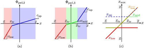
Theorem 2.7

A repeated application of the space bisection approach using the splitting constraints in (9(9a) $\begin{array}{rl}{g}_{\text{aff}}& =w_{\text{up}}+w_{\text{low}}-(w+w_{\text{tr}})=0\end{array}$(9a) ) can be used to convexify equality constraints by transforming a univariate nonlinearity with more than two piecewise linear segments into an expression which is affine in multiple decision variables.

Proof.

The general procedure for this extension is illustrated using the piecewise linear curve depicted in Figure 5(b). The position x is split at the transition points $x={\underset{\_}{x}}_{\mathrm{t}\mathrm{r}}<0$ and $x={\overline{x}}_{\mathrm{t}\mathrm{r}}>0$. Thus, the auxiliary position variables $x_{\mathrm{l}\mathrm{o}\mathrm{w}}\in X_{\mathrm{l}\mathrm{o}\mathrm{w}}[\underset{\_}{x},{\underset{\_}{x}}_{\mathrm{t}\mathrm{r}}]$, $x_{\overline{\mathrm{l}\mathrm{o}\mathrm{w}}}\in X_{\overline{\mathrm{l}\mathrm{o}\mathrm{w}}}[{\underset{\_}{x}}_{\mathrm{t}\mathrm{r}},\overline{x}]$, $x_{\mathrm{m}\mathrm{i}\mathrm{d}}\in X_{\mathrm{m}\mathrm{i}\mathrm{d}}[{\underset{\_}{x}}_{\mathrm{t}\mathrm{r}},{\overline{x}}_{\mathrm{t}\mathrm{r}}]$ and $x_{\mathrm{u}\mathrm{p}}\in X_{\mathrm{u}\mathrm{p}}[{\overline{x}}_{\mathrm{t}\mathrm{r}},\overline{x}]$ are employed. The space is repeatedly bisected following Lemma 2.1 to gain (42a) $\begin{array}{rl}{x}_{\mathrm{l}\mathrm{o}\mathrm{w}}& =\left\{\begin{array}{ll}x& \mathrm{\forall }x\le {\underset{\_}{x}}_{\mathrm{t}\mathrm{r}},\\ {\underset{\_}{x}}_{\mathrm{t}\mathrm{r}}& \mathrm{e}\mathrm{l}\mathrm{s}\mathrm{e}\end{array}\right.,x_{\overline{\mathrm{l}\mathrm{o}\mathrm{w}}}=\left\{\begin{array}{ll}x& \mathrm{\forall }x\ge {\underset{\_}{x}}_{\mathrm{t}\mathrm{r}},\\ {\underset{\_}{x}}_{\mathrm{t}\mathrm{r}}& \mathrm{e}\mathrm{l}\mathrm{s}\mathrm{e}\end{array}\right.\end{array}$(42a) (42b) $\begin{array}{rl}{x}_{\mathrm{m}\mathrm{i}\mathrm{d}}& =\left\{\begin{array}{ll}{x}_{\overline{\mathrm{l}\mathrm{o}\mathrm{w}}}& \mathrm{\forall }{x}_{\overline{\mathrm{l}\mathrm{o}\mathrm{w}}}\le {\overline{x}}_{\mathrm{t}\mathrm{r}},\\ {\overline{x}}_{\mathrm{t}\mathrm{r}}& \mathrm{e}\mathrm{l}\mathrm{s}\mathrm{e}\end{array}\right.,x_{\mathrm{u}\mathrm{p}}=\left\{\begin{array}{ll}{x}_{\overline{\mathrm{l}\mathrm{o}\mathrm{w}}}& \mathrm{\forall }{x}_{\overline{\mathrm{l}\mathrm{o}\mathrm{w}}}\ge {\overline{x}}_{\mathrm{t}\mathrm{r}},\\ {\overline{x}}_{\mathrm{t}\mathrm{r}}& \mathrm{e}\mathrm{l}\mathrm{s}\mathrm{e}\end{array}\right.\end{array}$(42b) which is depicted in Figure 5. Thus, the position space is bisected into a region below and a region above $x={\underset{\_}{x}}_{\mathrm{t}\mathrm{r}}$ whereas the upper region is again bisected into a region below and above $x={\overline{x}}_{\mathrm{t}\mathrm{r}}$. The piecewise linear function can then be represented by the expression (43) $\begin{array}{r}{\mathrm{\Phi }}_{\mathrm{p}\mathrm{w}\mathrm{l},3}=\left[\begin{array}{ccc}{c}_{\mathrm{u}\mathrm{p}}& c_{\mathrm{m}\mathrm{i}\mathrm{d}}& c_{\mathrm{l}\mathrm{o}\mathrm{w}}\end{array}\right]\underset{{\mathbf{\text{w}}}_{\mathrm{a}\mathrm{u}\mathrm{x}}}{\underbrace{\left[\begin{array}{c}{x}_{\mathrm{u}\mathrm{p}}\\ x_{\mathrm{m}\mathrm{i}\mathrm{d}}\\ x_{\mathrm{l}\mathrm{o}\mathrm{w}}\end{array}\right]}}-(c_{\mathrm{u}\mathrm{p}}{\overline{x}}_{\mathrm{t}\mathrm{r}}+c_{\mathrm{l}\mathrm{o}\mathrm{w}}{\underset{\_}{x}}_{\mathrm{t}\mathrm{r}})\end{array}$(43) which is affine in the decision variables ${\mathbf{\text{w}}}_{\mathrm{a}\mathrm{u}\mathrm{x}}$. The relations in (42(42a) $\begin{array}{rl}{x}_{\mathrm{l}\mathrm{o}\mathrm{w}}& =\left\{\begin{array}{ll}x& \mathrm{\forall }x\le {\underset{\_}{x}}_{\mathrm{t}\mathrm{r}},\\ {\underset{\_}{x}}_{\mathrm{t}\mathrm{r}}& \mathrm{e}\mathrm{l}\mathrm{s}\mathrm{e}\end{array}\right.,x_{\overline{\mathrm{l}\mathrm{o}\mathrm{w}}}=\left\{\begin{array}{ll}x& \mathrm{\forall }x\ge {\underset{\_}{x}}_{\mathrm{t}\mathrm{r}},\\ {\underset{\_}{x}}_{\mathrm{t}\mathrm{r}}& \mathrm{e}\mathrm{l}\mathrm{s}\mathrm{e}\end{array}\right.\end{array}$(42a) ) yield following three segments for the piecewise linear function (43(43) $\begin{array}{r}{\mathrm{\Phi }}_{\mathrm{p}\mathrm{w}\mathrm{l},3}=\left[\begin{array}{ccc}{c}_{\mathrm{u}\mathrm{p}}& c_{\mathrm{m}\mathrm{i}\mathrm{d}}& c_{\mathrm{l}\mathrm{o}\mathrm{w}}\end{array}\right]\underset{{\mathbf{\text{w}}}_{\mathrm{a}\mathrm{u}\mathrm{x}}}{\underbrace{\left[\begin{array}{c}{x}_{\mathrm{u}\mathrm{p}}\\ x_{\mathrm{m}\mathrm{i}\mathrm{d}}\\ x_{\mathrm{l}\mathrm{o}\mathrm{w}}\end{array}\right]}}-(c_{\mathrm{u}\mathrm{p}}{\overline{x}}_{\mathrm{t}\mathrm{r}}+c_{\mathrm{l}\mathrm{o}\mathrm{w}}{\underset{\_}{x}}_{\mathrm{t}\mathrm{r}})\end{array}$(43) ): (44a) $\begin{array}{rl}\mathrm{I}:{\overline{x}}_{\mathrm{t}\mathrm{r}}<x& \Rightarrow \left\{\begin{array}{l}{x}_{\mathrm{u}\mathrm{p}}=x\\ x_{\mathrm{m}\mathrm{i}\mathrm{d}}={\overline{x}}_{\mathrm{t}\mathrm{r}}\\ x_{\mathrm{l}\mathrm{o}\mathrm{w}}={\underset{\_}{x}}_{\mathrm{t}\mathrm{r}}\end{array}\right.\\ & \Rightarrow {\mathrm{\Phi }}_{\mathrm{p}\mathrm{w}\mathrm{l},3}=c_{\mathrm{m}\mathrm{i}\mathrm{d}}{\overline{x}}_{\mathrm{t}\mathrm{r}}+c_{\mathrm{u}\mathrm{p}}(x-{\overline{x}}_{\mathrm{t}\mathrm{r}}).\end{array}$(44a) (44b) $\begin{array}{rl}\mathrm{I}\mathrm{I}:{\underset{\_}{x}}_{\mathrm{t}\mathrm{r}}\le x\le {\overline{x}}_{\mathrm{t}\mathrm{r}}& \Rightarrow \left\{\begin{array}{l}{x}_{\mathrm{u}\mathrm{p}}={\overline{x}}_{\mathrm{t}\mathrm{r}}\\ x_{\mathrm{m}\mathrm{i}\mathrm{d}}=x\\ x_{\mathrm{l}\mathrm{o}\mathrm{w}}={\underset{\_}{x}}_{\mathrm{t}\mathrm{r}}\end{array}\right.\\ & \Rightarrow {\mathrm{\Phi }}_{\mathrm{p}\mathrm{w}\mathrm{l},3}=c_{\mathrm{m}\mathrm{i}\mathrm{d}}x.\end{array}$(44b) (44c) $\begin{array}{rl}\mathrm{I}\mathrm{I}\mathrm{I}:x<{\underset{\_}{x}}_{\mathrm{t}\mathrm{r}}& \Rightarrow \left\{\begin{array}{l}{x}_{\mathrm{u}\mathrm{p}}={\overline{x}}_{\mathrm{t}\mathrm{r}}\\ x_{\mathrm{m}\mathrm{i}\mathrm{d}}={\underset{\_}{x}}_{\mathrm{t}\mathrm{r}}\\ x_{\mathrm{l}\mathrm{o}\mathrm{w}}=x\end{array}\right.\\ & \Rightarrow {\mathrm{\Phi }}_{\mathrm{p}\mathrm{w}\mathrm{l},3}=c_{\mathrm{m}\mathrm{i}\mathrm{d}}{\underset{\_}{x}}_{\mathrm{t}\mathrm{r}}+c_{\mathrm{l}\mathrm{o}\mathrm{w}}(x-{\underset{\_}{x}}_{\mathrm{t}\mathrm{r}}).\end{array}$(44c) Hence, (44a(44a) $\begin{array}{rl}\mathrm{I}:{\overline{x}}_{\mathrm{t}\mathrm{r}}<x& \Rightarrow \left\{\begin{array}{l}{x}_{\mathrm{u}\mathrm{p}}=x\\ x_{\mathrm{m}\mathrm{i}\mathrm{d}}={\overline{x}}_{\mathrm{t}\mathrm{r}}\\ x_{\mathrm{l}\mathrm{o}\mathrm{w}}={\underset{\_}{x}}_{\mathrm{t}\mathrm{r}}\end{array}\right.\\ & \Rightarrow {\mathrm{\Phi }}_{\mathrm{p}\mathrm{w}\mathrm{l},3}=c_{\mathrm{m}\mathrm{i}\mathrm{d}}{\overline{x}}_{\mathrm{t}\mathrm{r}}+c_{\mathrm{u}\mathrm{p}}(x-{\overline{x}}_{\mathrm{t}\mathrm{r}}).\end{array}$(44a) ), (44b(44b) $\begin{array}{rl}\mathrm{I}\mathrm{I}:{\underset{\_}{x}}_{\mathrm{t}\mathrm{r}}\le x\le {\overline{x}}_{\mathrm{t}\mathrm{r}}& \Rightarrow \left\{\begin{array}{l}{x}_{\mathrm{u}\mathrm{p}}={\overline{x}}_{\mathrm{t}\mathrm{r}}\\ x_{\mathrm{m}\mathrm{i}\mathrm{d}}=x\\ x_{\mathrm{l}\mathrm{o}\mathrm{w}}={\underset{\_}{x}}_{\mathrm{t}\mathrm{r}}\end{array}\right.\\ & \Rightarrow {\mathrm{\Phi }}_{\mathrm{p}\mathrm{w}\mathrm{l},3}=c_{\mathrm{m}\mathrm{i}\mathrm{d}}x.\end{array}$(44b) ) and (44c(44c) $\begin{array}{rl}\mathrm{I}\mathrm{I}\mathrm{I}:x<{\underset{\_}{x}}_{\mathrm{t}\mathrm{r}}& \Rightarrow \left\{\begin{array}{l}{x}_{\mathrm{u}\mathrm{p}}={\overline{x}}_{\mathrm{t}\mathrm{r}}\\ x_{\mathrm{m}\mathrm{i}\mathrm{d}}={\underset{\_}{x}}_{\mathrm{t}\mathrm{r}}\\ x_{\mathrm{l}\mathrm{o}\mathrm{w}}=x\end{array}\right.\\ & \Rightarrow {\mathrm{\Phi }}_{\mathrm{p}\mathrm{w}\mathrm{l},3}=c_{\mathrm{m}\mathrm{i}\mathrm{d}}{\underset{\_}{x}}_{\mathrm{t}\mathrm{r}}+c_{\mathrm{l}\mathrm{o}\mathrm{w}}(x-{\underset{\_}{x}}_{\mathrm{t}\mathrm{r}}).\end{array}$(44c) ) depict the upper, mid and lower segment of the nonlinearity, respectively.

This repeated bisection procedure enables the generation of a characteristic curve with an arbitrary number of segments. However, an increasing number of segments also increases the number of auxiliary decision variables and additional constraints making the OP larger.

The approach presented in this section yields a scalar function ${\mathrm{\Phi }}_{\mathrm{p}\mathrm{w}\mathrm{l}}$ which is affine in the decision variables. The procedure can be applied to multiple univariate, nonlinear terms yielding further scalar mapping functions. The affine vector-valued function in (16(16) $\begin{array}{r}\begin{array}{rl}{\mathbf{\text{f}}}_{\mathrm{\Phi }}(\mathbf{\text{x}},\mathbf{\text{u}},{\mathbf{\text{w}}}_{\mathrm{a}\mathrm{u}\mathrm{x}})=& \left(\mathbf{\text{A}}{\mathbf{\Phi }}_x(\mathbf{\text{x}},\mathbf{\text{u}},{\mathbf{\text{w}}}_{\mathrm{a}\mathrm{u}\mathrm{x}})+\mathbf{\text{B}}{\mathbf{\Phi }}_u(\mathbf{\text{x}},\mathbf{\text{u}},{\mathbf{\text{w}}}_{\mathrm{a}\mathrm{u}\mathrm{x}})+\mathbf{\text{k}}\right)+\\ & +{\mathbf{\Phi }}_{\mathrm{p}\mathrm{w}\mathrm{l}}(\mathbf{\text{x}},\mathbf{\text{u}},{\mathbf{\text{w}}}_{\mathrm{a}\mathrm{u}\mathrm{x}})\end{array}\end{array}$(16) ) is given by (45) $\begin{array}{r}{\mathbf{\Phi }}_{\mathrm{p}\mathrm{w}\mathrm{l}}=\left[\begin{array}{c}{\mathrm{\Phi }}_{\mathrm{p}\mathrm{w}\mathrm{l},1,1}+{\mathrm{\Phi }}_{\mathrm{p}\mathrm{w}\mathrm{l},1,2}+\dots \\ ⋮\\ {\mathrm{\Phi }}_{\mathrm{p}\mathrm{w}\mathrm{l},n_x,1}+{\mathrm{\Phi }}_{\mathrm{p}\mathrm{w}\mathrm{l},n_x,2}+\dots \end{array}\right]\end{array}$(45) with ${\mathrm{\Phi }}_{\mathrm{p}\mathrm{w}\mathrm{l},i,j}$ representing the individual affine mapping functions. For states that are not affected by the space splitting approach, ${\mathrm{\Phi }}_{\mathrm{p}\mathrm{w}\mathrm{l},i,j}=0$ holds. The transformation (45(45) $\begin{array}{r}{\mathbf{\Phi }}_{\mathrm{p}\mathrm{w}\mathrm{l}}=\left[\begin{array}{c}{\mathrm{\Phi }}_{\mathrm{p}\mathrm{w}\mathrm{l},1,1}+{\mathrm{\Phi }}_{\mathrm{p}\mathrm{w}\mathrm{l},1,2}+\dots \\ ⋮\\ {\mathrm{\Phi }}_{\mathrm{p}\mathrm{w}\mathrm{l},n_x,1}+{\mathrm{\Phi }}_{\mathrm{p}\mathrm{w}\mathrm{l},n_x,2}+\dots \end{array}\right]\end{array}$(45) ) is used to generate the convex collocation constraints (15b(15b) $\begin{array}{rl}\mathrm{s}.\mathrm{t}.& {\widehat{\mathbf{\text{c}}}}_{\mathrm{c}\mathrm{o}\mathrm{l}\mathrm{l},i}\left(\mathbf{\text{z}}\right)={\mathbf{\text{c}}}_{\mathrm{c}\mathrm{o}\mathrm{l}\mathrm{l},i}(\mathbf{\text{w}}=\mathbf{\Phi }(\mathbf{\text{z}}),{\mathbf{\text{f}}}_{\mathrm{p}\mathrm{w}\mathrm{l}}={\mathbf{\Phi }}_{\mathrm{p}\mathrm{w}\mathrm{l}})=\mathbf{\text{0}},\end{array}$(15b) ).

2.4. Remarks on runtime

The application of optimisation methods within a real-time capable controller generally requires upper bounds on the necessary computation time. The SSC approach runs through a loop which is comprised of a projection step and an optimisation step resulting in the following theorem regarding computational complexity:

Theorem 2.8

The computational complexity of the SSC algorithm is polynomial.

Proof.

SSC solves a sequence of LP problems or convex QP problems, which are known to be solvable in polynomial time (Karmarkar, 1984; Kozlov et al., 1980). The projection step (12(12) $\begin{array}{r}\breve{w}=w_{\mathrm{p}\mathrm{r}\mathrm{e}\mathrm{v}}^{\star },{\breve{w}}_{\mathrm{l}\mathrm{o}\mathrm{w}}=min(w_{\mathrm{p}\mathrm{r}\mathrm{e}\mathrm{v}}^{\star },w_{\mathrm{t}\mathrm{r}}),{\breve{w}}_{\mathrm{u}\mathrm{p}}=max(w_{\mathrm{p}\mathrm{r}\mathrm{e}\mathrm{v}}^{\star },w_{\mathrm{t}\mathrm{r}}).\end{array}$(12) ) of the SSC algorithm uses minimum and maximum functions which possess linear time complexity. This concludes a polynomial time complexity of the SSC algorithm: (46) $\begin{array}{r}{T}_{\mathrm{S}\mathrm{S}\mathrm{C}}(n,q)=q\cdot \left(O\left(n^{\alpha }\right)+cO\left(n\right)\right)\mathrm{w}\mathrm{i}\mathrm{t}\mathrm{h}\alpha >1.\end{array}$(46) Therein n can be interpreted as the number of operations required by the algorithm. The parameters in (46(46) $\begin{array}{r}{T}_{\mathrm{S}\mathrm{S}\mathrm{C}}(n,q)=q\cdot \left(O\left(n^{\alpha }\right)+cO\left(n\right)\right)\mathrm{w}\mathrm{i}\mathrm{t}\mathrm{h}\alpha >1.\end{array}$(46) ) depend on the utilised solver as well as the number of decision variables which is problem specific. Limiting the maximum number of superordinate iterations to $q\le q_{\mathrm{m}\mathrm{a}\mathrm{x}}$ enables terminating the algorithm prematurely at suboptimal solutions, if necessary.

Theorem 2.8 provides valuable insight for the application in a real-time capable controller. Firstly, a worst-case bound on computation time can be experimentally identified for the specific OP and solver. Secondly, the computation time scales well with increasing problem size. Since the number of superordinate SSC iterations is rather low in practice, this results in a fast solution of optimal control problems. Finally, the influences on computation time are summarised below:

1. System and discretisation. The number of decision variables increases with rising number of inputs, states and collocation segments for both the original and the convexified OP. This increases computation time for NLP methods and the SSC algorithm. Due to the polynomial complexity, this increase in time will be generally less for SSC than for NLP.

2. Nonlinearity. The more complicated the nonlinearity, the more splitting segments are required to reduce approximation errors. However, the space splitting increases the problem size compared to the original problem, which influences the variable n in (46(46) $\begin{array}{r}{T}_{\mathrm{S}\mathrm{S}\mathrm{C}}(n,q)=q\cdot \left(O\left(n^{\alpha }\right)+cO\left(n\right)\right)\mathrm{w}\mathrm{i}\mathrm{t}\mathrm{h}\alpha >1.\end{array}$(46) ). This can put a practical bound on the number of space divisions via the SSC approach. Nevertheless, many physically motivated nonlinearities can be approximated sufficiently well using a moderate number of affine segments.

3. Initial guess. Being a local method, the solution computed by the SSC approach depends on the provided initial solution. Furthermore, this initial guess can influence the order of sign-corrections regarding the AVC-linearisations, which can impact the number of superordinate iterations and, therefore, the convergence rate. For MPC frameworks, the optimal solution of the preceding time step often represents a good initial guess (Gros et al., 2020) promising low computation times.

4. Penalty parameter update. Too small or too large penalty parameters can slow down convergence (Nocedal & Wright, 2006, p. 511). The straightforward approach of gradually increasing the penalty parameter is used in this article. However, more sophisticated routines have been proposed in Mayne and Maratos (1979) and Maratos (1978).

2.5. Comparison with existing methods

In order to highlight the novelty of the proposed algorithm, this section compares the SSC approach with the most related existing methods.

From an algorithmic standpoint, linearising only the nonconvex part of constraints combined with a relaxation and an increasing objective term penalising constraint violations corresponds to penalty CCP (Lipp & Boyd, 2016). CCP has the advantage over SQP and other linearisation techniques that it retains more problem information in each iterate: The information of the convex parts is kept and only the concave portions are linearised. Furthermore, CCP does not require to use line-search procedures or limit the progress in each iteration via trust-region methods. Inspired by Mangasarian (2015), the SSC approach avoids additional slack variables by considering the linearised constraints directly in the penalty objective. This avoids further increasing the size of the OP as in penalty CCP. Moreover, SSC employs an intermediate projection to enhance convergence. While CCP linearises the concave part of all nonconvexities, SSC transforms the problem beforehand requiring only the linearisation of AVCs. This enables providing a feedback about the correctness of the selected linearisation points, which are subsequently adjusted. Thus, the linearisation error can vanish completely after the correct signs have been chosen. The binary nature of the linearisation facilitates a rapid convergence in a small number of superordinate iterations. Although the SSC method only computes solutions to the piecewise linear approximation of the original problem, the approximation can be designed to sufficient accuracy enabling small and known approximation errors. Especially the straightforward linearisation of ZCS-constraints yields very poor approximations, which can contain a large set of infeasible points. Thus, the vanishing AVC-linearisation errors result in an advantage of SSC regarding accuracy, also over further linearisation techniques like the ones presented in Mao et al. ( 2016, 2017). Generally, a scalable trade-off between accuracy and size of the OP, thus computation time, can be chosen. Opposed to Lipp and Boyd (2016), this article provides a convergence proof, even if only converging to the solution of the approximated problem.

While LC possesses the advantage of avoiding approximation errors, it is only applicable to OPs with annulus-like, nonconvex sets resulting from excluding a convex subset from a convex set (Raković & Levine, 2018, p. 340). Opposed to that, SSC provides a method for the convexification of ZCS which cannot be considered via LC.

Similar to the LnP approach presented in Mao et al. (2017), the SSC method is an iterative linearisation algorithm using intermediate projection steps. The updating routine for SSC is of linear computational complexity with few and simple mathematical operations. The projection step of the LnP approach generally requires the solution of a convex programming problem, which is of polynomial complexity at best. Thus, the projection step used by the SSC approach is computationally less costly, which is beneficial for splitting methods (Ferreau et al., 2017). Additionally, the binary nature of the AVC-linearisation provides the advantage that generally only few superordinate iterations are required, resulting in short computation times. Moreover, SSC is more robust regarding the initialisation since the LnP approach requires an additional lifting procedure to cope with arbitrary initialisations, which costs computation time (Mao et al., 2017). Furthermore, the LnP method requires the right-hand side of the system equations to be convex and the inequality constraints to be concave. However, nonconvex collision avoidance constraints can be easily considered via the LnP approach, whereas the SSC procedure requires further measures.

The ADMM is a splitting procedure utilising the augmented Lagrangian method instead of the exact penalty function method, which is employed by the SSC algorithm. Due to the alternating approach, the ADMM requires the solution of two QCQP problems in each iteration. The SSC approach only requires the solution of a single convex QP problem in each iteration, which is beneficial for computation time.

The spatial BnB method also uses space decomposition for the convexification of the optimisation problem. However, the SSC approach solves a piecewise linear approximation of the original problem, which is iteratively adjusted, on the full space domain of the decision variables. Opposed to that, the BnB method solves multiple OPs which represent convexly relaxed versions of the original problem on separate subdomains of the decision variables. BnB techniques determine upper bounds by evaluating the objective function at a feasible point. Since the problem is generally nonconvex, finding a feasible point can be difficult. This is often tackled by solving the nonconvex subproblem locally, which is computationally expensive (Liberti & Maculan, 2006, p. 253). Thus, the convergence rate of the SSC approach is most likely to be superior if sufficiently good initial guesses are provided. However, this depends on the nonlinearities of the OP, which influence the number of decision variables for SSC but also for BnB approaches which decompose factorable functions (Tawarmalani & Sahinidis, 2002, p. 125). Moreover, SSC only guarantees to find local optima of an approximation of the OP and is only applicable to certain classes of OPs. GO techniques cover a wide range of applicability and provide the global optimum.

3. Applications

In this section, the proposed SSC algorithm is evaluated using a hanging SMO example with piecewise linear spring and semi-active damping as illustrated in Figure 6. Semi-active dampers can only generate a force in the opposite moving direction and cannot impose a force at steady-state complying with the passivity constraint (Savaresi et al., 2010, p. 16). Hence, the admissible set for semi-active dampers always contains a subset in the first quadrant and a subset in the third quadrant which are connected in a single point, namely, the origin. A performance-oriented OP is formulated and solved using NLP and SSC, respectively. The results of both algorithms are compared regarding accuracy and computation time. Both problems are posed using the modelling language JuMP (Dunning et al., 2017) for mathematical OPs. For a fair comparison, the necessary derivatives are computed beforehand via automatic differentiation. Furthermore, the tolerances for constraint feasibility and objective improvement are set to ${10}^{-6}$ for both solvers. The utilised parameters are listed with description in Table 1.

Figure 6. Model characteristics for hanging SMO with semi-active damper and nonlinear spring. (a) Hanging SMO model. (b) ZCS for semi-active damper force. (c) Piecewise linear spring force characteristic.

Table 1. Parameters for SMO application.

Symbol	Value	Unit	Description
g	9.81	m/${\mathrm{s}}^2$	gravitational acceleration
m	5.00	kg	mass
$c_{\mathrm{u}\mathrm{p}}$	10.00	N/m	overload spring stiffness for rebound
$c_{\mathrm{m}\mathrm{i}\mathrm{d}}$	3.00	N/m	main spring stiffness
$c_{\mathrm{l}\mathrm{o}\mathrm{w}}$	5.00	N/m	overload spring stiffness for compression
${\overline{x}}_{\mathrm{t}\mathrm{r}}$	5.00	m	transition point for rebound overload
${\underset{\_}{x}}_{\mathrm{t}\mathrm{r}}$	$-5.00$	m	transition point for compression overload
$x_{\mathrm{s}\mathrm{s},2}$	16.35	m	steady-state position for 2-segment spring
$x_{\mathrm{s}\mathrm{s},3}$	8.405	m	steady-state position for 3-segment spring
$\overline{x}$	100.00	m	upper position bound
$\underset{\_}{x}$	$-100.00$	m	lower position bound
$\overline{d}$	20.00	Ns/m	upper bound on damper coefficient
$\underset{\_}{d}$	0.50	Ns/m	lower bound on damper coefficient
$\overline{v}$	100.00	m/s	upper speed bound
$\underset{\_}{v}$	$-100.00$	m/s	lower speed bound
${\overline{F}}_d$	400.00	N	upper bound on damper force
${\underset{\_}{F}}_d$	$-400.00$	N	lower bound on damper force
${ϵ}_g$	${10}^{-6}$	–	violation tolerance for SSC penalty term
$\underset{\_}{\tau }/\overline{\tau }$	$1.00/{10}^4$	–	initial/final value for penalty parameter

The NLP problem is solved using the optimiser IPOPT(Wächter & Biegler, 2006), which employs an interior-point method: Using the concept of barrier functions, a sequence of relaxed problems is solved for decreasing values of barrier parameters. The barrier parameter relaxes the inequality constraints and hence represents the distance from the current iterate to the border of the admissible set. Thus, interior-point methods use a central path within the admissible set as opposed to SQP-methods which wander along the border. The resulting nonlinear equation system is solved via a damped Newton method. Furthermore, a filter line-search method, heuristics and further correction measures are employed to enhance convergence and robustness.

The novel SSC method transforms the OP into convex QP subproblems which are solved iteratively. In order to capitalise on this problem structure, the elaborate optimiser Gurobi (Gurobi Optimization, 2020) is selected.

3.1. Optimisation problems

The equations of motion for the state vector $\mathbf{\text{x}}=[xv{]}^{\mathrm{T}}$ result in (47) $\begin{array}{r}\dot{\mathbf{\text{x}}}=\mathbf{\text{f}}=\left[\begin{array}{c}v\\ \frac{1}{m}\left(mg-F_d-F_c\right)\end{array}\right]\end{array}$(47) with x, v, $F_d$ and $F_c$ denoting the deflection position, deflection speed, damper force and spring force, respectively. The expression of these forces differs for the NLP method and the SSC approach. Starting from a specified initial state ${\mathbf{\text{x}}}_{\mathrm{i}\mathrm{v}}=[x_{\mathrm{i}\mathrm{v}}{v}_{\mathrm{i}\mathrm{v}}{]}^{\mathrm{T}}$ with damper force $F_{d,\mathrm{i}\mathrm{v}}=\underset{\_}{d}{v}_{\mathrm{i}\mathrm{v}}$, the goal is to minimise the deviation from the steady-state position $x_{\mathrm{s}\mathrm{s}}$ while considering the limitations of the system. Applying Simpson quadrature (Betts, 2010; Kelly, 2017), the main objective penalises the steady-state position deviation $e_{\mathrm{s}\mathrm{s},j}{x}_j-x_{\mathrm{s}\mathrm{s}}$ according to (48) $\begin{array}{r}{J}_{\mathrm{s}\mathrm{s}}\sum _{i=0}^{n_{\mathrm{s}\mathrm{e}\mathrm{g}}-1}\frac{{\mathrm{\Delta }}_i}{6}\left(e_{\mathrm{s}\mathrm{s},i}^2+4e_{\mathrm{s}\mathrm{s},i+\frac{1}{2}}^2+e_{\mathrm{s}\mathrm{s},i+1}^2\right).\end{array}$(48) Considering the values listed in Table 1, the steady-state position can be computed using a root-finding approach like Newton's method: At steady-state position, the gravitational force must equal the spring force. For the considered nonlinear springs with two piecewise linear segments the value $x_{\mathrm{s}\mathrm{s}}=x_{\mathrm{s}\mathrm{s},2}$ is chosen and $x_{\mathrm{s}\mathrm{s}}=x_{\mathrm{s}\mathrm{s},3}$ if the spring with three segments is used. An uniform discretisation of the time grid $t\in [t_0,t_f]=[0,10]$ is employed yielding a constant segment width ${\mathrm{\Delta }}_i=\mathrm{\Delta }=\frac{t_f-t_0}{n_{\mathrm{s}\mathrm{e}\mathrm{g}}}$. Both, the NLP approach and the SSC method, are initialised with zero vectors ${\mathbf{\text{U}}}_0^{\star }=\mathbf{\text{0}}$ and ${\mathbf{\text{X}}}_0^{\star }=\mathbf{\text{0}}$. From (49) $\begin{array}{rl}{f}_{\mathrm{s}\mathrm{s},i}\left(x\right)& \frac{{\mathrm{\Delta }}_i}{6}(x_i-x_{\mathrm{s}\mathrm{s}}{)}^2\Rightarrow f_{\mathrm{s}\mathrm{s},i}^{\prime }(x)=2\frac{{\mathrm{\Delta }}_i}{6}(x_i-x_{\mathrm{s}\mathrm{s}})\\ & \Rightarrow f_{\mathrm{s}\mathrm{s},i}^{″}\left(x\right)=2\frac{{\mathrm{\Delta }}_i}{6}>0\end{array}$(49) follows that the Hessian of (48(48) $\begin{array}{r}{J}_{\mathrm{s}\mathrm{s}}\sum _{i=0}^{n_{\mathrm{s}\mathrm{e}\mathrm{g}}-1}\frac{{\mathrm{\Delta }}_i}{6}\left(e_{\mathrm{s}\mathrm{s},i}^2+4e_{\mathrm{s}\mathrm{s},i+\frac{1}{2}}^2+e_{\mathrm{s}\mathrm{s},i+1}^2\right).\end{array}$(48) ) is a diagonal matrix with only positive and zero diagonal entries and therefore positive semi-definite. Hence, the main objective (48(48) $\begin{array}{r}{J}_{\mathrm{s}\mathrm{s}}\sum _{i=0}^{n_{\mathrm{s}\mathrm{e}\mathrm{g}}-1}\frac{{\mathrm{\Delta }}_i}{6}\left(e_{\mathrm{s}\mathrm{s},i}^2+4e_{\mathrm{s}\mathrm{s},i+\frac{1}{2}}^2+e_{\mathrm{s}\mathrm{s},i+1}^2\right).\end{array}$(48) ) is a convex function.

3.1.1. Nonlinear nonconvex optimisation problem

For the solution of the OP via NLP, the decision variables are chosen as (50a) $\begin{array}{rl}\mathbf{\text{u}}& =\left[\begin{array}{cccc}{u}_0& u_{0.5}& \dots & u_{n_{\mathrm{s}\mathrm{e}\mathrm{g}}}\end{array}\right]\in {\mathbb{R}}^{1\times n_{\mathrm{p}\mathrm{t}\mathrm{s}}}\text{with}{u}_k=d_k\end{array}$(50a) (50b) $\begin{array}{rl}\mathbf{\text{X}}& =\left[\begin{array}{cccc}{\mathbf{\text{x}}}_0& {\mathbf{\text{x}}}_{0.5}& \dots & {\mathbf{\text{x}}}_{n_{\mathrm{s}\mathrm{e}\mathrm{g}}}\end{array}\right]\in {\mathbb{R}}^{2\times n_{\mathrm{p}\mathrm{t}\mathrm{s}}}\mathrm{w}\mathrm{i}\mathrm{t}\mathrm{h}{\mathbf{\text{x}}}_k\left[\begin{array}{c}{x}_k\\ v_k\end{array}\right]\end{array}$(50b) whereas the input represents the variable damping coefficient d_k of the semi-active actuator. With $i\in I$ and $k\in K$, the original OP is given by (51a) $\begin{array}{rl}\underset{\mathbf{\text{u}},\mathbf{\text{X}}}{min}& J_{\mathrm{s}\mathrm{s}}\end{array}$(51a) (51b) $\begin{array}{r}\begin{array}{rl}\mathrm{s}.\mathrm{t}.& {\mathbf{\text{c}}}_{\mathrm{c}\mathrm{o}\mathrm{l}\mathrm{l},i}\stackrel{\left(5\right)}{=}\mathbf{\text{0}}\mathrm{w}\mathrm{i}\mathrm{t}\mathrm{h}{\mathbf{\text{f}}}_k=\left[\begin{array}{c}{v}_k\\ \frac{1}{m}\left(mg-F_{d,k}^{\mathrm{N}\mathrm{L}\mathrm{P}}-F_{c,2,k}^{\mathrm{N}\mathrm{L}\mathrm{P}}\right)\end{array}\right],\\ & F_{d,k}^{\mathrm{N}\mathrm{L}\mathrm{P}}=u_k{v}_k\text{and}\\ & F_{c,2,k}^{\mathrm{N}\mathrm{L}\mathrm{P}}={\mathrm{m}\mathrm{i}\mathrm{n}}_{ϵ}\left(c_{\mathrm{m}\mathrm{i}\mathrm{d}}{x}_k,c_{\mathrm{l}\mathrm{o}\mathrm{w}}{x}_k-{\underset{\_}{x}}_{\mathrm{t}\mathrm{r}}(c_{\mathrm{l}\mathrm{o}\mathrm{w}}-c_{\mathrm{m}\mathrm{i}\mathrm{d}})\right),\end{array}\end{array}$(51b) (51c) $\begin{array}{r}\begin{array}{rl}& u_k\in D\left[\underset{\_}{d},\overline{d}\right],x_k\in X\left[\underset{\_}{x},\overline{x}\right]\text{and}\\ & v_k\in V\left[\underset{\_}{v},\overline{v}\right],\end{array}\end{array}$(51c) (51d) $\begin{array}{rl}& {\underset{\_}{F}}_d\le u_k{v}_k\le {\overline{F}}_d,\end{array}$(51d) (51e) $\begin{array}{rl}& u_0=\underset{\_}{d},{\mathbf{\text{x}}}_0={\mathbf{\text{x}}}_{\mathrm{i}\mathrm{v}}.\end{array}$(51e) The nonconvex NLP problem (51) is comprised of following parts: objective function (51a(51a) $\begin{array}{rl}\underset{\mathbf{\text{u}},\mathbf{\text{X}}}{min}& J_{\mathrm{s}\mathrm{s}}\end{array}$(51a) ), collocation constraints (51b), bounds for the decision variables (51c(51c) $\begin{array}{r}\begin{array}{rl}& u_k\in D\left[\underset{\_}{d},\overline{d}\right],x_k\in X\left[\underset{\_}{x},\overline{x}\right]\text{and}\\ & v_k\in V\left[\underset{\_}{v},\overline{v}\right],\end{array}\end{array}$(51c) ), damper force bounds (51d(51d) $\begin{array}{rl}& {\underset{\_}{F}}_d\le u_k{v}_k\le {\overline{F}}_d,\end{array}$(51d) ) and initial value condition (51e(51e) $\begin{array}{rl}& u_0=\underset{\_}{d},{\mathbf{\text{x}}}_0={\mathbf{\text{x}}}_{\mathrm{i}\mathrm{v}}.\end{array}$(51e) ). The piecewise linear spring force is approximated in (51b) via the smoothed minimum-function (52) $\begin{array}{r}{\mathrm{m}\mathrm{i}\mathrm{n}}_{ϵ}(x,y)\frac{1}{2}\left((x+y)-\sqrt{(x-y{)}^2+ϵ}\right)\end{array}$(52) using $ϵ={10}^{-16}$ to guarantee that the problem is twice continuously differentiable (Sedlacek et al., 2020b). Problem (51) is nonconvex due to the right-hand side of the differential equation system in the collocation constraints (51b) and due to the damper force bounds (51d(51d) $\begin{array}{rl}& {\underset{\_}{F}}_d\le u_k{v}_k\le {\overline{F}}_d,\end{array}$(51d) ).

3.1.2. Convex QP-problem for iterative solution

Following the SSC approach, auxiliary optimisation variables are introduced, which results in the subsequent decision variables: (53a) $\begin{array}{r}\begin{array}{rl}\mathbf{\text{U}}& =\left[\begin{array}{cccc}{\mathbf{\text{u}}}_0& {\mathbf{\text{u}}}_{0.5}& \dots & {\mathbf{\text{u}}}_{n_{\mathrm{s}\mathrm{e}\mathrm{g}}}\end{array}\right]\in {\mathbb{R}}^{2\times n_{\mathrm{p}\mathrm{t}\mathrm{s}}}\mathrm{w}\mathrm{i}\mathrm{t}\mathrm{h}{\mathbf{\text{u}}}_k\left[\begin{array}{c}{u}_{\mathrm{p}\mathrm{o}\mathrm{s},k}\\ u_{\mathrm{n}\mathrm{e}\mathrm{g},k}\end{array}\right]=\left[\begin{array}{c}{F}_{d,\mathrm{p}\mathrm{o}\mathrm{s},k}\\ F_{d,\mathrm{n}\mathrm{e}\mathrm{g},k}\end{array}\right]\end{array}\end{array}$(53a)

(53b) $\begin{array}{r}\begin{array}{rl}\mathbf{\text{X}}& =\left[\begin{array}{cccc}{\mathbf{\text{x}}}_0& {\mathbf{\text{x}}}_{0.5}& \dots & {\mathbf{\text{x}}}_{n_{\mathrm{s}\mathrm{e}\mathrm{g}}}\end{array}\right]\in {\mathbb{R}}^{2\times n_{\mathrm{p}\mathrm{t}\mathrm{s}}}\mathrm{w}\mathrm{i}\mathrm{t}\mathrm{h}{\mathbf{\text{x}}}_k\left[\begin{array}{c}{x}_k\\ v_k\end{array}\right]\end{array}\end{array}$(53b)

(53c) $\begin{array}{r}\begin{array}{rl}{\mathbf{\text{X}}}_{\mathrm{a}\mathrm{u}\mathrm{x}}& =\left[\begin{array}{cccc}{\mathbf{\text{x}}}_{\mathrm{a}\mathrm{u}\mathrm{x},0}& {\mathbf{\text{x}}}_{\mathrm{a}\mathrm{u}\mathrm{x},0.5}& \dots & {\mathbf{\text{x}}}_{\mathrm{a}\mathrm{u}\mathrm{x},n_{\mathrm{s}\mathrm{e}\mathrm{g}}}\end{array}\right]\in {\mathbb{R}}^{2\times n_{\mathrm{p}\mathrm{t}\mathrm{s}}}\mathrm{w}\mathrm{i}\mathrm{t}\mathrm{h}{\mathbf{\text{x}}}_{\mathrm{a}\mathrm{u}\mathrm{x},k}\left[\begin{array}{c}{x}_{\mathrm{m}\mathrm{i}\mathrm{d},k}\\ x_{\mathrm{l}\mathrm{o}\mathrm{w},k}\end{array}\right]\end{array}\end{array}$(53c)

(53d) $\begin{array}{r}\begin{array}{rl}{\mathbf{\text{V}}}_{\mathrm{a}\mathrm{u}\mathrm{x}}& =\left[\begin{array}{cccc}{\mathbf{\text{v}}}_{\mathrm{a}\mathrm{u}\mathrm{x},0}& {\mathbf{\text{v}}}_{\mathrm{a}\mathrm{u}\mathrm{x},0.5}& \dots & {\mathbf{\text{v}}}_{\mathrm{a}\mathrm{u}\mathrm{x},n_{\mathrm{s}\mathrm{e}\mathrm{g}}}\end{array}\right]\in {\mathbb{R}}^{2\times n_{\mathrm{p}\mathrm{t}\mathrm{s}}}\mathrm{w}\mathrm{i}\mathrm{t}\mathrm{h}{\mathbf{\text{v}}}_{\mathrm{a}\mathrm{u}\mathrm{x},k}\left[\begin{array}{c}{v}_{\mathrm{p}\mathrm{o}\mathrm{s},k}\\ v_{\mathrm{n}\mathrm{e}\mathrm{g},k}\end{array}\right].\end{array}\end{array}$(53d) Opposed to the inputs (50a(50a) $\begin{array}{rl}\mathbf{\text{u}}& =\left[\begin{array}{cccc}{u}_0& u_{0.5}& \dots & u_{n_{\mathrm{s}\mathrm{e}\mathrm{g}}}\end{array}\right]\in {\mathbb{R}}^{1\times n_{\mathrm{p}\mathrm{t}\mathrm{s}}}\text{with}{u}_k=d_k\end{array}$(50a) ) of the NLP problem (51a(51a) $\begin{array}{rl}\underset{\mathbf{\text{u}},\mathbf{\text{X}}}{min}& J_{\mathrm{s}\mathrm{s}}\end{array}$(51a) ), the inputs in (53a(53a) $\begin{array}{r}\begin{array}{rl}\mathbf{\text{U}}& =\left[\begin{array}{cccc}{\mathbf{\text{u}}}_0& {\mathbf{\text{u}}}_{0.5}& \dots & {\mathbf{\text{u}}}_{n_{\mathrm{s}\mathrm{e}\mathrm{g}}}\end{array}\right]\in {\mathbb{R}}^{2\times n_{\mathrm{p}\mathrm{t}\mathrm{s}}}\mathrm{w}\mathrm{i}\mathrm{t}\mathrm{h}{\mathbf{\text{u}}}_k\left[\begin{array}{c}{u}_{\mathrm{p}\mathrm{o}\mathrm{s},k}\\ u_{\mathrm{n}\mathrm{e}\mathrm{g},k}\end{array}\right]=\left[\begin{array}{c}{F}_{d,\mathrm{p}\mathrm{o}\mathrm{s},k}\\ F_{d,\mathrm{n}\mathrm{e}\mathrm{g},k}\end{array}\right]\end{array}\end{array}$(53a) ) represent the positive and negative part of the damper force.

As illustrated in Algorithm 1, a projection routine is executed in each iteration. Based on the preceding solution marked by values $(\cdot {)}^{\star }$, this routine computes the projected initial solution $\breve{(\cdot )}$ for $k\in K$ via (54a) $\begin{array}{rl}{\breve{\mathbf{\text{u}}}}_k& =\left[\begin{array}{c}{\breve{u}}_{\mathrm{p}\mathrm{o}\mathrm{s},k}\\ {\breve{u}}_{\mathrm{n}\mathrm{e}\mathrm{g},k}\end{array}\right]=\left[\begin{array}{c}max(u_{\mathrm{n}\mathrm{e}\mathrm{g},k}^{\star }+u_{\mathrm{p}\mathrm{o}\mathrm{s},k}^{\star },0)\\ min(u_{\mathrm{n}\mathrm{e}\mathrm{g},k}^{\star }+u_{\mathrm{p}\mathrm{o}\mathrm{s},k}^{\star },0)\end{array}\right],{\breve{\mathbf{\text{x}}}}_k={\mathbf{\text{x}}}_k^{\star }\end{array}$(54a) (54b) $\begin{array}{rl}& \underset{={\breve{\mathbf{\text{x}}}}_{\mathrm{a}\mathrm{u}\mathrm{x},k}}{\underbrace{\left[\begin{array}{c}{\breve{x}}_{\mathrm{m}\mathrm{i}\mathrm{d},k}\\ {\breve{x}}_{\mathrm{l}\mathrm{o}\mathrm{w},k}\end{array}\right]}}=\left[\begin{array}{c}max(x_k^{\star },{\underset{\_}{x}}_{\mathrm{t}\mathrm{r}})\\ min(x_k^{\star },{\underset{\_}{x}}_{\mathrm{t}\mathrm{r}})\end{array}\right],\underset{={\breve{\mathbf{\text{v}}}}_{\mathrm{a}\mathrm{u}\mathrm{x},k}}{\underbrace{\left[\begin{array}{c}{\breve{v}}_{\mathrm{p}\mathrm{o}\mathrm{s},k}\\ {\breve{v}}_{\mathrm{n}\mathrm{e}\mathrm{g},k}\end{array}\right]}}=\left[\begin{array}{c}max(v_k^{\star },0)\\ min(v_k^{\star },0)\end{array}\right]\end{array}$(54b) and the correct signs according to (54c) $\begin{array}{r}{\sigma }_{x,k}=\mathrm{s}\mathrm{i}\mathrm{g}\mathrm{n}(x_k^{\star }-{\underset{\_}{x}}_{\mathrm{t}\mathrm{r}}),{\sigma }_{v,k}=\mathrm{s}\mathrm{i}\mathrm{g}\mathrm{n}\left(v_k^{\star }\right).\end{array}$(54c) For a concise notation in the OP, the decision variables are lumped together in $\mathbf{\text{P}}\{\mathbf{\text{U}},\mathbf{\text{X}},{\mathbf{\text{X}}}_{\mathrm{a}\mathrm{u}\mathrm{x}},{\mathbf{\text{V}}}_{\mathrm{a}\mathrm{u}\mathrm{x}}\}$. With $i\in I$ and $k\in K$, the convex QP problem, which is iteratively solved for updated values of τ, ${\sigma }_{x,k}$, ${\sigma }_{v,k}$ and corresponding initial guesses, is given by (55a) $\begin{array}{rl}\underset{\mathbf{\text{P}}}{min}& J_{\mathrm{s}\mathrm{s}}+\tau \sum _{k\in K}{l}_{\mathrm{a}\mathrm{b}\mathrm{s},x,k}+l_{\mathrm{a}\mathrm{b}\mathrm{s},v,k}\mathrm{w}\mathrm{i}\mathrm{t}\mathrm{h}\end{array}$(55a) (55b) $\begin{array}{rl}\mathrm{s}.\mathrm{t}.& \begin{array}{l}{l}_{\mathrm{a}\mathrm{b}\mathrm{s},x,k}(x_{\mathrm{m}\mathrm{i}\mathrm{d},k}-x_{\mathrm{l}\mathrm{o}\mathrm{w},k})-{\sigma }_{x,k}(x_k-{\underset{\_}{x}}_{\mathrm{t}\mathrm{r}})\\ l_{\mathrm{a}\mathrm{b}\mathrm{s},v,k}(v_{\mathrm{p}\mathrm{o}\mathrm{s},k}-v_{\mathrm{n}\mathrm{e}\mathrm{g},k})-{\sigma }_{v,k}{v}_k,\end{array}\end{array}$(55b) (55c) $\begin{array}{r}\begin{array}{rl}& {\mathbf{\text{c}}}_{\mathrm{c}\mathrm{o}\mathrm{l}\mathrm{l},i}\stackrel{\left(5\right)}{=}\mathbf{\text{0}}\mathrm{w}\mathrm{i}\mathrm{t}\mathrm{h}{\mathbf{\text{f}}}_k=\left[\begin{array}{c}{v}_k\\ \frac{1}{m}\left(mg-F_{d,k}^{\mathrm{S}\mathrm{S}\mathrm{C}}-F_{c,2,k}^{\mathrm{S}\mathrm{S}\mathrm{C}}\right)\end{array}\right],\\ & F_{d,k}^{\mathrm{S}\mathrm{S}\mathrm{C}}=u_{\mathrm{n}\mathrm{e}\mathrm{g},k}+u_{\mathrm{p}\mathrm{o}\mathrm{s},k}\text{and}\\ & F_{c,2,k}^{\mathrm{S}\mathrm{S}\mathrm{C}}=c_{\mathrm{m}\mathrm{i}\mathrm{d}}{x}_{\mathrm{m}\mathrm{i}\mathrm{d},k}+c_{\mathrm{l}\mathrm{o}\mathrm{w}}(x_{\mathrm{l}\mathrm{o}\mathrm{w},k}-{\underset{\_}{x}}_{\mathrm{t}\mathrm{r}}),\end{array}\end{array}$(55c) (55d) $\begin{array}{r}\begin{array}{rl}& x_k\in X\left[\underset{\_}{x},\overline{x}\right],v_k\in V\left[\underset{\_}{v},\overline{v}\right],\\ & u_{\mathrm{n}\mathrm{e}\mathrm{g},k}\in U_{\mathrm{n}\mathrm{e}\mathrm{g}}\left[{\underset{\_}{F}}_d,0\right],u_{\mathrm{p}\mathrm{o}\mathrm{s},k}\in U_{\mathrm{p}\mathrm{o}\mathrm{s}}\left[0,{\overline{F}}_d\right],\\ & v_{\mathrm{n}\mathrm{e}\mathrm{g},k}\in V_{\mathrm{n}\mathrm{e}\mathrm{g}}\left[\underset{\_}{v},0\right],v_{\mathrm{p}\mathrm{o}\mathrm{s},k}\in V_{\mathrm{p}\mathrm{o}\mathrm{s}}\left[0,\overline{v}\right],\\ & x_{\mathrm{l}\mathrm{o}\mathrm{w},k}\in X_{\mathrm{l}\mathrm{o}\mathrm{w}}\left[\underset{\_}{x},{\underset{\_}{x}}_{\mathrm{t}\mathrm{r}}\right],x_{\mathrm{m}\mathrm{i}\mathrm{d},k}\in X_{\mathrm{m}\mathrm{i}\mathrm{d}}\left[{\underset{\_}{x}}_{\mathrm{t}\mathrm{r}},\overline{x}\right],\end{array}\end{array}$(55d) (55e) $\begin{array}{r}\begin{array}{rl}& {\widehat{\mathbf{\text{h}}}}_{\mathrm{z}\mathrm{c}\mathrm{s},p,k}=\left[\begin{array}{cc}-\overline{d}& 1\\ \underset{\_}{d}& -1\end{array}\right]\left[\begin{array}{c}{v}_{\mathrm{p}\mathrm{o}\mathrm{s},k}\\ u_{\mathrm{p}\mathrm{o}\mathrm{s},k}\end{array}\right]\le \mathbf{\text{0}},\\ & {\widehat{\mathbf{\text{h}}}}_{\mathrm{z}\mathrm{c}\mathrm{s},n,k}=\left[\begin{array}{cc}-\underset{\_}{d}& 1\\ \overline{d}& -1\end{array}\right]\left[\begin{array}{c}{v}_{\mathrm{n}\mathrm{e}\mathrm{g},k}\\ u_{\mathrm{n}\mathrm{e}\mathrm{g},k}\end{array}\right]\le \mathbf{\text{0}},\end{array}\end{array}$(55e) (55f) $\begin{array}{r}\begin{array}{rl}& g_{\mathrm{a}\mathrm{f}\mathrm{f},x,k}=x_{\mathrm{m}\mathrm{i}\mathrm{d},k}+x_{\mathrm{l}\mathrm{o}\mathrm{w},k}-(x_k+{\underset{\_}{x}}_{\mathrm{t}\mathrm{r}})=0,\\ & g_{\mathrm{a}\mathrm{f}\mathrm{f},v,k}=v_{\mathrm{p}\mathrm{o}\mathrm{s},k}+v_{\mathrm{n}\mathrm{e}\mathrm{g},k}-v_k=0,\end{array}\end{array}$(55f) (55g) $\begin{array}{r}\begin{array}{rl}& {\mathbf{\text{h}}}_{\mathrm{a}\mathrm{b}\mathrm{s},x,k}=\left[\begin{array}{c}{l}_{\mathrm{a}\mathrm{b}\mathrm{s},x,k}{\mid }_{{\sigma }_{x,k}=+1}\\ l_{\mathrm{a}\mathrm{b}\mathrm{s},x,k}{\mid }_{{\sigma }_{x,k}=-1}\end{array}\right]\ge \mathbf{\text{0}},\\ & {\mathbf{\text{h}}}_{\mathrm{a}\mathrm{b}\mathrm{s},v,k}=\left[\begin{array}{c}{l}_{\mathrm{a}\mathrm{b}\mathrm{s},v,k}{\mid }_{{\sigma }_{v,k}=+1}\\ l_{\mathrm{a}\mathrm{b}\mathrm{s},v,k}{\mid }_{{\sigma }_{v,k}=-1}\end{array}\right]\ge \mathbf{\text{0}},\end{array}\end{array}$(55g) (55h) $\begin{array}{rl}& {\mathbf{\text{u}}}_0=\left[\begin{array}{c}max(\underset{\_}{d}{v}_{\mathrm{i}\mathrm{v}},0)\\ min(\underset{\_}{d}{v}_{\mathrm{i}\mathrm{v}},0)\end{array}\right],{\mathbf{\text{x}}}_0={\mathbf{\text{x}}}_{\mathrm{i}\mathrm{v}}.\end{array}$(55h) The QP problem (55(55a) $\begin{array}{rl}\underset{\mathbf{\text{P}}}{min}& J_{\mathrm{s}\mathrm{s}}+\tau \sum _{k\in K}{l}_{\mathrm{a}\mathrm{b}\mathrm{s},x,k}+l_{\mathrm{a}\mathrm{b}\mathrm{s},v,k}\mathrm{w}\mathrm{i}\mathrm{t}\mathrm{h}\end{array}$(55a) ) is comprised of following parts: augmented objective function (55a(55a) $\begin{array}{rl}\underset{\mathbf{\text{P}}}{min}& J_{\mathrm{s}\mathrm{s}}+\tau \sum _{k\in K}{l}_{\mathrm{a}\mathrm{b}\mathrm{s},x,k}+l_{\mathrm{a}\mathrm{b}\mathrm{s},v,k}\mathrm{w}\mathrm{i}\mathrm{t}\mathrm{h}\end{array}$(55a) ), collocation constraints (55c(55c) $\begin{array}{r}\begin{array}{rl}& {\mathbf{\text{c}}}_{\mathrm{c}\mathrm{o}\mathrm{l}\mathrm{l},i}\stackrel{\left(5\right)}{=}\mathbf{\text{0}}\mathrm{w}\mathrm{i}\mathrm{t}\mathrm{h}{\mathbf{\text{f}}}_k=\left[\begin{array}{c}{v}_k\\ \frac{1}{m}\left(mg-F_{d,k}^{\mathrm{S}\mathrm{S}\mathrm{C}}-F_{c,2,k}^{\mathrm{S}\mathrm{S}\mathrm{C}}\right)\end{array}\right],\\ & F_{d,k}^{\mathrm{S}\mathrm{S}\mathrm{C}}=u_{\mathrm{n}\mathrm{e}\mathrm{g},k}+u_{\mathrm{p}\mathrm{o}\mathrm{s},k}\text{and}\\ & F_{c,2,k}^{\mathrm{S}\mathrm{S}\mathrm{C}}=c_{\mathrm{m}\mathrm{i}\mathrm{d}}{x}_{\mathrm{m}\mathrm{i}\mathrm{d},k}+c_{\mathrm{l}\mathrm{o}\mathrm{w}}(x_{\mathrm{l}\mathrm{o}\mathrm{w},k}-{\underset{\_}{x}}_{\mathrm{t}\mathrm{r}}),\end{array}\end{array}$(55c) ), bounds for the decision variables (55d(55d) $\begin{array}{r}\begin{array}{rl}& x_k\in X\left[\underset{\_}{x},\overline{x}\right],v_k\in V\left[\underset{\_}{v},\overline{v}\right],\\ & u_{\mathrm{n}\mathrm{e}\mathrm{g},k}\in U_{\mathrm{n}\mathrm{e}\mathrm{g}}\left[{\underset{\_}{F}}_d,0\right],u_{\mathrm{p}\mathrm{o}\mathrm{s},k}\in U_{\mathrm{p}\mathrm{o}\mathrm{s}}\left[0,{\overline{F}}_d\right],\\ & v_{\mathrm{n}\mathrm{e}\mathrm{g},k}\in V_{\mathrm{n}\mathrm{e}\mathrm{g}}\left[\underset{\_}{v},0\right],v_{\mathrm{p}\mathrm{o}\mathrm{s},k}\in V_{\mathrm{p}\mathrm{o}\mathrm{s}}\left[0,\overline{v}\right],\\ & x_{\mathrm{l}\mathrm{o}\mathrm{w},k}\in X_{\mathrm{l}\mathrm{o}\mathrm{w}}\left[\underset{\_}{x},{\underset{\_}{x}}_{\mathrm{t}\mathrm{r}}\right],x_{\mathrm{m}\mathrm{i}\mathrm{d},k}\in X_{\mathrm{m}\mathrm{i}\mathrm{d}}\left[{\underset{\_}{x}}_{\mathrm{t}\mathrm{r}},\overline{x}\right],\end{array}\end{array}$(55d) ), ZCS-constraints (55e(55e) $\begin{array}{r}\begin{array}{rl}& {\widehat{\mathbf{\text{h}}}}_{\mathrm{z}\mathrm{c}\mathrm{s},p,k}=\left[\begin{array}{cc}-\overline{d}& 1\\ \underset{\_}{d}& -1\end{array}\right]\left[\begin{array}{c}{v}_{\mathrm{p}\mathrm{o}\mathrm{s},k}\\ u_{\mathrm{p}\mathrm{o}\mathrm{s},k}\end{array}\right]\le \mathbf{\text{0}},\\ & {\widehat{\mathbf{\text{h}}}}_{\mathrm{z}\mathrm{c}\mathrm{s},n,k}=\left[\begin{array}{cc}-\underset{\_}{d}& 1\\ \overline{d}& -1\end{array}\right]\left[\begin{array}{c}{v}_{\mathrm{n}\mathrm{e}\mathrm{g},k}\\ u_{\mathrm{n}\mathrm{e}\mathrm{g},k}\end{array}\right]\le \mathbf{\text{0}},\end{array}\end{array}$(55e) ), the additional space splitting constraints (55f(55f) $\begin{array}{r}\begin{array}{rl}& g_{\mathrm{a}\mathrm{f}\mathrm{f},x,k}=x_{\mathrm{m}\mathrm{i}\mathrm{d},k}+x_{\mathrm{l}\mathrm{o}\mathrm{w},k}-(x_k+{\underset{\_}{x}}_{\mathrm{t}\mathrm{r}})=0,\\ & g_{\mathrm{a}\mathrm{f}\mathrm{f},v,k}=v_{\mathrm{p}\mathrm{o}\mathrm{s},k}+v_{\mathrm{n}\mathrm{e}\mathrm{g},k}-v_k=0,\end{array}\end{array}$(55f) )–(55g(55g) $\begin{array}{r}\begin{array}{rl}& {\mathbf{\text{h}}}_{\mathrm{a}\mathrm{b}\mathrm{s},x,k}=\left[\begin{array}{c}{l}_{\mathrm{a}\mathrm{b}\mathrm{s},x,k}{\mid }_{{\sigma }_{x,k}=+1}\\ l_{\mathrm{a}\mathrm{b}\mathrm{s},x,k}{\mid }_{{\sigma }_{x,k}=-1}\end{array}\right]\ge \mathbf{\text{0}},\\ & {\mathbf{\text{h}}}_{\mathrm{a}\mathrm{b}\mathrm{s},v,k}=\left[\begin{array}{c}{l}_{\mathrm{a}\mathrm{b}\mathrm{s},v,k}{\mid }_{{\sigma }_{v,k}=+1}\\ l_{\mathrm{a}\mathrm{b}\mathrm{s},v,k}{\mid }_{{\sigma }_{v,k}=-1}\end{array}\right]\ge \mathbf{\text{0}},\end{array}\end{array}$(55g) ) and initial value condition (55h(55h) $\begin{array}{rl}& {\mathbf{\text{u}}}_0=\left[\begin{array}{c}max(\underset{\_}{d}{v}_{\mathrm{i}\mathrm{v}},0)\\ min(\underset{\_}{d}{v}_{\mathrm{i}\mathrm{v}},0)\end{array}\right],{\mathbf{\text{x}}}_0={\mathbf{\text{x}}}_{\mathrm{i}\mathrm{v}}.\end{array}$(55h) ). Due to the splitting approach, the right-hand side of the differential equation system in (55c(55c) $\begin{array}{r}\begin{array}{rl}& {\mathbf{\text{c}}}_{\mathrm{c}\mathrm{o}\mathrm{l}\mathrm{l},i}\stackrel{\left(5\right)}{=}\mathbf{\text{0}}\mathrm{w}\mathrm{i}\mathrm{t}\mathrm{h}{\mathbf{\text{f}}}_k=\left[\begin{array}{c}{v}_k\\ \frac{1}{m}\left(mg-F_{d,k}^{\mathrm{S}\mathrm{S}\mathrm{C}}-F_{c,2,k}^{\mathrm{S}\mathrm{S}\mathrm{C}}\right)\end{array}\right],\\ & F_{d,k}^{\mathrm{S}\mathrm{S}\mathrm{C}}=u_{\mathrm{n}\mathrm{e}\mathrm{g},k}+u_{\mathrm{p}\mathrm{o}\mathrm{s},k}\text{and}\\ & F_{c,2,k}^{\mathrm{S}\mathrm{S}\mathrm{C}}=c_{\mathrm{m}\mathrm{i}\mathrm{d}}{x}_{\mathrm{m}\mathrm{i}\mathrm{d},k}+c_{\mathrm{l}\mathrm{o}\mathrm{w}}(x_{\mathrm{l}\mathrm{o}\mathrm{w},k}-{\underset{\_}{x}}_{\mathrm{t}\mathrm{r}}),\end{array}\end{array}$(55c) ) is an affine function in the decision variables. Thus, all constraints are affine in the decision variables and therefore convex. The additional objectives with (55b(55b) $\begin{array}{rl}\mathrm{s}.\mathrm{t}.& \begin{array}{l}{l}_{\mathrm{a}\mathrm{b}\mathrm{s},x,k}(x_{\mathrm{m}\mathrm{i}\mathrm{d},k}-x_{\mathrm{l}\mathrm{o}\mathrm{w},k})-{\sigma }_{x,k}(x_k-{\underset{\_}{x}}_{\mathrm{t}\mathrm{r}})\\ l_{\mathrm{a}\mathrm{b}\mathrm{s},v,k}(v_{\mathrm{p}\mathrm{o}\mathrm{s},k}-v_{\mathrm{n}\mathrm{e}\mathrm{g},k})-{\sigma }_{v,k}{v}_k,\end{array}\end{array}$(55b) ) are affine in the decision variables representing convex functions. Hence, (55(55a) $\begin{array}{rl}\underset{\mathbf{\text{P}}}{min}& J_{\mathrm{s}\mathrm{s}}+\tau \sum _{k\in K}{l}_{\mathrm{a}\mathrm{b}\mathrm{s},x,k}+l_{\mathrm{a}\mathrm{b}\mathrm{s},v,k}\mathrm{w}\mathrm{i}\mathrm{t}\mathrm{h}\end{array}$(55a) ) represents a convex QP problem. Using (55b(55b) $\begin{array}{rl}\mathrm{s}.\mathrm{t}.& \begin{array}{l}{l}_{\mathrm{a}\mathrm{b}\mathrm{s},x,k}(x_{\mathrm{m}\mathrm{i}\mathrm{d},k}-x_{\mathrm{l}\mathrm{o}\mathrm{w},k})-{\sigma }_{x,k}(x_k-{\underset{\_}{x}}_{\mathrm{t}\mathrm{r}})\\ l_{\mathrm{a}\mathrm{b}\mathrm{s},v,k}(v_{\mathrm{p}\mathrm{o}\mathrm{s},k}-v_{\mathrm{n}\mathrm{e}\mathrm{g},k})-{\sigma }_{v,k}{v}_k,\end{array}\end{array}$(55b) ), the termination criterium in line 9 of Algorithm 1 is computed via (56) $\begin{array}{r}{\overline{l}}_{\mathrm{a}\mathrm{b}\mathrm{s}}={∥\left[\begin{array}{c}{l}_{\mathrm{a}\mathrm{b}\mathrm{s},x,0}\\ l_{\mathrm{a}\mathrm{b}\mathrm{s},v,0}\end{array}\right],\dots ,\left[\begin{array}{c}{l}_{\mathrm{a}\mathrm{b}\mathrm{s},x,n_{\mathrm{s}\mathrm{e}\mathrm{g}}}\\ l_{\mathrm{a}\mathrm{b}\mathrm{s},v,n_{\mathrm{s}\mathrm{e}\mathrm{g}}}\end{array}\right]∥}_{\mathrm{m}\mathrm{a}\mathrm{x}}.\end{array}$(56) As illustrated in line 6 of Algorithm 1, the penalty weight τ is linearly increased with a maximum iteration number $q_{\mathrm{m}\mathrm{a}\mathrm{x}}=6$ using the lower and upper bound $\underset{\_}{\tau }$ and $\overline{\tau }$, respectively. Both OPs are now fully defined. The results generated by solving NLP problem (51(51a) $\begin{array}{rl}\underset{\mathbf{\text{u}},\mathbf{\text{X}}}{min}& J_{\mathrm{s}\mathrm{s}}\end{array}$(51a) ) and by applying the SSC algorithm with QP problem (55(55a) $\begin{array}{rl}\underset{\mathbf{\text{P}}}{min}& J_{\mathrm{s}\mathrm{s}}+\tau \sum _{k\in K}{l}_{\mathrm{a}\mathrm{b}\mathrm{s},x,k}+l_{\mathrm{a}\mathrm{b}\mathrm{s},v,k}\mathrm{w}\mathrm{i}\mathrm{t}\mathrm{h}\end{array}$(55a) ) are compared in the following section.

3.2. Results

In order to inspect the performance of the proposed SSC algorithm, 100 OPs are analysed in this section using a desktop computer with Intel Core^TM i7-9850H CPU to determine the solutions. The OPs vary in size and the initial value condition. The number of collocation segments is gradually increased with $n_{\mathrm{s}\mathrm{e}\mathrm{g}}\in \{10,50,100,250,500\}$. For each problem size, the OPs (51(51a) $\begin{array}{rl}\underset{\mathbf{\text{u}},\mathbf{\text{X}}}{min}& J_{\mathrm{s}\mathrm{s}}\end{array}$(51a) ) and (55(55a) $\begin{array}{rl}\underset{\mathbf{\text{P}}}{min}& J_{\mathrm{s}\mathrm{s}}+\tau \sum _{k\in K}{l}_{\mathrm{a}\mathrm{b}\mathrm{s},x,k}+l_{\mathrm{a}\mathrm{b}\mathrm{s},v,k}\mathrm{w}\mathrm{i}\mathrm{t}\mathrm{h}\end{array}$(55a) ) are solved using the 10 random, admissible initial values ${\mathbf{\text{x}}}_{\mathrm{i}\mathrm{v}}$ listed in Table 2. This procedure is also executed for a simplified QP problem (55(55a) $\begin{array}{rl}\underset{\mathbf{\text{P}}}{min}& J_{\mathrm{s}\mathrm{s}}+\tau \sum _{k\in K}{l}_{\mathrm{a}\mathrm{b}\mathrm{s},x,k}+l_{\mathrm{a}\mathrm{b}\mathrm{s},v,k}\mathrm{w}\mathrm{i}\mathrm{t}\mathrm{h}\end{array}$(55a) ) with a fully linear spring of stiffness $c_{\mathrm{m}\mathrm{i}\mathrm{d}}$. This simplifies the right-hand side of the differential equation system in (55c(55c) $\begin{array}{r}\begin{array}{rl}& {\mathbf{\text{c}}}_{\mathrm{c}\mathrm{o}\mathrm{l}\mathrm{l},i}\stackrel{\left(5\right)}{=}\mathbf{\text{0}}\mathrm{w}\mathrm{i}\mathrm{t}\mathrm{h}{\mathbf{\text{f}}}_k=\left[\begin{array}{c}{v}_k\\ \frac{1}{m}\left(mg-F_{d,k}^{\mathrm{S}\mathrm{S}\mathrm{C}}-F_{c,2,k}^{\mathrm{S}\mathrm{S}\mathrm{C}}\right)\end{array}\right],\\ & F_{d,k}^{\mathrm{S}\mathrm{S}\mathrm{C}}=u_{\mathrm{n}\mathrm{e}\mathrm{g},k}+u_{\mathrm{p}\mathrm{o}\mathrm{s},k}\text{and}\\ & F_{c,2,k}^{\mathrm{S}\mathrm{S}\mathrm{C}}=c_{\mathrm{m}\mathrm{i}\mathrm{d}}{x}_{\mathrm{m}\mathrm{i}\mathrm{d},k}+c_{\mathrm{l}\mathrm{o}\mathrm{w}}(x_{\mathrm{l}\mathrm{o}\mathrm{w},k}-{\underset{\_}{x}}_{\mathrm{t}\mathrm{r}}),\end{array}\end{array}$(55c) ) and eliminates the need for the auxiliary variables ${\mathbf{\text{X}}}_{\mathrm{a}\mathrm{u}\mathrm{x}}$ in (53c(53c) $\begin{array}{r}\begin{array}{rl}{\mathbf{\text{X}}}_{\mathrm{a}\mathrm{u}\mathrm{x}}& =\left[\begin{array}{cccc}{\mathbf{\text{x}}}_{\mathrm{a}\mathrm{u}\mathrm{x},0}& {\mathbf{\text{x}}}_{\mathrm{a}\mathrm{u}\mathrm{x},0.5}& \dots & {\mathbf{\text{x}}}_{\mathrm{a}\mathrm{u}\mathrm{x},n_{\mathrm{s}\mathrm{e}\mathrm{g}}}\end{array}\right]\in {\mathbb{R}}^{2\times n_{\mathrm{p}\mathrm{t}\mathrm{s}}}\mathrm{w}\mathrm{i}\mathrm{t}\mathrm{h}{\mathbf{\text{x}}}_{\mathrm{a}\mathrm{u}\mathrm{x},k}\left[\begin{array}{c}{x}_{\mathrm{m}\mathrm{i}\mathrm{d},k}\\ x_{\mathrm{l}\mathrm{o}\mathrm{w},k}\end{array}\right]\end{array}\end{array}$(53c) ), the corresponding additional objectives in (55b(55b) $\begin{array}{rl}\mathrm{s}.\mathrm{t}.& \begin{array}{l}{l}_{\mathrm{a}\mathrm{b}\mathrm{s},x,k}(x_{\mathrm{m}\mathrm{i}\mathrm{d},k}-x_{\mathrm{l}\mathrm{o}\mathrm{w},k})-{\sigma }_{x,k}(x_k-{\underset{\_}{x}}_{\mathrm{t}\mathrm{r}})\\ l_{\mathrm{a}\mathrm{b}\mathrm{s},v,k}(v_{\mathrm{p}\mathrm{o}\mathrm{s},k}-v_{\mathrm{n}\mathrm{e}\mathrm{g},k})-{\sigma }_{v,k}{v}_k,\end{array}\end{array}$(55b) ) as well as the corresponding constraints in (55f(55f) $\begin{array}{r}\begin{array}{rl}& g_{\mathrm{a}\mathrm{f}\mathrm{f},x,k}=x_{\mathrm{m}\mathrm{i}\mathrm{d},k}+x_{\mathrm{l}\mathrm{o}\mathrm{w},k}-(x_k+{\underset{\_}{x}}_{\mathrm{t}\mathrm{r}})=0,\\ & g_{\mathrm{a}\mathrm{f}\mathrm{f},v,k}=v_{\mathrm{p}\mathrm{o}\mathrm{s},k}+v_{\mathrm{n}\mathrm{e}\mathrm{g},k}-v_k=0,\end{array}\end{array}$(55f) ) and (55g(55g) $\begin{array}{r}\begin{array}{rl}& {\mathbf{\text{h}}}_{\mathrm{a}\mathrm{b}\mathrm{s},x,k}=\left[\begin{array}{c}{l}_{\mathrm{a}\mathrm{b}\mathrm{s},x,k}{\mid }_{{\sigma }_{x,k}=+1}\\ l_{\mathrm{a}\mathrm{b}\mathrm{s},x,k}{\mid }_{{\sigma }_{x,k}=-1}\end{array}\right]\ge \mathbf{\text{0}},\\ & {\mathbf{\text{h}}}_{\mathrm{a}\mathrm{b}\mathrm{s},v,k}=\left[\begin{array}{c}{l}_{\mathrm{a}\mathrm{b}\mathrm{s},v,k}{\mid }_{{\sigma }_{v,k}=+1}\\ l_{\mathrm{a}\mathrm{b}\mathrm{s},v,k}{\mid }_{{\sigma }_{v,k}=-1}\end{array}\right]\ge \mathbf{\text{0}},\end{array}\end{array}$(55g) ). The optimisation results are displayed in Table 3.

Table 2. Initial values of robustness analysis.

	${\mathbf{\text{x}}}_{\mathrm{i}\mathrm{v},1}$	${\mathbf{\text{x}}}_{\mathrm{i}\mathrm{v},2}$	${\mathbf{\text{x}}}_{\mathrm{i}\mathrm{v},3}$	${\mathbf{\text{x}}}_{\mathrm{i}\mathrm{v},4}$	${\mathbf{\text{x}}}_{\mathrm{i}\mathrm{v},5}$	${\mathbf{\text{x}}}_{\mathrm{i}\mathrm{v},6}$	${\mathbf{\text{x}}}_{\mathrm{i}\mathrm{v},7}$	${\mathbf{\text{x}}}_{\mathrm{i}\mathrm{v},8}$	${\mathbf{\text{x}}}_{\mathrm{i}\mathrm{v},9}$	${\mathbf{\text{x}}}_{\mathrm{i}\mathrm{v},10}$
x	−24.5	−15.1	−51.4	27.9	59.4	12.3	56.1	15.4	−73.7	−56.9
v	−30.0	−44.9	−15.4	39.3	18.7	64.3	−15.5	−32.7	16.8	73.1

Table 3. Optimisation results of robustness analysis.

	Spring		Method		Results
$n_{\mathrm{s}\mathrm{e}\mathrm{g}}[-]$	LIN	NL	NLP	SSC	${\overline{J}}_{\mathrm{s}\mathrm{s}}\left[{\mathrm{m}}^2\mathrm{s}\right]$	$\overline{{\overline{e}}_{\mathrm{s}\mathrm{s}}}\left[\mathrm{m}\right]$	$\overline{e_{F_d}}\left[\mathrm{N}\right]$	$\overline{q}[-]$	$t_{\mathrm{o}\mathrm{p}\mathrm{t},\mathrm{\Sigma }}\left[\mathrm{s}\right]$	$t_{\mathrm{\Sigma }}\left[\mathrm{s}\right]$
10	✓		✓		815.26	7.64	–	1.00	0.074	0.074
10	✓			✓	818.92	7.50	3.51	2.00	0.005 (6.45%)	0.021 (27.77%)
10		✓	✓		597.24	7.11	–	1.00	0.075	0.075
10		✓		✓	601.84	6.96	2.72	2.40	0.008 (10.90%)	0.025 (33.67%)
50	✓		✓		2135.09	6.67	–	1.00	0.125	0.125
50	✓			✓	2139.30	6.55	2.04	2.00	0.016 (12.87%)	0.036 (28.51%)
50		✓	✓		1842.48	6.16	–	1.00	0.127	0.127
50		✓		✓	1849.97	6.03	2.28	2.60	0.036 (28.46%)	0.059 (46.34%)
100	✓		✓		2333.84	6.52	–	1.00	0.229	0.229
100	✓			✓	2338.26	6.41	1.94	2.00	0.026 (11.18%)	0.050 (21.77%)
100		✓	✓		2043.91	6.02	–	1.00	0.252	0.252
100		✓		✓	2051.33	5.89	2.20	2.70	0.064 (25.44%)	0.095 (37.53%)
250	✓		✓		2454.05	6.43	–	1.00	0.587	0.587
250	✓			✓	2458.40	6.32	1.94	2.00	0.068 (11.64%)	0.105 (18.20%)
250		✓	✓		2167.57	5.93	–	1.00	0.695	0.695
250		✓		✓	2174.81	5.80	2.22	2.70	0.183 (26.30%)	0.235 (33.83%)
500	✓		✓		2494.96	6.40	–	1.00	1.080	1.080
500	✓			✓	2499.36	6.29	1.97	2.10	0.173 (16.03%)	0.235 (21.72%)
500		✓	✓		2209.03	5.91	–	1.00	1.373	1.373
500		✓		✓	2216.23	5.77	2.22	2.80	0.460 (33.50%)	0.555 (40.39%)

$n_{\mathrm{s}\mathrm{e}\mathrm{g}}$: # of collocation segments; LIN/NL: linear/nonlinear spring; NLP: IPOPT solving NLP problem (51(51a) $\begin{array}{rl}\underset{\mathbf{\text{u}},\mathbf{\text{X}}}{min}& J_{\mathrm{s}\mathrm{s}}\end{array}$(51a) ); SSC: SSC Algorithm 1 with QP problem (55(55a) $\begin{array}{rl}\underset{\mathbf{\text{P}}}{min}& J_{\mathrm{s}\mathrm{s}}+\tau \sum _{k\in K}{l}_{\mathrm{a}\mathrm{b}\mathrm{s},x,k}+l_{\mathrm{a}\mathrm{b}\mathrm{s},v,k}\mathrm{w}\mathrm{i}\mathrm{t}\mathrm{h}\end{array}$(55a) ); ${\overline{J}}_{\mathrm{s}\mathrm{s}}$/$\overline{{\overline{e}}_{\mathrm{s}\mathrm{s}}}$/$\overline{e_{F_d}}$: main objective and error metrics (59(59) $\begin{array}{r}{\overline{J}}_{\mathrm{s}\mathrm{s}}\sum _{i=1}^{10}{J}_{\mathrm{s}\mathrm{s},i},\overline{{\overline{e}}_{F_d}}\sum _{i=1}^{10}{\overline{e}}_{F_d,i}\mathrm{a}\mathrm{n}\mathrm{d}\overline{{\overline{e}}_{\mathrm{s}\mathrm{s}}}\sum _{i=1}^{10}{\overline{e}}_{\mathrm{s}\mathrm{s},i}.\end{array}$(59) )(average for 10 initial value conditions); $\overline{q}$: average # of superordinate iterations; $t_{\mathrm{o}\mathrm{p}\mathrm{t},\mathrm{\Sigma }}$: cumulative time spent in NLP/QP solver; $t_{\mathrm{\Sigma }}$: total computation time.

Firstly, the OPs with initial value ${\mathbf{\text{x}}}_{\mathrm{i}\mathrm{v}}={\mathbf{\text{x}}}_{\mathrm{i}\mathrm{v},1}$ and $n_{\mathrm{s}\mathrm{e}\mathrm{g}}=250$ segments are studied in more detail. Figure 7(a) depicts the piecewise linear characteristic curve of the spring force and Figure 7(b) the admissible set for the damper force. The resulting trajectories of the states and damper force are illustrated in Figure 7(c). The mean absolute deviance between the damper force trajectory of the NLP solution and the SSC solution is defined as (57) $\begin{array}{r}{\overline{e}}_{F_d}\frac{1}{n_{\mathrm{p}\mathrm{t}\mathrm{s}}}\sum _{k\in K}\left|F_{d,k}^{\mathrm{N}\mathrm{L}\mathrm{P}}-F_{d,k}^{\mathrm{S}\mathrm{S}\mathrm{C}}\right|\end{array}$(57) for the $n_{\mathrm{p}\mathrm{t}\mathrm{s}}$ collocation points. With ${\overline{e}}_{F_d}=1.85\mathrm{N}$, the control trajectories differ only marginally considering the damper force domain $F_d\in [-400\mathrm{N},400\mathrm{N}]$. The mean absolute deviance between the position and the steady-state position (58) $\begin{array}{r}{\overline{e}}_{\mathrm{s}\mathrm{s}}\frac{1}{n_{\mathrm{p}\mathrm{t}\mathrm{s}}}\sum _{k\in K}|x_k-x_{\mathrm{s}\mathrm{s},k}|\end{array}$(58) is ${\overline{e}}_{\mathrm{s}\mathrm{s}}^{\mathrm{S}\mathrm{S}\mathrm{C}}=7.12\mathrm{m}$ and ${\overline{e}}_{\mathrm{s}\mathrm{s}}^{\mathrm{N}\mathrm{L}\mathrm{P}}=7.18\mathrm{m}$ for the SSC solution and NLP solution, respectively. However, the value for the main cost function (48(48) $\begin{array}{r}{J}_{\mathrm{s}\mathrm{s}}\sum _{i=0}^{n_{\mathrm{s}\mathrm{e}\mathrm{g}}-1}\frac{{\mathrm{\Delta }}_i}{6}\left(e_{\mathrm{s}\mathrm{s},i}^2+4e_{\mathrm{s}\mathrm{s},i+\frac{1}{2}}^2+e_{\mathrm{s}\mathrm{s},i+1}^2\right).\end{array}$(48) ) is $J_{\mathrm{s}\mathrm{s}}^{\mathrm{S}\mathrm{S}\mathrm{C}}=2550.73{\mathrm{m}}^2\mathrm{s}$ and $J_{\mathrm{s}\mathrm{s}}^{\mathrm{N}\mathrm{L}\mathrm{P}}=2549.86{\mathrm{m}}^2\mathrm{s}$ for the SSC solution and NLP solution, respectively. Thus, the SSC objective value is higher but the mean deviance in the steady-state position error is lower. The reason for this is that the cost function is quadratic in the errors which penalises large errors unevenly more than small errors. As illustrated in the top subplot of Figure 7, the position of the NLP solution reaches the steady-state position faster however with an overshoot which slowly reduces. Thus, the larger errors at the beginning are reduced more quickly resulting in a lower cost function value. However, the mean position error, which is a better metric for the actual goal of minimising the deviance from the steady-state position, is worse than for the SSC solution. Although an objective penalising the absolute value of the errors would be more adequate, it is not used since it would prevent continuous differentiability of the objective function. Nevertheless, both algorithms reach the steady-state position $x_{\mathrm{s}\mathrm{s}}$ in about 3 s resulting in similar state trajectories. The trajectories of the auxiliary variables verify correct switching at $x={\underset{\_}{x}}_{\mathrm{t}\mathrm{r}}=-5\mathrm{m}$ and $v=v_{\mathrm{t}\mathrm{r}}=0\frac{\mathrm{m}}{\mathrm{s}}$ for the position and velocity, respectively. Furthermore, Figure 7(a,b) shows that the spring forces lie on the characteristic line and the computed damper forces lie within the admissible set proving the compliance of the prescribed constraints. The bang-bang-like control strategy confirms correctness since it is expected due to the main objective (48(48) $\begin{array}{r}{J}_{\mathrm{s}\mathrm{s}}\sum _{i=0}^{n_{\mathrm{s}\mathrm{e}\mathrm{g}}-1}\frac{{\mathrm{\Delta }}_i}{6}\left(e_{\mathrm{s}\mathrm{s},i}^2+4e_{\mathrm{s}\mathrm{s},i+\frac{1}{2}}^2+e_{\mathrm{s}\mathrm{s},i+1}^2\right).\end{array}$(48) ), which demands to reduce the errors as fast as possible. With $q=4$ superordinate iterations, the SSC method required a total optimisation time of $t_{\mathrm{\Sigma }}^{\mathrm{S}\mathrm{S}\mathrm{C}}=0.329\mathrm{s}$ which is 47.71 % of the computation time of $t_{\mathrm{\Sigma }}^{\mathrm{N}\mathrm{L}\mathrm{P}}=0.690\mathrm{s}$ required by the NLP solver. The cumulative optimisation time $t_{\mathrm{o}\mathrm{p}\mathrm{t},\mathrm{\Sigma }}$, which represents the time spent in the QP solver in line 8 of the SSC algorithm for all passed loops, is $t_{\mathrm{o}\mathrm{p}\mathrm{t},\mathrm{\Sigma }}^{\mathrm{S}\mathrm{S}\mathrm{C}}=0.262\mathrm{s}$ representing 37.97 % of the NLP time. Since the SSC algorithm converged in $q<q_{\mathrm{m}\mathrm{a}\mathrm{x}}=6$ iterations, the largest relaxation value of the AVCs is smaller than ${ϵ}_g$ ensuring conformity with the original problem.

Figure 7. Solution of OPs with initial value ${\mathbf{\text{x}}}_{\mathrm{i}\mathrm{v},1}$ and $n_{\mathrm{s}\mathrm{e}\mathrm{g}}=250$ collocation segments. (a) Piecewise linear spring force. (b) ZCS for damper force. (c) State and damper force trajectories.

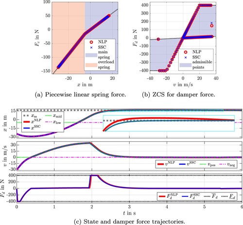
Subsequently, the remaining results of Table 3 are analysed to identify tendencies. As stated in Section 2.2.1, the additional objective terms (55b) represent a relaxation of the constraints comparable with slack variables. Besides serving as feedback for determining convergence, this relaxation provides robustness regarding the initialisation. This is reflected in the results by a successful convergence of the SSC algorithm in 100% of the test cases, even though a rather poor initial guess was used. The accuracy of the computed solutions is evaluated using the mean values of the main cost function (48(48) $\begin{array}{r}{J}_{\mathrm{s}\mathrm{s}}\sum _{i=0}^{n_{\mathrm{s}\mathrm{e}\mathrm{g}}-1}\frac{{\mathrm{\Delta }}_i}{6}\left(e_{\mathrm{s}\mathrm{s},i}^2+4e_{\mathrm{s}\mathrm{s},i+\frac{1}{2}}^2+e_{\mathrm{s}\mathrm{s},i+1}^2\right).\end{array}$(48) ) and of the averaged errors (57(57) $\begin{array}{r}{\overline{e}}_{F_d}\frac{1}{n_{\mathrm{p}\mathrm{t}\mathrm{s}}}\sum _{k\in K}\left|F_{d,k}^{\mathrm{N}\mathrm{L}\mathrm{P}}-F_{d,k}^{\mathrm{S}\mathrm{S}\mathrm{C}}\right|\end{array}$(57) ) and (58(58) $\begin{array}{r}{\overline{e}}_{\mathrm{s}\mathrm{s}}\frac{1}{n_{\mathrm{p}\mathrm{t}\mathrm{s}}}\sum _{k\in K}|x_k-x_{\mathrm{s}\mathrm{s},k}|\end{array}$(58) ) defined as (59) $\begin{array}{r}{\overline{J}}_{\mathrm{s}\mathrm{s}}\sum _{i=1}^{10}{J}_{\mathrm{s}\mathrm{s},i},\overline{{\overline{e}}_{F_d}}\sum _{i=1}^{10}{\overline{e}}_{F_d,i}\mathrm{a}\mathrm{n}\mathrm{d}\overline{{\overline{e}}_{\mathrm{s}\mathrm{s}}}\sum _{i=1}^{10}{\overline{e}}_{\mathrm{s}\mathrm{s},i}.\end{array}$(59) These values represent the respective mean value over all 10 OPs, due to 10 different initial values, for one specified number of collocation segments $n_{\mathrm{s}\mathrm{e}\mathrm{g}}$. With $\overline{{\overline{e}}_{F_d}}\le 3.51\mathrm{N}$ being small compared to the domain of $F_d$, the control trajectories of the SSC approach are close to the trajectories computed by the NLP solver. The small deviation of the mean values in (59(59) $\begin{array}{r}{\overline{J}}_{\mathrm{s}\mathrm{s}}\sum _{i=1}^{10}{J}_{\mathrm{s}\mathrm{s},i},\overline{{\overline{e}}_{F_d}}\sum _{i=1}^{10}{\overline{e}}_{F_d,i}\mathrm{a}\mathrm{n}\mathrm{d}\overline{{\overline{e}}_{\mathrm{s}\mathrm{s}}}\sum _{i=1}^{10}{\overline{e}}_{\mathrm{s}\mathrm{s},i}.\end{array}$(59) ) between the SSC solution and the NLP solution indicates that both algorithms converged to a similar solution. Considering the mean value ${\overline{J}}_{\mathrm{s}\mathrm{s}}$ of the main objective function, the NLP solver yields lower objective values than the SSC algorithm. As previously discussed, the mean deviance $\overline{{\overline{e}}_{\mathrm{s}\mathrm{s}}}$ from the steady-state position is smaller when using the SSC algorithm.

The SSC approach greatly reduces the overall computation time $t_{\mathrm{\Sigma }}^{\mathrm{S}\mathrm{S}\mathrm{C}}$ and requires up to only 18.20% of the computation time needed by the NLP solver. The time advantage of the SSC algorithm over the NLP optimiser will be even bigger for asymmetric zonally convex damper sets. Such asymmetric sets require additional discontinuities in the NLP problem but can be easily implemented within the SSC procedure by using differing parameters for the individual convex subsets. As mentioned in Section 2.4, various aspects influence the runtime of the SSC algorithm which is reflected in the results: With rising number of collocation segments, the mean solution time increases and the computation time of SSC increases less than the NLP solution time. Another mentioned effect on runtime is the quality of the initial guess. The provided guess with zero vectors is of varying quality for the individual initial value conditions. A better initial guess in terms of the correct signs of the state trajectories reduces the number of superordinate iterations and thus the overall computation time. Hence, the sensitivity in regards to the initial guess is elaborated in the following section.

The pure optimisation time $t_{\mathrm{o}\mathrm{p}\mathrm{t},\mathrm{\Sigma }}^{\mathrm{S}\mathrm{S}\mathrm{C}}$ reduces up to 6.45% of the corresponding NLP time and is generally significantly shorter than its overall computation time $t_{\mathrm{\Sigma }}^{\mathrm{S}\mathrm{S}\mathrm{C}}$. Since the projection step of the SSC algorithm employs only simple computations using minimum and maximum functions with linear time complexity, the time spent outside of the QP solver, which solves convex QP-problems in polynomial time, seems quite long. Unfortunately, substantial time losses occur at building the updated optimisation model via JuMP and the Gurobi-wrapper. For future implementations, it is advisable to implement the SSC algorithm via C-code to circumvent this problem and minimise the overall computation time.

3.3. Influence of initial guess on results

In this section, the OPs (51(51a) $\begin{array}{rl}\underset{\mathbf{\text{u}},\mathbf{\text{X}}}{min}& J_{\mathrm{s}\mathrm{s}}\end{array}$(51a) ) and (55(55a) $\begin{array}{rl}\underset{\mathbf{\text{P}}}{min}& J_{\mathrm{s}\mathrm{s}}+\tau \sum _{k\in K}{l}_{\mathrm{a}\mathrm{b}\mathrm{s},x,k}+l_{\mathrm{a}\mathrm{b}\mathrm{s},v,k}\mathrm{w}\mathrm{i}\mathrm{t}\mathrm{h}\end{array}$(55a) ) are modified to consider the nonlinear spring characteristic with three piecewise linear segments depicted in Figure 5b. The NLP problem (51(51a) $\begin{array}{rl}\underset{\mathbf{\text{u}},\mathbf{\text{X}}}{min}& J_{\mathrm{s}\mathrm{s}}\end{array}$(51a) ) is adjusted by replacing the spring force $F_{c,2,k}^{\mathrm{N}\mathrm{L}\mathrm{P}}$ in the differential equation system considered in constraint (51b) by (60) $\begin{array}{rl}{F}_{c,3,k}^{\mathrm{N}\mathrm{L}\mathrm{P}}& ={\mathrm{m}\mathrm{a}\mathrm{x}}_{ϵ}\left[{\mathrm{m}\mathrm{i}\mathrm{n}}_{ϵ}\left(c_{\mathrm{m}\mathrm{i}\mathrm{d}}{x}_k,c_{\mathrm{l}\mathrm{o}\mathrm{w}}{x}_k\right.\right.\\ & \left.\left.-{\underset{\_}{x}}_{\mathrm{t}\mathrm{r}}(c_{\mathrm{l}\mathrm{o}\mathrm{w}}-c_{\mathrm{m}\mathrm{i}\mathrm{d}})\right),c_{\mathrm{u}\mathrm{p}}{x}_k+{\overline{x}}_{\mathrm{t}\mathrm{r}}(c_{\mathrm{m}\mathrm{i}\mathrm{d}}-c_{\mathrm{u}\mathrm{p}})\right]\end{array}$(60) using the smooth maximum function (61) $\begin{array}{r}{\mathrm{m}\mathrm{a}\mathrm{x}}_{ϵ}(x,y)\frac{1}{2}\left((x+y)+\sqrt{(x-y{)}^2+ϵ}\right).\end{array}$(61) The adaptation of the QP problem (55(55a) $\begin{array}{rl}\underset{\mathbf{\text{P}}}{min}& J_{\mathrm{s}\mathrm{s}}+\tau \sum _{k\in K}{l}_{\mathrm{a}\mathrm{b}\mathrm{s},x,k}+l_{\mathrm{a}\mathrm{b}\mathrm{s},v,k}\mathrm{w}\mathrm{i}\mathrm{t}\mathrm{h}\end{array}$(55a) ) requires slightly more changes. The auxiliary decision variables for the position (53c(53c) $\begin{array}{r}\begin{array}{rl}{\mathbf{\text{X}}}_{\mathrm{a}\mathrm{u}\mathrm{x}}& =\left[\begin{array}{cccc}{\mathbf{\text{x}}}_{\mathrm{a}\mathrm{u}\mathrm{x},0}& {\mathbf{\text{x}}}_{\mathrm{a}\mathrm{u}\mathrm{x},0.5}& \dots & {\mathbf{\text{x}}}_{\mathrm{a}\mathrm{u}\mathrm{x},n_{\mathrm{s}\mathrm{e}\mathrm{g}}}\end{array}\right]\in {\mathbb{R}}^{2\times n_{\mathrm{p}\mathrm{t}\mathrm{s}}}\mathrm{w}\mathrm{i}\mathrm{t}\mathrm{h}{\mathbf{\text{x}}}_{\mathrm{a}\mathrm{u}\mathrm{x},k}\left[\begin{array}{c}{x}_{\mathrm{m}\mathrm{i}\mathrm{d},k}\\ x_{\mathrm{l}\mathrm{o}\mathrm{w},k}\end{array}\right]\end{array}\end{array}$(53c) ) are augmented resulting in (62) $\begin{array}{r}{\mathbf{\text{x}}}_{\mathrm{a}\mathrm{u}\mathrm{x},k}{\left[\begin{array}{cccc}{x}_{\overline{\mathrm{l}\mathrm{o}\mathrm{w}},k}& x_{\mathrm{l}\mathrm{o}\mathrm{w},k}& x_{\mathrm{u}\mathrm{p},k}& x_{\mathrm{m}\mathrm{i}\mathrm{d},k}\end{array}\right]}^{\mathrm{T}}.\end{array}$(62) Thus, the position space is bisected into a region below and a region above $x={\underset{\_}{x}}_{\mathrm{t}\mathrm{r}}$, whereas the upper region is again bisected into a region below and above $x={\overline{x}}_{\mathrm{t}\mathrm{r}}$. Compared to (54(54a) $\begin{array}{rl}{\breve{\mathbf{\text{u}}}}_k& =\left[\begin{array}{c}{\breve{u}}_{\mathrm{p}\mathrm{o}\mathrm{s},k}\\ {\breve{u}}_{\mathrm{n}\mathrm{e}\mathrm{g},k}\end{array}\right]=\left[\begin{array}{c}max(u_{\mathrm{n}\mathrm{e}\mathrm{g},k}^{\star }+u_{\mathrm{p}\mathrm{o}\mathrm{s},k}^{\star },0)\\ min(u_{\mathrm{n}\mathrm{e}\mathrm{g},k}^{\star }+u_{\mathrm{p}\mathrm{o}\mathrm{s},k}^{\star },0)\end{array}\right],{\breve{\mathbf{\text{x}}}}_k={\mathbf{\text{x}}}_k^{\star }\end{array}$(54a) ), the update procedure remains unchanged for the decision variables of the inputs, states and auxiliary velocities: (63a) $\begin{array}{r}\begin{array}{rl}& \left[\begin{array}{c}{\breve{u}}_{\mathrm{p}\mathrm{o}\mathrm{s},k}\\ {\breve{u}}_{\mathrm{n}\mathrm{e}\mathrm{g},k}\end{array}\right]=\left[\begin{array}{c}max(u_{\mathrm{n}\mathrm{e}\mathrm{g},k}^{\star }+u_{\mathrm{p}\mathrm{o}\mathrm{s},k}^{\star },0)\\ min(u_{\mathrm{n}\mathrm{e}\mathrm{g},k}^{\star }+u_{\mathrm{p}\mathrm{o}\mathrm{s},k}^{\star },0)\end{array}\right],\\ & {\widehat{\mathbf{\text{x}}}}_k={\mathbf{\text{x}}}_k^{\star },\left[\begin{array}{c}{\breve{v}}_{\mathrm{p}\mathrm{o}\mathrm{s},k}\\ {\breve{v}}_{\mathrm{n}\mathrm{e}\mathrm{g},k}\end{array}\right]=\left[\begin{array}{c}max(v_k^{\star },0)\\ min(v_k^{\star },0)\end{array}\right].\end{array}\end{array}$(63a) However, since the position space is partitioned into three segments, the updating routine changes for the auxiliary position states according to (63b) $\begin{array}{r}\begin{array}{rl}\left[\begin{array}{c}{\breve{x}}_{\overline{\mathrm{l}\mathrm{o}\mathrm{w}},k}\\ {\breve{x}}_{\mathrm{l}\mathrm{o}\mathrm{w},k}\end{array}\right]& =\left[\begin{array}{c}max(x_k^{\star },{\underset{\_}{x}}_{\mathrm{t}\mathrm{r}})\\ min(x_k^{\star },{\underset{\_}{x}}_{\mathrm{t}\mathrm{r}})\end{array}\right],\\ \left[\begin{array}{c}{\breve{x}}_{\mathrm{u}\mathrm{p},k}\\ {\breve{x}}_{\mathrm{m}\mathrm{i}\mathrm{d},k}\end{array}\right]& =\left[\begin{array}{c}max({\breve{x}}_{\overline{\mathrm{l}\mathrm{o}\mathrm{w}},k},{\overline{x}}_{\mathrm{t}\mathrm{r}})\\ min({\breve{x}}_{\overline{\mathrm{l}\mathrm{o}\mathrm{w}},k},{\overline{x}}_{\mathrm{t}\mathrm{r}})\end{array}\right].\end{array}\end{array}$(63b) Furthermore, the correct signs are now given by (63c) $\begin{array}{r}\begin{array}{rl}& {\sigma }_{x_{\mathrm{m}\mathrm{u}},k}=\mathrm{s}\mathrm{i}\mathrm{g}\mathrm{n}({\breve{x}}_{\overline{\mathrm{l}\mathrm{o}\mathrm{w}},k}-{\overline{x}}_{\mathrm{t}\mathrm{r}}),{\sigma }_{x_{\mathrm{l}\mathrm{m}},k}=\mathrm{s}\mathrm{i}\mathrm{g}\mathrm{n}(x_k^{\star }-{\underset{\_}{x}}_{\mathrm{t}\mathrm{r}}),\\ & {\sigma }_{v,k}=\mathrm{s}\mathrm{i}\mathrm{g}\mathrm{n}\left(v_k^{\star }\right).\end{array}\end{array}$(63c) With $i\in I$ and $k\in K$, the convex QP problem is formulated as (64a) $\begin{array}{rl}& \underset{\mathbf{\text{P}}}{min}{J}_{\mathrm{s}\mathrm{s}}+\tau \sum _{k\in K}{l}_{\mathrm{a}\mathrm{b}\mathrm{s},x_{\mathrm{m}\mathrm{u}},k}+l_{\mathrm{a}\mathrm{b}\mathrm{s},x_{\mathrm{l}\mathrm{m}},k}+l_{\mathrm{a}\mathrm{b}\mathrm{s},v,k}\mathrm{w}\mathrm{i}\mathrm{t}\mathrm{h}\end{array}$(64a) (64b) $\begin{array}{rl}& \mathrm{s}.\mathrm{t}.\begin{array}{l}{l}_{\mathrm{a}\mathrm{b}\mathrm{s},x_{\mathrm{m}\mathrm{u}},k}(x_{\mathrm{u}\mathrm{p},k}-x_{\mathrm{m}\mathrm{i}\mathrm{d},k})-{\sigma }_{x_{\mathrm{m}\mathrm{u}},k}(x_{\overline{\mathrm{l}\mathrm{o}\mathrm{w}},k}-{\overline{x}}_{\mathrm{t}\mathrm{r}})\\ l_{\mathrm{a}\mathrm{b}\mathrm{s},x_{\mathrm{l}\mathrm{m}},k}(x_{\overline{\mathrm{l}\mathrm{o}\mathrm{w}},k}-x_{\mathrm{l}\mathrm{o}\mathrm{w},k})-{\sigma }_{x_{\mathrm{l}\mathrm{m}},k}(x_k-{\underset{\_}{x}}_{\mathrm{t}\mathrm{r}})\\ l_{\mathrm{a}\mathrm{b}\mathrm{s},v,k}(v_{\mathrm{p}\mathrm{o}\mathrm{s},k}-v_{\mathrm{n}\mathrm{e}\mathrm{g},k})-{\sigma }_{v,k}{v}_k,\end{array}\end{array}$(64b) (64c) $\begin{array}{r}\begin{array}{rl}& {\mathbf{\text{c}}}_{\mathrm{c}\mathrm{o}\mathrm{l}\mathrm{l},i}\stackrel{\left(5\right)}{=}\mathbf{\text{0}}\mathrm{w}\mathrm{i}\mathrm{t}\mathrm{h}{\mathbf{\text{f}}}_k=\left[\begin{array}{c}{v}_k\\ \frac{1}{m}\left(mg-F_{d,k}^{\mathrm{S}\mathrm{S}\mathrm{C}}-F_{c,3,k}^{\mathrm{S}\mathrm{S}\mathrm{C}}\right)\end{array}\right],\\ & F_{d,k}^{\mathrm{S}\mathrm{S}\mathrm{C}}=u_{\mathrm{n}\mathrm{e}\mathrm{g},k}+u_{\mathrm{p}\mathrm{o}\mathrm{s},k}\text{and}\\ & F_{c,3,k}^{\mathrm{S}\mathrm{S}\mathrm{C}}=c_{\mathrm{u}\mathrm{p}}(x_{\mathrm{u}\mathrm{p},k}-{\overline{x}}_{\mathrm{t}\mathrm{r}})+c_{\mathrm{m}\mathrm{i}\mathrm{d}}{x}_{\mathrm{m}\mathrm{i}\mathrm{d},k}+c_{\mathrm{l}\mathrm{o}\mathrm{w}}(x_{\mathrm{l}\mathrm{o}\mathrm{w},k}-{\underset{\_}{x}}_{\mathrm{t}\mathrm{r}}),\end{array}\end{array}$(64c) (64d) $\begin{array}{r}\begin{array}{rl}& x_k\in X\left[\underset{\_}{x},\overline{x}\right],v_k\in V\left[\underset{\_}{v},\overline{v}\right],\\ & u_{\mathrm{n}\mathrm{e}\mathrm{g},k}\in U_{\mathrm{n}\mathrm{e}\mathrm{g}}\left[{\underset{\_}{F}}_d,0\right],u_{\mathrm{p}\mathrm{o}\mathrm{s},k}\in U_{\mathrm{p}\mathrm{o}\mathrm{s}}\left[0,{\overline{F}}_d\right],\\ & v_{\mathrm{n}\mathrm{e}\mathrm{g},k}\in V_{\mathrm{n}\mathrm{e}\mathrm{g}}\left[\underset{\_}{v},0\right],v_{\mathrm{p}\mathrm{o}\mathrm{s},k}\in V_{\mathrm{p}\mathrm{o}\mathrm{s}}\left[0,\overline{v}\right],\\ & x_{\mathrm{l}\mathrm{o}\mathrm{w},k}\in X_{\mathrm{l}\mathrm{o}\mathrm{w}}\left[\underset{\_}{x},{\underset{\_}{x}}_{\mathrm{t}\mathrm{r}}\right],x_{\overline{\mathrm{l}\mathrm{o}\mathrm{w}},k}\in X_{\overline{\mathrm{l}\mathrm{o}\mathrm{w}}}\left[{\underset{\_}{x}}_{\mathrm{t}\mathrm{r}},\overline{x}\right],\\ & x_{\mathrm{m}\mathrm{i}\mathrm{d},k}\in X_{\mathrm{m}\mathrm{i}\mathrm{d}}\left[{\underset{\_}{x}}_{\mathrm{t}\mathrm{r}},{\overline{x}}_{\mathrm{t}\mathrm{r}}\right],x_{\mathrm{u}\mathrm{p},k}\in X_{\mathrm{u}\mathrm{p}}\left[{\overline{x}}_{\mathrm{t}\mathrm{r}},\overline{x}\right]\end{array}\end{array}$(64d) (64e) $\begin{array}{r}\begin{array}{rl}& {\widehat{\mathbf{\text{h}}}}_{\mathrm{z}\mathrm{c}\mathrm{s},p,k}=\left[\begin{array}{cc}-\overline{d}& 1\\ \underset{\_}{d}& -1\end{array}\right]\left[\begin{array}{c}{v}_{\mathrm{p}\mathrm{o}\mathrm{s},k}\\ u_{\mathrm{p}\mathrm{o}\mathrm{s},k}\end{array}\right]\le \mathbf{\text{0}},\\ & {\widehat{\mathbf{\text{h}}}}_{\mathrm{z}\mathrm{c}\mathrm{s},n,k}=\left[\begin{array}{cc}-\underset{\_}{d}& 1\\ \overline{d}& -1\end{array}\right]\left[\begin{array}{c}{v}_{\mathrm{n}\mathrm{e}\mathrm{g},k}\\ u_{\mathrm{n}\mathrm{e}\mathrm{g},k}\end{array}\right]\le \mathbf{\text{0}},\end{array}\end{array}$(64e) (64f) $\begin{array}{r}\begin{array}{rl}& g_{\mathrm{a}\mathrm{f}\mathrm{f},x_{mu},k}=x_{\mathrm{m}\mathrm{i}\mathrm{d},k}+x_{\mathrm{u}\mathrm{p},k}-(x_{\overline{\mathrm{l}\mathrm{o}\mathrm{w}},k}+{\overline{x}}_{\mathrm{t}\mathrm{r}})=0\\ & g_{\mathrm{a}\mathrm{f}\mathrm{f},x_{lm},k}=x_{\mathrm{l}\mathrm{o}\mathrm{w},k}+x_{\overline{\mathrm{l}\mathrm{o}\mathrm{w}},k}-(x_k+{\underset{\_}{x}}_{\mathrm{t}\mathrm{r}})=0\\ & g_{\mathrm{a}\mathrm{f}\mathrm{f},v,k}=v_{\mathrm{p}\mathrm{o}\mathrm{s},k}+v_{\mathrm{n}\mathrm{e}\mathrm{g},k}-v_k=0,\end{array}\end{array}$(64f) (64g) $\begin{array}{r}\begin{array}{rl}& \underset{={\mathbf{\text{h}}}_{\mathrm{a}\mathrm{b}\mathrm{s},x_{\mathrm{m}\mathrm{u}},k}}{\underbrace{\left[\begin{array}{c}{l}_{\mathrm{a}\mathrm{b}\mathrm{s},x_{\mathrm{m}\mathrm{u}},k}{\mid }_{{\sigma }_{x_{\mathrm{m}\mathrm{u}},k}=+1}\\ l_{\mathrm{a}\mathrm{b}\mathrm{s},x_{\mathrm{m}\mathrm{u}},k}{\mid }_{{\sigma }_{x_{\mathrm{m}\mathrm{u}},k}=-1}\end{array}\right]}}\ge \mathbf{\text{0}},\underset{={\mathbf{\text{h}}}_{\mathrm{a}\mathrm{b}\mathrm{s},x_{\mathrm{l}\mathrm{m}},k}}{\underbrace{\left[\begin{array}{c}{l}_{\mathrm{a}\mathrm{b}\mathrm{s},x_{\mathrm{l}\mathrm{m}},k}{\mid }_{{\sigma }_{x_{\mathrm{l}\mathrm{m}},k}=+1}\\ l_{\mathrm{a}\mathrm{b}\mathrm{s},x_{\mathrm{l}\mathrm{m}},k}{\mid }_{{\sigma }_{x_{\mathrm{l}\mathrm{m}},k}=-1}\end{array}\right]}}\ge \mathbf{\text{0}},\\ & \underset{={\mathbf{\text{h}}}_{\mathrm{a}\mathrm{b}\mathrm{s},v,k}}{\underbrace{\left[\begin{array}{c}{l}_{\mathrm{a}\mathrm{b}\mathrm{s},v,k}{\mid }_{{\sigma }_{v,k}=+1}\\ l_{\mathrm{a}\mathrm{b}\mathrm{s},v,k}{\mid }_{{\sigma }_{v,k}=-1}\end{array}\right]}}\ge \mathbf{\text{0}},\end{array}\end{array}$(64g) (64h) $\begin{array}{rl}& {\mathbf{\text{u}}}_0=\left[\begin{array}{c}max(\underset{\_}{d}{v}_{\mathrm{i}\mathrm{v}},0)\\ min(\underset{\_}{d}{v}_{\mathrm{i}\mathrm{v}},0)\end{array}\right],{\mathbf{\text{x}}}_0={\mathbf{\text{x}}}_{\mathrm{i}\mathrm{v}}.\end{array}$(64h) The termination criterium is computed via (65) $\begin{array}{r}{\overline{l}}_{\mathrm{a}\mathrm{b}\mathrm{s}}={∥\left[\begin{array}{c}{l}_{\mathrm{a}\mathrm{b}\mathrm{s},x_{\mathrm{m}\mathrm{u}},0}\\ l_{\mathrm{a}\mathrm{b}\mathrm{s},x_{\mathrm{l}\mathrm{m}},0}\\ l_{\mathrm{a}\mathrm{b}\mathrm{s},v,0}\end{array}\right],\dots ,\left[\begin{array}{c}{l}_{\mathrm{a}\mathrm{b}\mathrm{s},x_{\mathrm{m}\mathrm{u}},n_{\mathrm{s}\mathrm{e}\mathrm{g}}}\\ l_{\mathrm{a}\mathrm{b}\mathrm{s},x_{\mathrm{l}\mathrm{m}},n_{\mathrm{s}\mathrm{e}\mathrm{g}}}\\ l_{\mathrm{a}\mathrm{b}\mathrm{s},v,n_{\mathrm{s}\mathrm{e}\mathrm{g}}}\end{array}\right]∥}_{\mathrm{m}\mathrm{a}\mathrm{x}}.\end{array}$(65)

In order to analyse the effect of the initialisation on the computed solution, several initial guesses are fed to the SSC algorithm aiming at solving the OP with initial value ${\mathbf{\text{x}}}_{\mathrm{i}\mathrm{v},1}$ considering $n_{\mathrm{s}\mathrm{e}\mathrm{g}}=250$ collocation segments. The maximum number of iterations is increased to $q_{\mathrm{m}\mathrm{a}\mathrm{x}}=25$ to check if poor approximations eventually converge. Using the solution of the NLP optimiser ${\mathbf{\text{u}}}_{\mathrm{o}\mathrm{p}\mathrm{t}}^{\mathrm{N}\mathrm{L}\mathrm{P}}$ and ${\mathbf{\text{X}}}_{\mathrm{o}\mathrm{p}\mathrm{t}}^{\mathrm{N}\mathrm{L}\mathrm{P}}$ as reference, the initial guesses are generated using (66) $\begin{array}{r}\begin{array}{rl}& u_{\mathrm{n}\mathrm{e}\mathrm{g},k}^{\star }=k_{\mathrm{i}\mathrm{n}\mathrm{i}\mathrm{t}}min\left(u_{\mathrm{o}\mathrm{p}\mathrm{t},k}^{\mathrm{N}\mathrm{L}\mathrm{P}},0\right),u_{\mathrm{p}\mathrm{o}\mathrm{s},k}^{\star }=k_{\mathrm{i}\mathrm{n}\mathrm{i}\mathrm{t}}max\left(u_{\mathrm{o}\mathrm{p}\mathrm{t},k}^{\mathrm{N}\mathrm{L}\mathrm{P}},0\right),\\ & {\mathbf{\text{x}}}_k^{\star }=k_{\mathrm{i}\mathrm{n}\mathrm{i}\mathrm{t}}{\mathbf{\text{x}}}_{\mathrm{o}\mathrm{p}\mathrm{t},k}^{\mathrm{N}\mathrm{L}\mathrm{P}}\end{array}\end{array}$(66) with $k_{\mathrm{i}\mathrm{n}\mathrm{i}\mathrm{t}}\in \{0.0,0.5,0.75,0.95,1.0,1.05,10.0\}$ which are fed to the SSC update routine. The computations are compared to the results of the NLP problem which is initialised with the same guesses. The results of the individual optimisations are listed in Table 4. As Figure 8(a,b) indicates for $k_{\mathrm{i}\mathrm{n}\mathrm{i}\mathrm{t}}=0$, all solutions satisfy the prescribed constraints: The spring forces lie on the piecewise linear branches and the damper forces are within the admissible area. Considering the objective value $J_{\mathrm{s}\mathrm{s}}$ and mean error ${\overline{e}}_{\mathrm{s}\mathrm{s}}$ in Table 4, the NLP solver converges to the same solution independently which initial guess is supplied. Thus, it is assumed that the computed NLP solution represents the global optimum or is at least very close to it. However, initialisation can have a massive impact on the computation time. Generally, the guesses close to the solution result in shorter computation times. It is striking that both algorithms have the most difficulty converging for $k_{\mathrm{i}\mathrm{n}\mathrm{i}\mathrm{t}}=0.5$ which is not the guess with the biggest difference to the optimal solution. The SSC algorithm converges significantly faster than the NLP solver for all initial guesses. The number of superordinate iterations required by the SSC algorithm is small for good initial guesses. As for $k_{\mathrm{i}\mathrm{n}\mathrm{i}\mathrm{t}}=0.5$, a high number of superordinate iterations can still yield a faster convergence compared to the NLP solver. As already mentioned, the SSC algorithm represents a local method and does not necessarily provide the global optimum, which is reflected in the results. Considering the objective value $J_{\mathrm{s}\mathrm{s}}$ and mean error ${\overline{e}}_{\mathrm{s}\mathrm{s}}$, only the SSC solutions for $k_{\mathrm{i}\mathrm{n}\mathrm{i}\mathrm{t}}\ge 0.5$ are roughly in the vicinity of the global solution. The mean deviance between the input trajectories ${\overline{e}}_{F_d}$ is then rather small. Even though the SSC solutions may not represent the global optimum, the solutions satisfy the prescribed constraints since $q<q_{\mathrm{m}\mathrm{a}\mathrm{x}}$. Thus, they represent a local solution of the piecewise linear problem, which corresponds to the original problem for the example at hand. The results for $k_{\mathrm{i}\mathrm{n}\mathrm{i}\mathrm{t}}=\{0.95,1.0,1.05\}$ confirm that the SSC algorithm converges to the global optimum if the initial guess is in a close vicinity of it.

Figure 8. Optimisation results for SMO application with three-segmented nonlinear spring for $k_{\mathrm{i}\mathrm{n}\mathrm{i}\mathrm{t}}=0$. (a) Piecewise linear spring force with three segments. (b) ZCS for damper force.

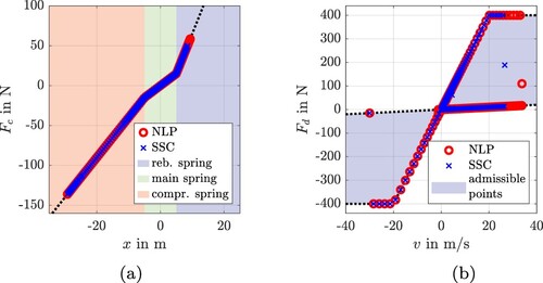
Table 4. Analysis of sensitivity regarding initial guess.

	method		results
$k_{\mathrm{i}\mathrm{n}\mathrm{i}\mathrm{t}}[-]$	NLP	SSC	$J_{\mathrm{s}\mathrm{s}}\left[{\mathrm{m}}^2\mathrm{s}\right]$	${\overline{e}}_{\mathrm{s}\mathrm{s}}\left[\mathrm{m}\right]$	${\overline{e}}_{F_d}\left[\mathrm{N}\right]$	$q[-]$	$t_{\mathrm{o}\mathrm{p}\mathrm{t},\mathrm{\Sigma }}\left[\mathrm{s}\right]$	$t_{\mathrm{\Sigma }}\left[\mathrm{s}\right]$
0.0	✓		1603.95	5.47	–	1	4.589	4.589
0.0		✓	2118.49	9.91	46.63	7	0.493 (10.74%)	0.798 (17.38%)
0.5	✓		1603.95	5.47	–	1	6.347	6.347
0.5		✓	1635.20	5.93	14.43	19	1.450 (22.85%)	2.136 (33.65%)
0.75	✓		1603.95	5.47	–	1	0.557	0.557
0.75		✓	1612.62	5.67	15.77	2	0.179 (32.14%)	0.324 (58.26%)
0.95	✓		1603.95	5.47	–	1	0.473	0.473
0.95		✓	1603.95	5.47	0.01	1	0.075 (15.86%)	0.199 (42.02%)
1.0	✓		1603.95	5.47	–	1	0.417	0.417
1.0		✓	1603.95	5.47	0.01	1	0.072 (17.28%)	0.191 (45.79%)
1.05	✓		1603.95	5.47	–	1	0.427	0.427
1.05		✓	1603.96	5.47	0.20	1	0.084 (19.67%)	0.202 (47.37%)
10.0	✓		1603.95	5.47	–	1	0.981	0.981
10.0		✓	1610.74	5.72	6.71	2	0.149 (15.19%)	0.306 (31.22%)

$k_{\mathrm{i}\mathrm{n}\mathrm{i}\mathrm{t}}$: perturbation parameter for initialisation error; NLP: IPOPT solving NLP problem; SSC: SSC Algorithm 1 with QP problem (64a(64a) $\begin{array}{rl}& \underset{\mathbf{\text{P}}}{min}{J}_{\mathrm{s}\mathrm{s}}+\tau \sum _{k\in K}{l}_{\mathrm{a}\mathrm{b}\mathrm{s},x_{\mathrm{m}\mathrm{u}},k}+l_{\mathrm{a}\mathrm{b}\mathrm{s},x_{\mathrm{l}\mathrm{m}},k}+l_{\mathrm{a}\mathrm{b}\mathrm{s},v,k}\mathrm{w}\mathrm{i}\mathrm{t}\mathrm{h}\end{array}$(64a) ); $J_{\mathrm{s}\mathrm{s}}$: main objective (48(48) $\begin{array}{r}{J}_{\mathrm{s}\mathrm{s}}\sum _{i=0}^{n_{\mathrm{s}\mathrm{e}\mathrm{g}}-1}\frac{{\mathrm{\Delta }}_i}{6}\left(e_{\mathrm{s}\mathrm{s},i}^2+4e_{\mathrm{s}\mathrm{s},i+\frac{1}{2}}^2+e_{\mathrm{s}\mathrm{s},i+1}^2\right).\end{array}$(48) ); ${\overline{e}}_{\mathrm{s}\mathrm{s}}$/${\overline{e}}_{F_d}$: error metrics (58(58) $\begin{array}{r}{\overline{e}}_{\mathrm{s}\mathrm{s}}\frac{1}{n_{\mathrm{p}\mathrm{t}\mathrm{s}}}\sum _{k\in K}|x_k-x_{\mathrm{s}\mathrm{s},k}|\end{array}$(58) ) and (57(57) $\begin{array}{r}{\overline{e}}_{F_d}\frac{1}{n_{\mathrm{p}\mathrm{t}\mathrm{s}}}\sum _{k\in K}\left|F_{d,k}^{\mathrm{N}\mathrm{L}\mathrm{P}}-F_{d,k}^{\mathrm{S}\mathrm{S}\mathrm{C}}\right|\end{array}$(57) ); q: # of superordinate iterations; $t_{\mathrm{o}\mathrm{p}\mathrm{t},\mathrm{\Sigma }}$: cumulative time spent in NLP/QP solver; $t_{\mathrm{\Sigma }}$: total computation time.

As mentioned in Section 2.4, increasing the number of space divisions to depict the three-segmented spring raises computation time. This can be confirmed by comparing solution times of the SSC algorithm for $k_{\mathrm{i}\mathrm{n}\mathrm{i}\mathrm{t}}=0.0$: For the two-segmented spring $t_{\mathrm{o}\mathrm{p}\mathrm{t},\mathrm{\Sigma }}^{\mathrm{S}\mathrm{S}\mathrm{C}}=0.262\mathrm{s}$, $t_{\mathrm{\Sigma }}^{\mathrm{S}\mathrm{S}\mathrm{C}}=0.329\mathrm{s}$ and $q=4$ holds whereas $t_{\mathrm{o}\mathrm{p}\mathrm{t},\mathrm{\Sigma }}^{\mathrm{S}\mathrm{S}\mathrm{C}}=0.493\mathrm{s}$, $t_{\mathrm{\Sigma }}^{\mathrm{S}\mathrm{S}\mathrm{C}}=0.798\mathrm{s}$ and $q=7$ holds for the spring with three segments. Thus, more iterations are required and the average computation time per iteration is increased by 7.52% and 38.6% for $t_{\mathrm{o}\mathrm{p}\mathrm{t},\mathrm{\Sigma }}^{\mathrm{S}\mathrm{S}\mathrm{C}}$ and $t_{\mathrm{\Sigma }}^{\mathrm{S}\mathrm{S}\mathrm{C}}$, respectively. This highlights the importance of an implementation in C-Code to reduce the time required for the updating routine and therefore the overall computation time.

3.4. Rotated space splitting

As elaborated in Section 2.3.1, some sets require to be split using a rotated straight line. Without going into detail, the approach is applied to the example of a hanging SMO with fully linear spring presented in Section 3.1. The OP is parametrised with initial value ${\mathbf{\text{x}}}_{\mathrm{i}\mathrm{v},1}$ and $n_{\mathrm{s}\mathrm{e}\mathrm{g}}=250$ collocation segments. The damper set is rotated by $\phi =7^{\circ }$ resulting in the set depicted in Figure 9(a). This is implemented by applying the changes (36(36a) $\begin{array}{r}\begin{array}{rl}{g}_{\mathrm{a}\mathrm{f}\mathrm{f}}& =({\mathcal{v}}_p+{\mathcal{v}}_n)-\tilde{\mathcal{v}}=0\text{with}\\ \tilde{\mathcal{v}}& ={\mathrm{c}}_{\phi }(v-v_{\mathrm{t}\mathrm{r}})+{\mathrm{s}}_{\phi }({\mathrm{s}}_{\phi }({\mathcal{v}}_p+{\mathcal{v}}_n)+{\mathrm{c}}_{\phi }({\mathcal{u}}_p+{\mathcal{u}}_n))\end{array}\end{array}$(36a) ) to the convex QP problem with fully linear spring. As depicted in Figure 9(a), the SSC algorithm computes damper forces which all lie within the admissible area. Although this example represents an artificial use-case, the corresponding position trajectories in Figure 9(b) prove that the rotated set yields a reduction of the objective. Starting with $x_{\mathrm{i}\mathrm{v},1}<x_{\mathrm{s}\mathrm{s}}$ in a compression phase with $v_{\mathrm{i}\mathrm{v},1}<0$, the mass is first decelerated and then accelerated using $F_d<0$ at v>0, hence active forces. These active forces enable a faster attainment of the steady-state position. Due to the similarity to the previous examples, no further discussion is given.

4. Conclusions

This article has presented a novel local solution method for efficiently solving nonconvex optimal control problems. Splitting the space of inputs and states enables the formulation of QP subproblems which are solved iteratively. The method is capable of considering two types of nonconvexities: ZCSs and equality constraints with possibly multiple univariate nonlinearities. The approach decomposes the nonconvexities into affine parts which are linked appropriately to approximate the original problem with scalable approximation error. It has been shown that the SSC algorithm converges to a local optimum of this approximated problem. The quality of the solution depends on the initial guess. For good initial guesses, the method converges to solutions close to the global one. A comparison of this successive convexification technique with other existing methods has been given, highlighting the advantages SSC provides.

Figure 9. SSC optimisation results for SMO application with fully linear spring and rotated damper set. (a) Rotated ZCS for damper force. (b) Position trajectory; $x^{\mathrm{S}\mathrm{S}\mathrm{C}}$: original damper force set; $x^{\mathrm{S}\mathrm{S}\mathrm{C},\phi }$: rotated damper force set.

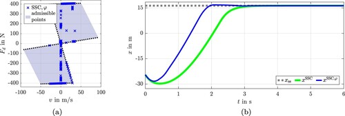
Subsequently, possible directions for future research are disclosed. Even though it would not change the algorithm, using nondifferentiable constraint qualifications (Ye, 2004) could potentially avoid the AVC-smoothing required for continuous differentiability regarding the convergence proof. Due to the low computation time and robust convergence, the SSC method seems to be a promising approach for real-time optimal control applications. In this context, using MPC could provide sufficiently good initial guesses (Diehl et al., 2005; Gros et al., 2020) resulting in good SSC solutions. In order to enhance applicability, the SSC approach could be combined with other iterative linearisation schemes like (Carvalho et al., 2013; Liniger et al., 2015; Mao et al., 2017; Simon et al., 2013) which could enable considering collision avoidance constraints. Furthermore, extending the SSC approach to bivariate nonlinearities in equality constraints would enlarge the possible scope of applications. Moreover, applying a more sophisticated updating procedure for the penalty parameter would improve computation times (Maratos, 1978; Mayne & Maratos, 1979; Nocedal & Wright, 2006). For applications with real-time capability requirement, it is recommended to implement the algorithm via tailored C-code to avoid the overhead introduced by the high-level routines of JuMP and the Gurobi-wrapper. Then, the required time for the updating step can be greatly reduced to linear time complexity resulting in shorter overall computation times.

Notation

$\widehat{(\cdot )}$	=	Transformed constraints depending on $\mathbf{\text{z}}$
$\breve{(\cdot )}$	=	Projected initial solution of $(\cdot )$
$(\cdot {)}^{\star }$	=	Previous optimal solution of $(\cdot )$
$(\cdot {)}_{\mathrm{t}\mathrm{r}}$	=	Transition point for space bisection
$\underset{\_}{(\cdot )},\overline{(\cdot )}$	=	Lower and upper bound of $(\cdot )$
$(\cdot {)}_{n/\mathrm{n}\mathrm{e}\mathrm{g}}$	=	Negative region of bisected space
$(\cdot {)}_{p/\mathrm{p}\mathrm{o}\mathrm{s}}$	=	Positive region of bisected space
$\alpha (\cdot )$	=	Smoothable absolute value function
$\widehat{\mathbf{\text{A}}},\widehat{\mathbf{\text{b}}}$	=	Matrix and vector of affine transformation function
$\mathbf{\text{A}},\mathbf{\text{B}},\mathbf{\text{k}}$	=	Matrices and vector for system behaviour description
${\mathbf{\text{A}}}_{\mathrm{z}\mathrm{c}\mathrm{s}},{\mathbf{\text{b}}}_{\mathrm{z}\mathrm{c}\mathrm{s}}$	=	Matrix and vector describing affine ZCSs
$c_{(\cdot )}$	=	Spring stiffness of corresponding segment $(\cdot )$ for SMO
$\mathbf{\text{c}}$	=	Left-hand sides of equality constraints
$\widetilde{\mathbf{\text{c}}}$	=	Left-hand sides of continuous-time equality constraints
${\mathbf{\text{c}}}_{\mathrm{c}\mathrm{o}\mathrm{l}\mathrm{l}}$	=	Left-hand sides of collocation equality constraints
${\mathbf{\text{c}}}_{\mathrm{t}\mathrm{o}\mathrm{t}}$	=	Left-hand sides of aggregated equality constraints
d	=	Damper coefficient for SMO
${\mathrm{\Delta }}_i$	=	Width of $i^{\mathrm{t}\mathrm{h}}$ collocation segment
${\overline{e}}_{F_d}$	=	Mean absolute deviance in damper force trajectories between NLP and SSC solution
$e_{\mathrm{s}\mathrm{s}}$	=	Steady-state position deviation of SMO
${\overline{e}}_{\mathrm{s}\mathrm{s}}$	=	Mean absolute deviance between position trajectory and steady-state position
${ϵ}_g$	=	Error tolerance for linearised AVCs
${ϵ}_s$	=	Smoothing parameter for absolute value function
${\mathbf{\text{E}}}_{\mathrm{\Sigma }/\mathrm{\Delta }/z}$	=	Matrices for selecting specific decision variables
$\mathbf{\text{f}}$	=	Right-hand side of differential equation system of model
${\mathbf{\text{f}}}_{\mathrm{\Phi }}$	=	Affine approximation of right-hand side of model equations
${\mathbf{\text{f}}}_{\mathrm{p}\mathrm{w}\mathrm{l}}$	=	Composition of univariate nonlinearities approximable by piecewise linear curves
$F_c$	=	Spring force of SMO
$F_d$	=	Damper force of SMO
ϕ	=	Intermediate objective term
${\mathbf{\Phi }}_{x/u/\mathrm{p}\mathrm{w}\mathrm{l}}$	=	Mapping functions affine in the decision variables
g	=	Gravitational acceleration for SMO
${\mathbf{\text{g}}}_{\mathrm{a}\mathrm{b}\mathrm{s}}$	=	Left-hand sides of AVCs for space splitting
${\mathbf{\text{g}}}_{\mathrm{a}\mathrm{f}\mathrm{f}}$	=	Left-hand sides of affine constraints for space splitting
$\mathbf{\text{h}}$	=	Left-hand sides of inequality constraints
$\widetilde{\mathbf{\text{h}}}$	=	Left-hand sides of continuous-time inequality constraints
${\mathbf{\text{h}}}_{\mathrm{a}\mathrm{b}\mathrm{s}}$	=	Left-hand sides of relaxed (inequality) AVCs for space splitting
${\mathbf{\text{h}}}_{\mathrm{t}\mathrm{o}\mathrm{t}}$	=	Left-hand sides of aggregated inequality constraints
${\mathbf{\text{h}}}_{\mathrm{z}\mathrm{c}\mathrm{s}}$	=	Left-hand sides of ZCS inequality constraints
$I$	=	Set of collocation segment indices
J	=	Objective function
$\tilde{J}$	=	Continuous-time objective functional
$J_{\mathrm{s}\mathrm{s}}$	=	Objective function for steady-state position deviation of SMO
$k_{\mathrm{i}\mathrm{n}\mathrm{i}\mathrm{t}}$	=	Perturbation parameter for initialisation error
$K$	=	Set of collocation point indices
${\mathbf{\text{l}}}_{\mathrm{a}\mathrm{b}\mathrm{s}}$	=	Left-hand sides of linearised AVCs for space splitting
m	=	Mass of SMO
$n_c$	=	Number of equality constraints
$n_h$	=	Number of inequality constraints
$n_{\mathrm{p}\mathrm{t}\mathrm{s}}$	=	Number of collocation points
$n_s$	=	Number of auxiliary decision variables
$n_{\mathrm{s}\mathrm{e}\mathrm{g}}$	=	Number of collocation segments
$n_u$	=	Number of input decision variables
$n_w$	=	Number of original decision variables
$n_x$	=	Number of state decision variables
$O(\cdot )$	=	Landau-notation for computational complexity
${\mathbf{\text{P}}}_0,{\mathbf{\text{q}}}_0,r_0$	=	parameters of quadratic objective
q	=	Number of superordinate iterations in SSC algorithm
$q_{\mathrm{m}\mathrm{a}\mathrm{x}}$	=	Maximum number of superordinate iterations
${\mathbb{R}}^n$	=	Set of n-dimensional, real vectors
$s_w$	=	Slack variable for AVC
$S_{(\cdot )}$	=	Set described by inequality constraints
${\sigma }_{(\cdot )}$	=	Sign of corresponding AVC
$\mathbf{\Sigma }$	=	Matrix containing all linearisation points of AVCs
t	=	Time
$t_{\mathrm{o}\mathrm{p}\mathrm{t},\mathrm{\Sigma }}$	=	Cumulative time spent in solver
$t_{\mathrm{\Sigma }}$	=	Total computation time
τ	=	Penalty parameter for additional objective terms
$\vartheta$	=	Terminal objective term
$\mathbf{\text{u}}$	=	Input vector of system
$U$	=	Bounding-box set for system inputs
${\mathbf{\text{U}}}_0^{\star }$	=	Initial solution for input decision variables
v	=	Deflection velocity of SMO
$\mathbf{\text{w}}$	=	Vector of original decision variables
${\mathbf{\text{w}}}_{\mathrm{a}\mathrm{u}\mathrm{x}}$	=	Vector of auxiliary decision variables
$w_{\mathrm{l}\mathrm{o}\mathrm{w}/\mathrm{u}\mathrm{p}}$	=	Lower/upper region of bisected space of w
x	=	Deflection position of SMO
$x_{\mathrm{s}\mathrm{s}}$	=	Steady-state position of SMO
$x_{\mathrm{l}\mathrm{o}\mathrm{w}/\overline{\mathrm{l}\mathrm{o}\mathrm{w}}}$	=	Lower/upper region of position space bisection for SMO
$x_{\mathrm{m}\mathrm{i}\mathrm{d}/\mathrm{u}\mathrm{p}}$	=	Lower/upper region of bisected position space $x_{\overline{\mathrm{l}\mathrm{o}\mathrm{w}}}$ for SMO
$\mathbf{\text{x}}$	=	State vector of system
$X$	=	Bounding-box set for system states
${\mathbf{\text{X}}}_0^{\star }$	=	Initial solution for state decision variables
${\mathbf{\text{x}}}_{\mathrm{i}\mathrm{v}}$	=	Initial value of system state for SMO
$\mathbf{\text{z}}$	=	Vector of accumulated decision variables
$\widetilde{\mathbf{\text{z}}}$	=	Argument vector for absolute value function
${\widetilde{\mathbf{\text{z}}}}^{\star }$	=	Linearisation point for AVCs

Disclosure statement

No potential conflict of interest was reported by the author(s).

References

- Acikmese, B., & Blackmore, L. (2011). Lossless convexification of a class of optimal control problems with non-convex control constraints. Automatica, 47(2), 341–347. https://doi.org/10.1016/j.automatica.2010.10.037
- Acikmese, B., & Ploen, S. R. (2007). Convex programming approach to powered descent guidance for Mars landing. Journal of Guidance, Control, and Dynamics, 30(5), 1353–1366. https://doi.org/10.2514/1.27553
- Armaou, A., & Ataei, A. (2014). Piece-wise constant predictive feedback control of nonlinear systems. Journal of Process Control, 24(4), 326–335. https://doi.org/10.1016/j.jprocont.2014.02.002
- Betts, J. T. (2010). Practical methods for optimal control and estimation using nonlinear programming (2nd ed.). Society for Industrial and Applied Mathematics.
- Boyd, S., & Vandenberghe, L. (2004). Convex optimization (7th ed.). Cambridge University Press.
- Carvalho, A., Gao, Y., Gray, A., Tseng, H. E., & Borrelli, F. (2013). Predictive control of an autonomous ground vehicle using an iterative linearization approach. 16th International IEEE Conference on Intelligent Transportation Systems (ITSC 2013) (p. 2335–2340). doi:10.1109/ITSC.2013.6728576
- Chen, J., Zhan, W., & Tomizuka, M. (2017). Constrained iterative LQR for on-road autonomous driving motion planning. 2017 IEEE 20th International Conference on Intelligent Transportation Systems (ITSC) (p. 1–7). doi:10.1109/ITSC.2017.8317745
- Cibulka, V., Hanis, T., & Hromcik, M. (2019). Data-driven identification of vehicle dynamics using Koopman operator. https://arxiv.org/abs/1903.06103
- Cibulka, V., Haniš, T., Korda, M., & Hromčík, M. (2020). Model predictive control of a vehicle using Koopman operator. IFAC-PapersOnLine, 53(2), 4228–4233. https://doi.org/10.1016/j.ifacol.2020.12.2469(21st IFAC World Congress)
- d'Aspremont, A., & Boyd, S. (2003). Relaxations and randomized methods for nonconvex QCQPs. Retrieved November 24, Retrieved 2020, from https://web.stanford.edu/class/ee392o/relaxations.pdf.
- Del Re, L., Chapuis, J., & Nevistic, V. (1993). Predictive control with embedded feedback linearization for bilinear plants with input constraints. Proceedings of 32nd IEEE Conference on Decision and Control (Vol. 4, p. 2984–2989). doi:10.1109/CDC.1993.325747
- Diehl, M., Bock, H. G., & Schlöder, J. P. (2005). A real-time iteration scheme for nonlinear optimization in optimal feedback control. SIAM Journal on Control and Optimization, 43(5), 1714–1736. https://doi.org/10.1137/S0363012902400713
- Di Pillo, G., & Grippo, L. (1989). Exact penalty functions in constrained optimization. SIAM Journal on Control and Optimization, 27(6), 1333–1360. https://doi.org/10.1137/0327068
- Dunning, I., Huchette, J., & Lubin, M. (2017). JuMP: A modeling language for mathematical optimization. SIAM Review, 59(2), 295–320. https://doi.org/10.1137/15M1020575
- Falcone, P., Borrelli, F., Asgari, J., Tseng, H. E., & Hrovat, D. (2007). Predictive active steering control for autonomous vehicle systems. IEEE Transactions on Control Systems Technology, 15(3), 566–580. https://doi.org/10.1109/TCST.2007.894653
- Fang, Y., & Armaou, A. (2015). Nonlinear model predictive control using a bilinear Carleman linearization-based formulation for chemical processes. 2015 American Control Conference (ACC) (p. 5629–5634). doi:10.1109/ACC.2015.7172221
- Ferreau, H., Almér, S., Verschueren, R., Diehl, M., Frick, D., Domahidi, A., Jerez, J.L., Stathopoulos, G., & Jones, C. (2017). Embedded optimization methods for industrial automatic control. IFAC-PapersOnLine, 50(1), 13194–13209. https://doi.org/10.1016/j.ifacol.2017.08.1946
- Gros, S., Zanon, M., Quirynen, R., Bemporad, A., & Diehl, M. (2020). From linear to nonlinear MPC: Bridging the gap via the real-time iteration. International Journal of Control, 93(1), 62–80. https://doi.org/10.1080/00207179.2016.1222553
- Gurobi Optimization (2020). Gurobi optimizer reference manual. Retrieved November 24, 2020, from https://www.gurobi.com/wp-content/plugins/hd_documentations/documentation/9.1/refman.pdf.
- Han, S. P., & Mangasarian, O. L. (1979). Exact penalty functions in nonlinear programming. Mathematical programming, 17(1), 251–269. https://doi.org/10.1007/BF01588250
- Karmarkar, N. (1984). A new polynomial-time algorithm for linear programming. Combinatorica, 4, 373–395. https://doi.org/10.1007/BF02579150
- Kelly, M. (2017). An introduction to trajectory optimization: How to do your own direct collocation. SIAM Review, 59(4), 849–904. https://doi.org/10.1137/16M1062569
- Khalil, H. K. (2002). Nonlinear systems (3rd ed.). Prentice Hall.
- Korda, M., & Mezić, I. (2018). Linear predictors for nonlinear dynamical systems: Koopman operator meets model predictive control. Automatica, 93(1), 149–160. https://doi.org/10.1016/j.automatica.2018.03.046
- Kozlov, M., Tarasov, S., & Khachiyan, L. (1980). The polynomial solvability of convex quadratic programming. USSR Computational Mathematics and Mathematical Physics, 20(5), 223–228. https://doi.org/10.1016/0041-5553(80)90098-1
- Kurtz, M. J., & Henson, M. A. (1997). Input-output linearizing control of constrained nonlinear processes. Journal of Process Control, 7(1), 3–17. https://doi.org/10.1016/S0959-1524(96)00006-6
- Liberti, L. (2008). Introduction to global optimization. Retrieved January 23, 2021, from https://www.lix.polytechnique.fr/liberti/teaching/globalopt-lima.pdf.
- Liberti, L., & Maculan, N. (2006). Global optimization – from theory to implementation. Springer Science and Business Media.
- Liniger, A., Domahidi, A., & Morari, M. (2015). Optimization-based autonomous racing of 1:43 scale RC cars. Optimal Control Applications and Methods, 36, 628–647. https://doi.org/10.1002/oca.2123
- Lipp, T., & Boyd, S. (2016). Variations and extension of the convex–concave procedure. Optimization and Engineering, 17, 263–287. https://doi.org/10.1007/s11081-015-9294-x
- Mangasarian, O. L. (2015). A hybrid algorithm for solving the absolute value equation. Optimization Letters, 9, 1469–1474. https://doi.org/10.1007/s11590-015-0893-4
- Mao, Y., Dueri, D., Szmuk, M., & Açíkmeşe, B. (2017). Successive Convexification of Non-Convex Optimal Control Problems with State Constraints. IFAC-PapersOnLine, 50(1), 4063–4069. https://doi.org/10.1016/j.ifacol.2017.08.789(20th IFAC World Congress)
- Mao, Y., Szmuk, M., & Açíkmeşe, B. (2016). Successive convexification of non-convex optimal control problems and its convergence properties. 2016 IEEE 55th Conference on Decision and Control (CDC) (p. 3636–3641). https://doi.org/10.1109/CDC.2016.7798816
- Maratos, N. (1978). Exact penalty function algorithms for finite dimensional and control optimization problems [Unpublished doctoral dissertation]. Imperial College London (University of London).
- Mayne, D. Q. (1973). Differential dynamic programming – A unified approach to the optimization of dynamic systems. In C. Leondes (Ed.), Control and dynamic systems (Vol. 10, p. 179–254). Academic Press.
- Mayne, D. Q., & Maratos, N. (1979). A first order, exact penalty function algorithm for equality constrained optimization problems. Mathematical Programming, 16(1), 303–324. https://doi.org/10.1007/BF01582118
- Mollov, S., Babuska, R., Abonyi, J., & Verbruggen, H. B. (2004). Effective optimization for fuzzy model predictive control. IEEE Transactions on Fuzzy Systems, 12(5), 661–675. https://doi.org/10.1109/TFUZZ.2004.834812
- Mollov, S., Babuška, R., Roubos, J., & Verbruggen, H. (1998). MIMO predictive control by multiple-step linearization of Takagi-Sugeno fuzzy models. IFAC Proceedings Volumes, 31(29), 197–202. https://doi.org/10.1016/S1474-6670(17)38944-9(7th IFAC Symposium on Artificial Intelligence in Real Time Control 1998., Grand Canyon National Park, USA, 5–8 October)
- Nocedal, J., & Wright, S. (2006). Numerical optimization. Springer Science and Business Media.
- Park, J., & Boyd, S. (2017). General heuristics for nonconvex quadratically constrained quadratic programming. https://arxiv.org/abs/1703.07870
- Perantoni, G., & Limebeer, D. J. (2014). Optimal control for a Formula One car with variable parameters. Vehicle System Dynamics, 52(5), 653–678. https://doi.org/10.1080/00423114.2014.889315
- Raković, S. V., & Levine, W. S. (2018). Handbook of model predictive control. Springer.
- Ryoo, H., & Sahinidis, N. (1995). Global optimization of nonconvex NLPs and MINLPs with applications in process design. Computers and Chemical Engineering, 19(5), 551–566. https://doi.org/10.1016/0098-1354(94)00097-2
- Savaresi, S. M., Poussot-Vassal, C., Spelta, C., Sename, O., & Dugard, L. (2010). Semi-active suspension control design for vehicles (1st ed.). Elsevier.
- Schnelle, F., & Eberhard, P. (2015). Constraint mapping in a feedback linearization/MPC scheme for trajectory tracking of underactuated multibody systems. IFAC-PapersOnLine, 48(23), 446–451. https://doi.org/10.1016/j.ifacol.2015.11.319(5th IFAC Conference on Nonlinear Model Predictive Control NMPC 2015)
- Sedlacek, T., Odenthal, D., & Wollherr, D. (2020a). Convexification of semi-activity constraints applied to minimum-time optimal control for vehicles with semi-active limited-slip differential. In 17th International Conference on Informatics in Control, Automation and Robotics – volume 1: Icinco (p. 15–25). SciTePress.
- Sedlacek, T., Odenthal, D., & Wollherr, D. (2020b). Minimum-time optimal control for battery electric vehicles with four wheel-independent drives considering electrical overloading. Vehicle System Dynamics, 1–25. https://doi.org/10.1080/00423114.2020.1823004
- Sedlacek, T., Odenthal, D., & Wollherr, D. (2020c). Minimum-time optimal control for vehicles with active rear-axle steering, transfer case and variable parameters. Vehicle System Dynamics, 59(8), 1227–1255. https://doi.org/10.1080/00423114.2020.1742925
- Seki, H., Ooyama, S., & Ogawa, M. (2004). Nonlinear model predictive control using successive linearization. Transactions of the Society of Instrument and Control Engineers, E-3(1), 66–72. https://www.sice.jp/e-trans/papers/E3-9.pdf
- Simon, D., Löfberg, J., & Glad, T. (2013). Nonlinear model predictive control using feedback linearization and local inner convex constraint approximations. 2013 European Control Conference (ECC) (p. 2056–2061). https://doi.org/10.23919/ECC.2013.6669575
- Tanaka, K., & Wang, H. O. (2004). Fuzzy control systems design and analysis – a linear matrix inequality approach. John Wiley and Sons.
- Tassa, Y., Erez, T., & Todorov, E. (2012). Synthesis and stabilization of complex behaviors through online trajectory optimization. 2012 IEEE/RSJ International Conference on Intelligent Robots and Systems (p. 4906–4913). https://doi.org/10.1109/IROS.2012.6386025
- Tassa, Y., Mansard, N., & Todorov, E. (2014). Control-limited differential dynamic programming. 2014 IEEE International Conference on Robotics and Automation (ICRA) (p. 1168–1175). https://doi.org/10.1109/ICRA.2014.6907001
- Tawarmalani, M., & Sahinidis, N. V. (2002). Convexification and global optimization in continuous and mixed-integer nonlinear programming - theory, algorithms, software, and applications. Springer Science and Business Media.
- Verschueren, R. (2018). Convex approximation methods for nonlinear model predictive control [Unpublished doctoral dissertation]. University of Freiburg.
- Wächter, A., & Biegler, L. T. (2006). On the implementation of an interior-point filter line-search algorithm for large-scale nonlinear programming. Mathematical Programming, 106(1), 25–57. https://doi.org/10.1007/s10107-004-0559-y
- Xie, Z., Liu, C. K., & Hauser, K. (2017). Differential dynamic programming with nonlinear constraints. 2017 IEEE International Conference on Robotics and Automation (ICRA) (p. 695–702). https://doi.org/10.1109/ICRA.2017.7989086
- Ye, J. J. (2004). Nondifferentiable multiplier rules for optimization and Bilevel optimization problems. SIAM Journal on Optimization, 15(1), 252–274. https://doi.org/10.1137/S1052623403424193
- Zorich, V. A. (2016). Mathematical analysis I. Springer.