Efficiency-aware nonlinear model-predictive control with real-time iteration scheme for wave energy converters

ABSTRACT

Several solutions have been proposed in the literature to maximise the harvested ocean energy, but only a few consider the overall efficiency of the power take-off system. The fundamental problem of incorporating the power take-off system efficiency is that it leads to a nonlinear and non-convex optimal control problem. The main disadvantage of the available solutions is that none solve the optimal control problem in real-time. This paper presents a nonlinear model predictive control (NMPC) approach based on the real-time iteration (RTI) scheme to incorporate the power take-off system's efficiency when solving the optimal control problem at each time step in a control law aimed at maximising the energy extracted. The second contribution of this paper is the derivation of a condensing algorithm $O(N^2)$ for ‘output-only’ cost functions required to improve computational efficiency. Finally, the RTI-NMPC approach is tested using a scaled model of the Wavestar design, demonstrating the benefit of this new control formulation.

KEYWORDS:

• Wave energy converters
• nonlinear model predictive controller
• real-time iteration
• power take-off-system efficiency
• condensing algorithm $O(N^2)$

1. Introduction

One of several challenges that wave energy technologies confront is their inability to produce electricity at a cost comparable with other grid-scale generation technologies like natural gas and wind (Coe et al., 2021, may). Several studies have identified the refining of advanced control strategies as a way to improve energy capture efficiency significantly and, as a result, give a clear path to increase the economic viability for wave energy converters (WEC) (Bull et al., 2016; Chang et al., 2018; Cordonnier et al., 2015; Neary et al., 2014).

Control strategies for wave energy converters can be divided into two groups based on the type of power take-off (PTO) utilised. Suppose the PTO only allows unidirectional energy flow from the ocean to the grid. In that case, the only control option is passive control, which produces a force that opposes the movement of the point absorber. Resistive control (Maria-Arenas et al., 2019; Sanchez et al., 2015; Wang et al., 2018) belongs to this group. Conversely, suppose the PTO allows bidirectional energy flow from the ocean to the grid and vice versa. In that case, active control is possible, for which reactive control (Maria-Arenas et al., 2019; Wang et al., 2018) can be mentioned as an example.

In theory, reactive control may be optimal by bringing the system to resonance, allowing for the theoretical maximum wave energy capture predicted by linear wave theory in unconstrained amplitude conditions (Falnes, 2002). However, it has many challenges and disadvantages: the optimal reactive control is anti-causal (requiring future prediction of the incident wave and wave excitation force (Falnes, 2002)), but also it involves dealing with large reactive power flux (as bringing the system to resonance requires cancelling the reactive terms in the equation of motion) (Genest et al., 2014). On the other hand, reactive power consists of a back-and-forth energy exchange between the PTO and the oscillation system that contributes nothing to the average delivered power. The energy loss due to dissipative processes inherent in back-and-forth energy exchange is a crucial disadvantage of reactive control (Falcão & Henriques, 2015, august). This paper offers an advanced control strategy to significantly improve energy capture efficiency of the system.

In Strager et al. (2014, june), the performance of a reactively controlled single point-absorber WEC with a nonideally efficient PTO was studied for regular waves and the performance of regular and irregular waves was studied in Sanchez et al. (2015). For regular and irregular waves, partial reactive control was suggested (Genest et al., 2014) as a causal suboptimal control approach for a heaving single-body wave energy converter, along with studies of the impact of the actuators' efficiency in the annual mean absorbed power.

In Tona et al. (2015), a model predictive control (MPC) approach was described that explicitly considers the efficiency of the PTO system, with the control objective being to harvest the maximum amount of energy/mean power from the WEC. However this optimal control scenario, similarly to the one presented by the same author in Tona et al. (2019, 2020, august), can not be used for real-time implementation with small sampling times ($T_p\le 50$ ms) since they are based on a offline solution (Tona et al., 2020, august). Similarly, the MPC algorithm presented in Tona et al. (2019, 2020, august) uses a discrete objective function that weights the instantaneous power value over the prediction horizon. The weightings are determined offline using an iterative optimisation approach based on repeated simulations of the state space model over a set of sea states (a Nelder-Mead optimisation algorithm is used).

The fundamental problem of incorporating the PTO system efficiency is that it leads to a nonlinear and non-convex optimal control problem. The main disadvantage of the available solutions is that none solve the optimal control problem in real-time. This paper presents a nonlinear model predictive control (NMPC) approach based on the real-time iteration (RTI) (Diehl et al., 2005) scheme. The proposed controller incorporates the PTO system's efficiency when solving the optimal control problem at each time step, in a control law aimed to maximise the energy extracted from the ocean waves.

The controller proposed in this study differentiates from others in that it does not require offline computations to address the nonlinear programming problem that arises from incorporating the PTO's efficiency into the optimal control problem. Our controller technique is unique in that it can adapt to changes in the sea condition to provide the best possible solution.

The control strategy proposed in this study is based on the assumption that the incident wave force (or incident wave moment in this case) for the current time step and a defined prediction horizon window is known at each sampling step. Another assumption is that the PTO system's efficiency η remains constant during the simulation time. That is, it does not vary as the actuator heats up. The dynamics of actuators are not considered in this work. It is considered much faster than WEC dynamics, and these do not appear to have a significant impact on electrical power production (Tona et al., 2020, august). Finally, it is assumed that the float motion can be described using a simple model derived from linear wave theory. Nonetheless, a critical nonlinearity in the OCP arises from the inclusion of the PTO system's efficiency of the instantaneous power at each time step of the prediction horizon window.

The second contribution of this paper is the derivation of the condensing algorithm $O(N^2)$ (Andersson, 2013) for ‘output-only’ cost functions which allow some important computational efficiency gains required for real-time implementation. The overall RTI-NMPC strategy is presented and exemplified through computer simulations. The code and results presented in this paper are available through a Code Ocean capsule (Guerrero-Fernández & González-Villarreal, 2021).

The remainder of this paper is organised as follows: Section 2 presents the time-domain modelling of the wave energy converter used in this work. Section 3 formulates the general objective of any energy maximising control strategy. A detailed description of the modelling, prediction, optimisation and RTI to implement the proposed RTI-NMPC scheme is presented in Section 4. The results of the simulations are presented in Section 5. Finally, the Section 6 contains conclusions, summarises the paper's contribution, and describes future work.

2. Wave energy converter modelling

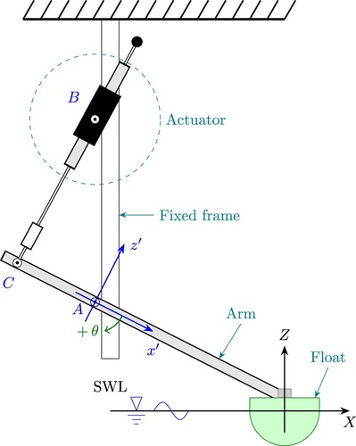
The WEC selected for testing the control algorithm proposed in the present paper is a scaled model of the Wavestar device used in the WEC control competition (Ringwood et al., 2017). The development of the model is kept to a minimum in this Section for brevity. A semi-sphere serves as a floater in this model, and it is attached to a rotating arm, which is hinged at a fixed reference point A (Figure 1). For the float and linkage arm about point A, the device's dynamics can be reduced to an analogous equation-of-motion: (1a) $\begin{array}{rl}(J+J_{\mathrm{\infty }})\ddot{\theta }(t)& =-K_{hs}\theta (t)-b_v\dot{\theta }(t)-M_r(t)-M_{exc}(t)\\ & +M_{pto}(t)\end{array}$(1a) (1b) $\begin{array}{rl}\underset{\_}{\dot{r}}(t)& =A_r\underset{\_}{r}(t)+B_r\dot{\theta }(t)\end{array}$(1b) (1c) $\begin{array}{rl}{M}_r(t)& =C_r\underset{\_}{r}(t)+D_r\dot{\theta }(t)\end{array}$(1c) where:

• θ represents the angular displacement of the arm with respect to the equilibrium position, $\dot{\theta }$ and $\ddot{\theta }$ represent the angular velocity and angular acceleration of the arm.

• J is the total mass moment of inertia of the float and pivot arm.

• $J_{\mathrm{\infty }}$ is the added mass moment of the inertia.

• $K_{hs}$ is the hydrostatic coefficient,

• $b_v$ is a linear damping coefficient (Tom et al., 2018).

• $M_r$ is the radiation moment.

• $M_{exc}$ is the excitation moment due to the incident wave.

• $M_{pto}$ is the PTO moment (input to the system).

• ($A_r,B_r,C_r,D_r$,) are the state space matrices used to approximate the radiation moment $M_r$ avoiding the direct computation of the convolution integral in time-domain simulation. The state vector $\underset{\_}{r}(t)$ have no physical meaning, but still contain information on the condition of the surrounding fluid (Cretel et al., 2010).

Remark 2.1

It is crucial to recall that all of the parameters and variables in Equation (1a(1a) $\begin{array}{rl}(J+J_{\mathrm{\infty }})\ddot{\theta }(t)& =-K_{hs}\theta (t)-b_v\dot{\theta }(t)-M_r(t)-M_{exc}(t)\\ & +M_{pto}(t)\end{array}$(1a) ) are specified w.r.t. the rotating point A. For more details of the model development, the interested reader is referred to Tom, Ruehl, and Ferri (2018) and Tona et al. (2020, august).

Figure 1. Diagram of the Wavestar WEC system.

3. Problem formulation

3.1. General objective

The main objective of a PTO system controller is to transfer as much energy as possible from the waves to the grid for a broad range of sea states. The electrical energy $E_e$ absorbed by the grid over a time horizon T, is defined as: (2) $E_e=-{\int }_t^{t+T}{P}_e(\tau )\mathrm{d}\tau =-{\int }_t^{t+T}\mathrm{\Gamma }(\tau )P_m(\tau )\mathrm{d}\tau$(2) where $P_e$ denotes the electrical power delivered to the grid, $P_m$ the instantaneous hydromechanical power absorbed by the PTO system, Γ the overall efficiency of the PTO system, and τ is the variable of integration.

The negative sign in Equation (2(2) $E_e=-{\int }_t^{t+T}{P}_e(\tau )\mathrm{d}\tau =-{\int }_t^{t+T}\mathrm{\Gamma }(\tau )P_m(\tau )\mathrm{d}\tau$(2) ) is because the energy is drawn from the WEC and thus, the maximisation of the energy absorbed corresponds to a minimisation of the control objective (Nguyen et al., 2016, june).

The instantaneous hydromechanical absorbed power is given by: (3) $P_m(t)=M_{pto}(t)\dot{\theta }(t)$(3) where $M_{pto}$ is the PTO moment and $\dot{\theta }$ represents the angular velocity of the arm. To use standard nomenclature, $M_{pto}(t_k)$ is replaced by $u_k$.

Substituting (3(3) $P_m(t)=M_{pto}(t)\dot{\theta }(t)$(3) ) in (2(2) $E_e=-{\int }_t^{t+T}{P}_e(\tau )\mathrm{d}\tau =-{\int }_t^{t+T}\mathrm{\Gamma }(\tau )P_m(\tau )\mathrm{d}\tau$(2) ) the optimal control problem can be formulated as: (4a) $\begin{array}{rl}\underset{u}{min}& -E_e={\int }_t^{t+T}\mathrm{\Gamma }(\tau )u(\tau )\dot{\theta }(\tau )\mathrm{d}\tau \end{array}$(4a) (4b) $\begin{array}{rl}\mathrm{s}.\mathrm{t}.& \dot{\underset{\_}{x}}(t)=f(\underset{\_}{x},u,w,t)\end{array}$(4b) (4c) $\begin{array}{rl}& U_{min}\le u(t)\le U_{max}\end{array}$(4c)

The equivalent discrete-time optimisation problem is given by: (5a) $\begin{array}{rl}\underset{u_i}{min}& J=\sum _{i=1}^{N_p}{\gamma }_{k+i}{u}_{k+i-1}{\dot{\theta }}_{k+i}\end{array}$(5a) (5b) $\begin{array}{rl}\mathrm{s}.\mathrm{t}.& {\underset{\_}{x}}_{k+1}=f({\underset{\_}{x}}_k,u_k,w_k)\end{array}$(5b) (5c) $\begin{array}{rl}& U_{min}\le u_k\le U_{max}\end{array}$(5c) where $N_p$ is the prediction horizon, Equation (5b(5b) $\begin{array}{rl}\mathrm{s}.\mathrm{t}.& {\underset{\_}{x}}_{k+1}=f({\underset{\_}{x}}_k,u_k,w_k)\end{array}$(5b) ) represents the WEC dynamics, with the states $\underset{\_}{x}=[\theta \dot{\theta }\underset{\_}{r}{]}^{\mathrm{T}}$, $u_k$ the control input, $w_k$ the discrete-time value for the excitation moment $M_{exc}$, and ${\gamma }_k$ the specific value for the PTO efficiency at time instant $t_k$; that is, $\mathrm{\Gamma }(t_k)={\gamma }_k$.

Remark 3.1

Equation (5a(5a) $\begin{array}{rl}\underset{u_i}{min}& J=\sum _{i=1}^{N_p}{\gamma }_{k+i}{u}_{k+i-1}{\dot{\theta }}_{k+i}\end{array}$(5a) ) considers the velocity $\dot{\theta }$ and the control input u at different time steps (k + i and k + i−1). This is chosen to ensure causality of the solution as discussed in Li and Belmont (2014).

3.2. Power take-off efficiency

One of the common control policies proposed to increase the amount of energy extracted from the ocean waves is reactive control. The main idea of this strategy is to match the intrinsic impedance of the system by supplying power to the PTO system for some parts of the sinusoidal cycle (Ringwood et al., 2014). One of the main limitations of reactive control is that it creates a particular demand on PTO systems to allow for bi-directional power flow. Still, it can yield energy losses if it is not tuned correctly (Li & Belmont, 2014; Mérigaud & Tona, 2020; Ringwood et al., 2014).

PTO systems are not perfect in real-world applications, which means that the electrical power $P_e$ is never equal to the absorbed mechanical power $P_m$. In other words, because of the losses that occur throughout the conversion stage, the electrical power available at the end of the mechanical-to-electrical conversion stage is less than the absorbed mechanical power, i.e. $0\le P_e\le P_m$. If a reactive control strategy is adopted, at certain times, the PTO system must return some electric power from the grid back into the ocean ($P_m\le 0$). In those instants, and because of the losses in the conversion stages, the electrical power provided by the grid to the PTO system must be larger than $|P_m|$, i.e. $P_e\le P_m\le 0$ (Mérigaud & Tona, 2020).

Given that the efficiency of the PTO system varies depending on the direction of the energy flow (float-to-grid or grid-to-float directions), the energy-maximising control strategy must consider the efficiency when solving the OCP (Andersen et al., 2015). Other studies have discussed the impact of nonideal PTO efficiency on WEC control (Bacelli et al., 2015; Falcão & Henriques, 2015, august; Genest et al., 2014; Mérigaud & Tona, 2020; Sanchez et al., 2015; Tedeschi et al., 2011; Tom et al., 2019; Tona et al., 2015, 2019), with the main drawback that none of them solves the OCP related to the nonlinear output equation of the model in real-time (see Section 4.1, Equation (8(8) $y_k=g_k=\left[\begin{array}{c}{\dot{\theta }}_k\\ {\gamma }_k{u}_{k-1}\end{array}\right]$(8) )), which is the main contribution of this paper.

The PTO system efficiency can be modelled by a modification of a step function, having two different values for the efficiency depending if the PTO system is working as motoring (grid-to-float) or as generator (float-to-grid). Using this modified-step function model, the instantaneous power extracted is given by: (6) $P_e(t)=\mathrm{\Gamma }(t)P_m(t),\{\begin{array}{ll}\mathrm{\Gamma }(t)={\mu }_{gen}& \mathrm{if}{P}_m(t)\ge 0\\ \mathrm{\Gamma }(t)={\mu }_{mot}& \mathrm{if}{P}_m(t)<0\end{array}$(6) where ${\mu }_{gen}$ is the global efficiency of the PTO system when it delivers energy to the grid and ${\mu }_{mot}$ is the global efficiency when the PTO system consumes energy from the grid.

4. Nonlinear model predictive control

Because of its ability to explicitly handle constraints and nonlinear dynamics that define the system of interest, NMPC is becoming increasingly popular for real-time optimal control solutions (Diehl et al., 2005). The following subsections are intended to offer a quick overview of each of the steps/phases involved in developing NMPC.

Let us first define some notations used in the following subsections. The upper bar $(\overline{x})$ represents a nominal-guessed point which is considered a ‘desirable-optimal’ trajectory to be used by the NMPC framework to optimise and improve the solution iteratively. Similarly, the hat $(\hat{x})$ represents the predicted, whilst the variable without any additional notation will be reserved for the real/simulated value. Also, the underbar notation for vectors $(\underset{\_}{x})$ will be dropped for the sake of readability and to simplify the notation of the following equations.

4.1. Modelling

In this paper, we consider a general ordinary differential equation describing the system evolution in continuous time of a generic wave energy converter on a time interval $[0,T]$ of the form: (7a) $\begin{array}{rl}\dot{x}(t)& =f(x(t),u(t),w(t),t),t\in [0,T]\end{array}$(7a) (7b) $\begin{array}{rl}y(t)& =g(x(t),u(t),w(t),t)\end{array}$(7b) where $t\in \mathbb{R}$ is the time, $u(t)\in {\mathbb{R}}^{n_u}$ are the control input, $x(t)\in {\mathbb{R}}^{n_x}$ is the state, $w(t)\in {\mathbb{R}}^{n_w}$ is wave excitation input, and $y(t)\in {\mathbb{R}}^{n_y}$. The function f is a map from states, control input, wave input, and time to the rate of change of the state, i.e. $f:{\mathbb{R}}^{n_x}\times {\mathbb{R}}^{n_u}\times {\mathbb{R}}^{n_w}\times [0,T]\mapsto {\mathbb{R}}^{n_x}$. Similar definition for g. Also it is assume that f and g are continuous with respect to x and t.

The prediction and optimisation presented in Sections 4.2 and 4.3 respectively, are formulated in discrete time, therefore to translate the continuous-time model into the discrete-time model, a discretisation by integration is implemented (González-Villarreal, 2021). For this study, we decided to use the explicit 4th order Runge-Kutta method.

In the present study, the output function $g(x_k,u_k,w_k)$ is selected as follows: (8) $y_k=g_k=\left[\begin{array}{c}{\dot{\theta }}_k\\ {\gamma }_k{u}_{k-1}\end{array}\right]$(8) On the other hand, the PTO efficiency model presented in Equation (6(6) $P_e(t)=\mathrm{\Gamma }(t)P_m(t),\{\begin{array}{ll}\mathrm{\Gamma }(t)={\mu }_{gen}& \mathrm{if}{P}_m(t)\ge 0\\ \mathrm{\Gamma }(t)={\mu }_{mot}& \mathrm{if}{P}_m(t)<0\end{array}$(6) ) suffers from a discontinuity between the two cases $P_m(t)\ge 0$ and $P_m(t)<0$. In gradient-based optimisation approaches, such a discontinuous function is undesirable. Therefore, a smoothed approximation to Equation (6(6) $P_e(t)=\mathrm{\Gamma }(t)P_m(t),\{\begin{array}{ll}\mathrm{\Gamma }(t)={\mu }_{gen}& \mathrm{if}{P}_m(t)\ge 0\\ \mathrm{\Gamma }(t)={\mu }_{mot}& \mathrm{if}{P}_m(t)<0\end{array}$(6) ), continuous in $P_m(t)=0$, must be implemented to prevent problems with the optimisation technique.

A modified-hyperbolic tangent function is used to approximate Equation (6(6) $P_e(t)=\mathrm{\Gamma }(t)P_m(t),\{\begin{array}{ll}\mathrm{\Gamma }(t)={\mu }_{gen}& \mathrm{if}{P}_m(t)\ge 0\\ \mathrm{\Gamma }(t)={\mu }_{mot}& \mathrm{if}{P}_m(t)<0\end{array}$(6) ) in Mérigaud and Tona (2020) and Tona et al. (2015). Although a sigmoid function or another comparable activation function may be used to approximate this sort of discontinuous function, the approximation using tanh is preserved in this study and is given by: (9) ${\mathrm{\Gamma }}_{approx}(t)=\alpha +\beta \tanh (\phi P_m(t))$(9) where α is an offset, β is a scaling factor, and φ is a real positive parameter that determines the accuracy of the approximation. Defined as $\alpha =({\mu }_{mot}+{\mu }_{gent})/2$, and $\beta =({\mu }_{mot}-{\mu }_{gent})/2$.

4.2. Prediction

The derivation of the prediction model discussed in this Section follows a similar pattern to that presented in González-Villarreal and Rossiter (2020b) and is presented here to allow the contents of this paper to be self-contained. Using a first order multivariable Taylor series expansion, the linearised model for Equation (7a(7a) $\begin{array}{rl}\dot{x}(t)& =f(x(t),u(t),w(t),t),t\in [0,T]\end{array}$(7a) ) at time step k, is given by: (10) ${\hat{x}}_{k+1}={\overline{x}}_{k+1}+A_k\delta {\hat{x}}_k+B_k\delta {\hat{u}}_k+B_{w,k}\delta {\hat{w}}_k$(10) where $\delta {\hat{x}}_k={\hat{x}}_k-{\overline{x}}_k$, $\delta {\hat{u}}_k={\hat{u}}_k-{\overline{u}}_k$, and $\delta {\hat{w}}_k={\hat{w}}_k-{\overline{w}}_k$ are the deviations of the state, control input and wave excitation moment from their nominal points $(\overline{x_k},\overline{u_k},\overline{w_k})$ at time step t = k respectively, and $A_k$, $B_k$, and $B_{w,k}$ are the partial derivatives w.r.t. the states, control input, and wave excitation input moment, which will be defined shortly.

The wave excitation moment deviation $\delta {\hat{w}}_k$ requires special consideration at this stage. The approach used in this work assumes that the wave excitation moment at the current time and for a specific time horizon is known at each time step. Therefore, the nominal and predicted trajectory for the wave excitation moment is the same at each time step, i.e. $\delta {\hat{w}}_k=0$ for all k, and thus the following derivation does not take this term into account. But practical implementation could take deviations into account, which could emerge considering a correction-estimation of the predicted wave during the feedback phase. $\begin{array}{cc}{A}_k={\frac{\mathrm{\partial }f(x,u,w)}{\mathrm{\partial }x}|}_{\begin{array}{c}{\overline{x}}_k\\ {\overline{u}}_k\\ {\overline{w}}_k\end{array}}& B_k={\frac{\mathrm{\partial }f(x,u,w)}{\mathrm{\partial }u}|}_{\begin{array}{c}{\overline{x}}_k\\ {\overline{u}}_k\\ {\overline{w}}_k\end{array}}\\ {\overline{x}}_{k+1}=f({\overline{x}}_k,{\overline{u}}_k,{\overline{w}}_k)& \end{array}$The deviation $\delta x_{k+1}=x_{k+1}-{\overline{x}}_{k+1}$ at time step t = k + 1 can be approximated by: (11) $\delta {\hat{x}}_{k+1}=A_k\delta {\hat{x}}_k+B_k\delta {\hat{u}}_k$(11) Given that the nominal point ${\overline{x}}_{k+1}$ and the linearisation matrices $A_k,B_k$ are parametrically dependent on ${\overline{x}}_k,{\overline{u}}_k,{\overline{w}}_k$, and that the value for $x_k$ and ${\overline{w}}_k$ are already known at a given sampling time t = k (either by measurements or by state estimation), the value for ${\overline{x}}_{k+1}$ can only be computed if the value for the optimal control input ${\overline{u}}_k$ is known. Similar for ${\overline{x}}_{k+2}$, for which the value of ${\overline{u}}_{k+1}$ is needed.

If values for the future optimal-nominal input trajectory $\overline{U}=[{\overline{u}}_k^T,{\overline{u}}_{k+1}^T,\dots ,{\overline{u}}_{k+N_p-1}^T{]}^T$ are assumed or guessed, the projected nominal state trajectory $\overline{X}=[{\overline{x}}_{k+1}^T,{\overline{x}}_{k+2}^T,\dots ,{\overline{x}}_{k+N_p}^T{]}^T$ and the linearisation matrices $A_k,B_k$ can be computed for future time steps $t=k+1,k+2,\dots ,k+N_p$, where $N_p$ is known as the prediction horizon. A typical strategy to guess the nominal input trajectory $\overline{U}$ (no necessarily the optimum) is to simulate the system in free response, i.e. $\overline{U}=[0_0,\dots ,0_{Np-1}]$ for k = 0, the system is linearised around the resulting state trajectory, and the optimisation improves the initial guess at every iteration using a Newton-type framework (Diehl et al., 2005; Gros et al., 2016). This technique is often referred as single-shooting. Other techniques such as multiple shooting and collocation points can also be used with the proposed approach (Quirynen et al., 2015).

After obtaining $\overline{X}$ with $\overline{U}$, Equation (11(11) $\delta {\hat{x}}_{k+1}=A_k\delta {\hat{x}}_k+B_k\delta {\hat{u}}_k$(11) ) can be shifted forward: (12) $\delta {\hat{x}}_{k+2}=A_{k+1}\delta {\hat{x}}_{k+1}+B_{k+1}\delta {\hat{u}}_{k+1}$(12) Substituting Equation (11(11) $\delta {\hat{x}}_{k+1}=A_k\delta {\hat{x}}_k+B_k\delta {\hat{u}}_k$(11) ) into Equation (12(12) $\delta {\hat{x}}_{k+2}=A_{k+1}\delta {\hat{x}}_{k+1}+B_{k+1}\delta {\hat{u}}_{k+1}$(12) ) yields: (13) $\delta {\hat{x}}_{k+2}=A_{k+1}(A_k\delta {\hat{x}}_k+B_k\delta {\hat{u}}_k)+B_{k+1}\delta {\hat{u}}_{k+1}$(13) By recursively repeating the preceding procedure for $N_p$ steps and considering just the system output (Equation (8(8) $y_k=g_k=\left[\begin{array}{c}{\dot{\theta }}_k\\ {\gamma }_k{u}_{k-1}\end{array}\right]$(8) )), the predicted deviations from the nominal output trajectory may be expressed in a matrix form by: (14) $\delta \hat{Y}=G_y\delta x_k+H_y\delta \hat{U}$(14) where $\delta \hat{Y}=\hat{Y}-\overline{Y}=[\delta y_{k+1}^T,\delta y_{k+2}^T,\dots ,\delta y_{k+N_p}^T{]}^{\mathrm{T}}$ are the output deviations, $\delta \hat{U}=\hat{U}-\overline{U}=[\delta {\hat{u}}_k^T,\delta {\hat{u}}_{k+1}^T,\dots ,\delta {\hat{u}}_{k+N_p-1}^T{]}^{\mathrm{T}}$ are the control input deviations. The matrices $G_y$ and $H_y$ are given by: (15) $G_y=\left[\begin{array}{c}{C}_1{A}_0\\ C_2{A}_1{A}_0\\ ⋮\\ C_{N_p}{A}_{N_p-1}\cdots A_1{A}_0\end{array}\right]$(15) (16) $H_y=\left[\begin{array}{cccc}{C}_1{B}_0& \mathbf{0}& \cdots & \mathbf{0}\\ C_2{A}_1{B}_0& C_2{B}_1& \cdots & ⋮\\ C_3{A}_2{A}_1{B}_0& C_3{A}_2{B}_1& \ddots & \mathbf{0}\\ ⋮& ⋮& \ddots & ⋮\\ C_{N_p}{A}_{N_p-1}\cdots A_1{B}_0& C_{N_p}{A}_{N_p-1}\cdots A_2{B}_1& \cdots & C_{N_p}{B}_{N_p-1}\end{array}\right]$(16) The dimensions for these matrices are $G_y=[N_p{n}_y\times n_x]$, $H_y=[N_p{n}_y\times N_p{n}_u]$, and $C_k$ is the partial derivative of Equation (8(8) $y_k=g_k=\left[\begin{array}{c}{\dot{\theta }}_k\\ {\gamma }_k{u}_{k-1}\end{array}\right]$(8) ) w.r.t. nominal state, evaluated at the specific time step t = k, and is given by: $C_k={\frac{\mathrm{\partial }g(x,u,w)}{\mathrm{\partial }x}|}_{\begin{array}{c}{\overline{x}}_k\\ {\overline{u}}_k\\ {\overline{w}}_k\end{array}}$In addition, the matrix $\mathbf{0}$ represents a matrix of zeros with the same dimensions as the matrix $C_k{B}_k$.

4.3. Optimisation

Following the definition of the prediction models, the cost function described in Equation (5a(5a) $\begin{array}{rl}\underset{u_i}{min}& J=\sum _{i=1}^{N_p}{\gamma }_{k+i}{u}_{k+i-1}{\dot{\theta }}_{k+i}\end{array}$(5a) ) can be recast as follows: (17) $J=\frac{1}{2}{\hat{Y}}^{T}Q\hat{Y}+\frac{1}{2}\delta {\hat{U}}^{T}R\delta \hat{U}$(17) where the matrix R is a positive definite matrix with dimensions $[N_p{n}_u\times N_p{n}_u]$ and constant elements over its diagonal. Q is selected as a block diagonal matrix with dimensions $[N_p{n}_u\times N_p{n}_u]$ and inner matrices $q_i$ used to compute the product ${\dot{\theta }}_k\times {\gamma }_k{u}_{k-1}$ as defined in Guerrero-Fernández et al. (2020). (18) $Q=\left[\begin{array}{cccc}{q}_1& \mathbf{0}& \cdots & \mathbf{0}\\ \mathbf{0}& q_2& \ddots & ⋮\\ ⋮& \ddots & \ddots & \mathbf{0}\\ \mathbf{0}& \cdots & \mathbf{0}& q_{N_p}\end{array}\right]\begin{array}{c}{q}_i=\left[\begin{array}{cc}0& 1\\ 1& 0\end{array}\right]\\ \mathrm{\forall }i=[1,N_p]\end{array}$(18) The reader may have observed that, in addition to the condensed format of (17(17) $J=\frac{1}{2}{\hat{Y}}^{T}Q\hat{Y}+\frac{1}{2}\delta {\hat{U}}^{T}R\delta \hat{U}$(17) ), the cost differs from (5a(5a) $\begin{array}{rl}\underset{u_i}{min}& J=\sum _{i=1}^{N_p}{\gamma }_{k+i}{u}_{k+i-1}{\dot{\theta }}_{k+i}\end{array}$(5a) ) in that it includes an additional term that penalises the input deviation. The input deviation term is included for two reasons: first, it smooths the control signal, making the requirement for the actuator's response limit less stringent, and second, according to Ringwood et al. (2014), Li and Belmont (2014), Mérigaud and Tona (2020) and Bacelli and Coe (2021), a reactive control strategy with a cost function based solely on maximising the extracted energy can result in overall negative energy absorbed, implying that the system is losing energy rather than absorbing energy from the waves.

Finally, the standard quadratic programming (QP) formulation is obtained by substituting the linearised output prediction Equation (14(14) $\delta \hat{Y}=G_y\delta x_k+H_y\delta \hat{U}$(14) ) in Equation (17(17) $J=\frac{1}{2}{\hat{Y}}^{T}Q\hat{Y}+\frac{1}{2}\delta {\hat{U}}^{T}R\delta \hat{U}$(17) ), grouping similar terms w.r.t. the decision variable $\delta \hat{U}$, and omitting any constant terms in the cost function: (19a) $\begin{array}{rl}J& =\frac{1}{2}\delta {\hat{U}}^{T}E\delta \hat{U}+\delta {\hat{U}}^{T}f\mathrm{s}.\mathrm{t}.M\delta \hat{U}\le \rho \end{array}$(19a) (19b) $\begin{array}{rl}E& =H_y^{T}Q{H}_y+R\end{array}$(19b) (19c) $\begin{array}{rl}f& =H_y^{T}Q[\overline{Y}+G_y\delta x_k]\end{array}$(19c) where $E\in {\mathbb{R}}^{N_p{n}_u\times N_p{n}_u}$ is a symmetric matrix known as the hessian and $f\in {\mathbb{R}}^{N_p{n}_u}$ is a column vector usually referred as the linear term; $M\in {\mathbb{R}}^{2N_p{n}_u\times N_p{n}_u}$ is the constraints matrix and $\rho \in {\mathbb{R}}^{2N_p{n}_u}$ is the constraints vector, defined as: (20) $M=\left[\begin{array}{c}I\\ -I\end{array}\right]\rho =\left[\begin{array}{c}{U}_{max}-\overline{U}\\ -(U_{min}-\overline{U})\end{array}\right]$(20) Here, the matrix M and the vector ρ are defined considering only constraints in the control input. If constraints for any states are required, M and ρ must be slightly reformulated. The reader may have also noticed that $G_y$ and $H_y$, therefore E and f, are time-dependent, which is one of the main reasons why NMPC is computationally expensive.

After defining E, f, M, and ρ, the OCP can be solved using any QP solver, such as Matlab's quadprog function, qpOASES (Ferreau et al., 2008), and so on. In this study, qpOASES was used. Once the QP problem has been solved, the new control input sequence is computed, recalling that $\hat{U}=\overline{U}+\delta U$. Only the first input is applied to the system, and the procedure is repeated at the next time step, which is known as the receding horizon scheme (González-Villarreal & Rossiter, 2020a).

4.4. Real-time iterations scheme

In this Section, we recall the RTI scheme first introduced by Diehl et al. (2005). A fully converged NMPC should ideally re-linearise the predictions and thus cost function Equation (19a(19a) $\begin{array}{rl}J& =\frac{1}{2}\delta {\hat{U}}^{T}E\delta \hat{U}+\delta {\hat{U}}^{T}f\mathrm{s}.\mathrm{t}.M\delta \hat{U}\le \rho \end{array}$(19a) ) until no deviations are necessary, i.e. $\delta \hat{U}=\mathbf{0}$ (González-Villarreal & Rossiter, 2020a). is not computationally tractable in real-time applications since one must provide a solution at each time step under strict time constraints and avoid solving a problem that is just ‘getting older’ (Gros et al., 2016).

The RTI exploits the fact that NMPC is required to solve optimisations closely related from one-time step to the next, which has proven to be a very successful and popular method of tackling the problem at hand. The RTI scheme is summarised in the following subsections.

4.4.1. Initial value embedding

Choosing an appropriate initial estimate for $\hat{U}$ optimal, denoted as ${\hat{U}}^{\ast }$, is critical for fast and reliable convergence of the sequential quadratic programming (SQP) approach. It can help avoid a premature exit from the SQP algorithm with an infeasible solution, but also it allows for complete Newton steps in the SQP, which yields a fast convergence rate (Gros et al., 2016). To facilitate the estimation, the previous optimal input trajectory is utilised in a shifted version to hot-start the solution at the following sampling time, generally by duplicating the last value. In the case of active-set-based SQP, the Lagrange multipliers λ, linked to the optimisation constraints, may also be used to hot-start the QP in a shifted version (González-Villarreal & Rossiter, 2020b).

4.4.2. Single sequential quadratic programming iteration

One of the most efficient approaches to handle nonlinear programming (NLP) problems is sequential quadratic programming (SQP) (Nocedal, 2006). In the SQP approach, the NLP is sequentially approximated by QPs, delivering Newton directions for performing steps towards the solution starting from the available guess. Iterations are performed until convergence is reached, taking (not necessarily full) Newton steps (Gros et al., 2016). However, within the RTI scheme, only one iteration of SQP is performed, given that the optimisation is ‘warn-started’ from the prior solution (González-Villarreal & Rossiter, 2020b).

4.4.3. Computation separation

The separation of the computation is perhaps the essential aspect of the RTI scheme. It divides the calculations into preparation and feedback phases. A timing diagram that illustrates this can be seen in Gros et al. (2016).

• Preparation phase: It uses the last applied input trajectory $u_{k-1}$ to predict the state ${\hat{\overline{x}}}_{k|k-1}$, which is then used to linearise and prepare a QP to be later solved in the feedback phase.

• Feedback phase: as soon as the state $x_k$ becomes available, the state deviation $\delta x_k=x_k-{\hat{\overline{x}}}_{k|k-1}$ is used to complete the calculation of f, ρ and the optimal correction $\delta {\hat{U}}^{\ast }$ to the current trajectory $\hat{U}$.

4.5. Efficient algorithm $O(N^2)$ to compute the hessian E

Because of its dimensions and time-varying nature, the hessian E is one of the most computationally expensive operations of the OCP mentioned above. Fortunately, the underlying structure of the matrix $H_y$ allows the implementation of the so-called $O(N^2)$ condensing algorithm, initially presented in Andersson (2013) and re-derived in González-Villarreal (2021). It provides an efficient calculation of the hessian term $H_y^{T}Q{H}_y$ via a recursive-like operation that takes advantage of the block triangular structure of matrix $H_y$ to avoid the zero terms computations, as well as any repeated terms that may result from the direct calculation. However, the condensing algorithm $O(N^2)$ presented in the preceding studies was derived for quadratic optimisations considering states/inputs and state-input costs, whereas, for the formulation presented in this paper, an algorithm for ‘output-only’ cost functions is required.

For the sake of simplicity, the algorithm is derived here considering the resulting hessian with a short horizon of $N_p=3$. $\begin{array}{rl}E& =\underset{H_y}{\underbrace{{\left[\begin{array}{ccc}{C}_1{B}_0& 0& 0\\ C_2{A}_1{B}_0& C_2{B}_1& 0\\ C_3{A}_2{A}_1{B}_0& C_3{A}_2{B}_1& C_3{B}_2\end{array}\right]}^{\mathrm{T}}}}\underset{Q}{\underbrace{\left[\begin{array}{ccc}{q}_1& 0& 0\\ 0& q_2& 0\\ 0& 0& q_3\end{array}\right]}}\\ & \underset{H_y}{\underbrace{\left[\begin{array}{ccc}{C}_1{B}_0& 0& 0\\ C_2{A}_1{B}_0& C_2{B}_1& 0\\ C_3{A}_2{A}_1{B}_0& C_3{A}_2{B}_1& C_3{B}_2\end{array}\right]}}\\ E& =\left[\begin{array}{ccc}{E}_{1,1}& E_{1,2}& E_{1,3}\\ E_{2,1}& E_{2,2}& E_{2,3}\\ E_{3,1}& E_{3,2}& E_{3,3}\end{array}\right]\end{array}$One can see that a good starting point towards computing the hessian is the multiplication of $Q{H}_y$. The resulting matrix S is given by: (21) $S=\left[\begin{array}{ccc}{s}_{1,1}& 0& 0\\ s_{2,1}& s_{2,2}& 0\\ s_{3,1}& s_{3,2}& s_{2,3}\end{array}\right]=\left[\begin{array}{ccc}{q}_1{C}_1{B}_0& 0& 0\\ q_2{C}_2{A}_1{B}_0& q_2{C}_2{B}_1& 0\\ q_3{C}_3{A}_2{A}_1{B}_0& q_3{C}_3{A}_2{B}_1& q_3{C}_3{B}_2\end{array}\right]$(21) Separating the hessian column-wise, the first column of it is computed as follows: (22) $\left[\begin{array}{c}{E}_{1,1}\\ E_{2,1}\\ E_{3,1}\end{array}\right]=\left[\begin{array}{ccc}{B}_0^T{C}_1^T& B_0^T{A}_1^T{C}_2^T& B_0^T{A}_1^T{A}_2^T{C}_3^T\\ 0& B_1^T{C}_2^T& B_1^T{A}_2^T{C}_3^T\\ 0& 0& B_2^T{C}_3^T\end{array}\right]\left[\begin{array}{c}{s}_{1,1}\\ s_{2,1}\\ s_{3,1}\end{array}\right]$(22) The algorithm is based on iteratively reusing terms that were computed previously. Starting from the last term $E_{3,1}$: $\begin{array}{rl}{E}_{3,1}& =B_2^T{C}_3^T{s}_{3,1}\mapsto Z_{3,1}=C_3^T{s}_{3,1}\\ E_{3,1}& =B_2^T{Z}_{3,1}\end{array}$The next term $E_{2,1}$ is computed as: $E_{2,1}=B_1^T{C}_2^T{s}_{2,1}+B_1^T{A}_2^T{C}_3^T{s}_{3,1}$Reusing the term $Z_{3,1}$ computed previously: $\begin{array}{rl}{E}_{2,1}& =B_1^T(C_2^T{s}_{2,1}+A_2^T{Z}_{3,1})\mapsto Z_{2,1}=C_2^T{s}_{2,1}+A_2^T{Z}_{3,1}\\ E_{2,1}& =B_1^T{Z}_{2,1}\end{array}$Using the same logic, the last term $E_{1,1}$ can be calculated as function of $Z_{2,1}$, and hence of $Z_{3,1}$: $\begin{array}{rl}{E}_{1,1}& =B_0^T(C_1^T{s}_{1,1}+A_1^T{Z}_{2,1})\mapsto Z_{1,1}=C_1^T{s}_{1,1}+A_1^T{Z}_{2,1}\\ E_{1,1}& =B_0^T{Z}_{1,1}\end{array}$Thus, an obvious pattern can be seen where the hessian can be calculated by recursively computing the terms with an expression like $Z_{k,j}=C_k^T{s}_{k,j}+A_j^T{Z}_{k+1,j}$ for $k,j\in [1,\dots ,N_p\times n_u]$, and then calculating the hessian term $E_{k,j}=B_{k-1}^T{Z}_{k,j}$. Keeping in mind that in the case where k = j, the term $R(k,j)$ needs to be added to $E_{k,j}$, i.e. to the diagonal of the hessian, see Equation (19b(19b) $\begin{array}{rl}E& =H_y^{T}Q{H}_y+R\end{array}$(19b) ).

Because the hessian is symmetric (Nocedal, 2006), the final algorithm only calculates the lower triangular terms and duplicates the rest of the terms.

Finally, this approach can also be used to re-derive the algorithm $O(N)$ (Andersson, 2013), which can be used to calculate the linear term f, see Equation (19c(19c) $\begin{array}{rl}f& =H_y^{T}Q[\overline{Y}+G_y\delta x_k]\end{array}$(19c) ), for ‘output-only’ cost functions.

5. Numerical results

In this section, numerical results of the proposed control strategy implemented on the benchmark scale model of the Wavestar (Ringwood et al., 2017) are presented.

5.1. Model parameters

The model parameters used in this study are summarised in Table 1.

Table 1. Model parameters for the scale model of the Wavestar device, taken from Tona et al. (2019) and Ringwood et al. (2017).

Hydrodynamic parameters
Inertia of arm and float	J	$1.04\mathrm{kg}{\mathrm{m}}^2$
Added inertia	$J_{\mathrm{\infty }}$	$0.4805\mathrm{kg}{\mathrm{m}}^2$
Hydrostatic stiffness coefficient	$K_{hs}$	$92.33\mathrm{N}\mathrm{m}{\mathrm{rad}}^{-1}$
Rotational linear damping	$b_v$	$1.80\mathrm{N}\mathrm{m}{\mathrm{rad}}^{-1}{\mathrm{s}}^{-1}$
Radiation moment impulse response realisation
$A_r=\left[\begin{array}{cc}-13.59& -13.35\\ 8.00& 0.00\end{array}\right]$	$B_r\left[\begin{array}{c}8.0\\ 0.0\end{array}\right]$
$C_r=\left[\begin{array}{cc}4.739& 0.5\end{array}\right]$	$D_r=-0.1586$

5.2. Wave conditions

The wave climate is characterised by the significant wave height $H_{m0}$, the peak wave period $T_p$ and the wave direction. A series of three unidirectional sea states, generated using the JONSWAP spectrum, are used for this study. The spectrum parameters are given in Table 2, based on the sea states used in the WECCCOMP (Tona et al., 2019).

Table 2. Parameters for wave generation using JONSWAP spectrum. Significant wave height $H_{m0}$, peak period $T_p$ and peak enhancement factor γ.

Name${}^{\mathrm{a}}$	$H_{m0}$ [m]	$T_p$ [s]	γ [-]	Duration [s]
SS4	0.0208	0.988	3.3	98.8
SS5	0.0625	1.412	3.3	141.2
SS6	0.1042	1.836	3.3	183.6

${}^{\mathrm{a}}$Names are given to have consistency with the names given in the WECCCOMP (Tona et al., 2019).

5.3. Simulation and control parameters

Given that the main goal of this work is to evaluate the RTI-NMPC proposed for WECs, all simulation trials were done in the nominal case, i.e. no noise or uncertainty was included. It was also assumed that the vector containing the future wave excitation moment is known throughout the prediction horizon.

Regarding the prediction horizon, research on wave excitation force prediction suggests that prediction strategies can predict wave excitation force for swell waves extremely accurately up to two peak wave periods in the future (Fusco & Ringwood, 2010). In light of the foregoing, a prediction horizon equivalent to two peak wave periods ($N_p=2\times T_p/dt$.) was chosen for each sea state. Other relevant control tuning parameters are summarised in Table 3.

Table 3. Simulation and control tuning parameters

Parameter	Value
Simulation time [s]	$100\times T_p$
Control sampling time [ms]	10
Prediction horizon [samples]${}^{⊛}$	Round$(2\times Tp/dt,5)$
${\mu }_{gen}^{\star }$	0.7
${\mu }_{mot}^{\star }$	${0.7}^{-1}$
φ†	1000
Control limit [N m]	±12

$\star$Suggested by Ringwood et al. (2017).

$†$Used in PTO efficiency function approximation.

$⊛$Operator $Round(number,multiple)$ returns a number rounded to the desired multiple.

5.4. Results on the amount of energy absorbed

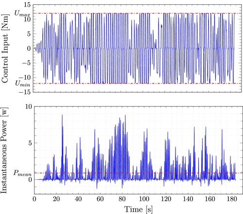
With the idea to have a reference point for each sea state, simulations were carried out using NMPC with an efficiency of $100\mathrm{\%}$. This will give us an estimate of how much energy can be harvested in the case of an ideal bi-directional PTO system.

Figure 2 shows the absorbed power over the simulation time for the sea state SS6. For this simulation, the absorbed energy was 249.75 J with a mean power of 1.4988 W.

Figure 2. Control input and absorbed power by the Wavestar model undersea state SS6 with an ideal bidirectional PTO system. The red dashed line represents the mean absorbed power.

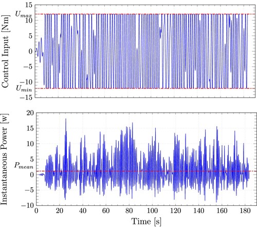
Figure 2 also shows how the control input takes the form of a bang-bang type of control, mostly assigning the values of $u_k=\pm 12$. Similar results were obtained for sea states SS4 and SS5, summarised in Table 4.

Table 4. Energy absorbed and mean power for the sea states considering an ideal bidirectional PTO System.

Sea State	Energy Absorbed [J]	Mean Power [W]
SS4	2.90	0.0366
SS5	71.78	0.5820
SS6	249.75	1.4988

After establishing a reference point for each sea state, further simulations were run with the specified value for PTO system efficiency (see Table 3).

Figure 3 depicts the absorbed power by the WEC model across the simulation time with a cost function without the matrix R (See Equation (19a(19a) $\begin{array}{rl}J& =\frac{1}{2}\delta {\hat{U}}^{T}E\delta \hat{U}+\delta {\hat{U}}^{T}f\mathrm{s}.\mathrm{t}.M\delta \hat{U}\le \rho \end{array}$(19a) )), which penalises the input deviation. Figure 3 and Table 5 complement prior studies (Bacelli & Coe, 2021; Li & Belmont, 2014; Mérigaud & Tona, 2020; Ringwood et al., 2014) where energy loss was reported. Even when considering the PTO system efficiency in the OCP at each sample time, a reactive control strategy can result in overall negative energy absorbed if not correctly tuned.

Figure 3. Control input and absorbed energy by the PTO system with an efficiency value as presented in Table 3 and a cost function without the matrix R for sea state SS6. The mean delivered power is $-0.0087$ W and absorbed energy of $-7.8038$ J, which represent a loss of energy.

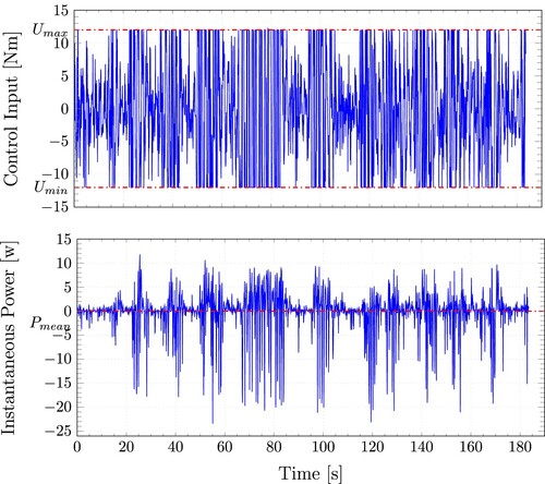
Table 5. Energy absorbed and mean power for the sea states for a nonideal bidirectional PTO System using a cost function inside RTI-NMPC control strategy without the matrix R.

Sea State	Energy Absorbed [J]	Mean Power [W]
SS4	−65.3	−0.6234
SS5	−46.4	−0.3252
SS6	−7.8038	−0.0087

Another insight we can get from Figure 3 is that, even when the control input constraints are met, the input trajectory does not appear acceptable due to the fast change in its value, resulting in severe mechanical wear of the actuator, shortening its life cycle. Hence, there needs to be a trade-off between energy capture and actuator activity in practice.

On the other hand, Figure 4 depicts the control input and the absorbed power for sea state SS6 across the simulation time after simulating the system with a cost function as described in Equation (19a(19a) $\begin{array}{rl}J& =\frac{1}{2}\delta {\hat{U}}^{T}E\delta \hat{U}+\delta {\hat{U}}^{T}f\mathrm{s}.\mathrm{t}.M\delta \hat{U}\le \rho \end{array}$(19a) ).

Figure 4. Control input and absorbed power by the Wavestar model undersea state SS6 using a cost function without considering the matrix R that penalises the input slew rate.

From the data depicted in Figure 4 we can make the following remarks. First, it is clear that the proposed control strategy is successful in absorbing a net positive power from the ocean waves; second, in contrast to the findings in Figure 3, RTI-NMPC with the added weighting matrix R strives to avoid consuming energy from the grid; and third, one can see how the control input is smoother for RTI-NMPC with the added weighting matrix R compared with the one presented in Figure 3 (the reader may consider the resolution for the time length shown in both figures). For sea states SS4 and SS5, similar findings are obtained with cost function (19a(19a) $\begin{array}{rl}J& =\frac{1}{2}\delta {\hat{U}}^{T}E\delta \hat{U}+\delta {\hat{U}}^{T}f\mathrm{s}.\mathrm{t}.M\delta \hat{U}\le \rho \end{array}$(19a) ), these are presented in Table 6.

Table 6. Energy absorbed and mean power for resistive control, MPC, and RTI-NMPC for each sea state.

	Resistive		MPC		RTI – NMPC
Sea State	Absorbed Energy [J]	Mean Power [W]	Absorbed Energy [J]	Mean Power [W]	Absorbed Energy [J]	Mean Power [W]
SS4	1.4974	0.01899	1.1914	0.01537	1.9499	0.02458
SS5	18.2770	0.1468	−13.1914	−0.1083	40.875	0.3210
SS6	59.0760	0.3566	51.0505	0.3532	147.092	0.8897

Now, to compare the control strategy proposed around RTI-NMPC with the added weighting matrix R, two additional sets of simulations were performed using a linear model predictive controller (MPC) and a proportional controller, also known as resistive control in the ocean wave energy community (Maria-Arenas et al., 2019; Sanchez et al., 2015; Wang et al., 2018).

The advantage of employing a resistive control is that it is computationally cheap, i.e. speedy and physically simple to implement, for example, with electronic components. Still, the disadvantage is that it is suboptimal, and the proportional gain must be adjusted for each specific sea state. MPC, on the other hand, even though it attempts to provide an optimal solution at each sample time, the absence of the PTO system efficiency in the OCP renders its solution meaningless at the current time step, resulting in a suboptimal control law, or even in a net negative absorbed energy, depending on the sea state and tuning parameters used in the simulation. For comparative purposes, Figure 5 shows the control input and absorbed power by the Wavestar model for sea state SS6. Figure 6 shows the energy absorbed by the WEC for each control strategy.

Figure 5. Control input and absorbed power by the Wavestar model undersea state SS6 with different control strategies. In blue NMPC using the modified cost function Equation (17(17) $J=\frac{1}{2}{\hat{Y}}^{T}Q\hat{Y}+\frac{1}{2}\delta {\hat{U}}^{T}R\delta \hat{U}$(17) ), in black MPC and red resistive control proportional.

Figure 6. Energy absorbed by the Wavestar model undersea state SS6 with different control strategies. In blue RTI-NMPC using the modified cost function Equation (17(17) $J=\frac{1}{2}{\hat{Y}}^{T}Q\hat{Y}+\frac{1}{2}\delta {\hat{U}}^{T}R\delta \hat{U}$(17) ), in black MPC and red resistive control. The value in parenthesis represents the percentage of energy absorbed concerning the maximum theoretical amount, 249.5 J.

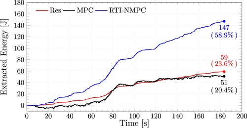
The reader may also see in Figure 6 the percentage of energy absorbed in comparison to the ideal scenario with an efficiency of 100%. From there, we can observe that, while the proportion of energy collected by RTI-NMPC is low in general, 58.9% of 249.5 J, it is significantly higher when compared to the other two control laws considered, 20.4% for MPC and 23.6% for the resistive controller. Between them, RTI-NMPC can absorb roughly three times more than the MPC and two and a half times more than the resistive controller.

Another interesting fact we can extract from these results is that standard MPC, which is well understood and highly praised for linear systems, could not extract more energy than a simple resistive controller. So, linear MPC is not worth the effort, especially considering the extra costs when designing/buying a PTO system that can offer a bidirectional energy flow.

Finally, an intriguing finding is that, as indicated in Table 6, linear MPC cannot extract energy for sea state 5. The total amount of energy absorbed is negative, implying that the system loses energy rather than absorbing it from the waves. This energy loss is because MPC's forecasts are invalid since it does not incorporate the PTO system's efficiency into each OCP. To put it another way, the MPC controller borrows energy from the grid with the ‘promise’ of returning it with interest in the not-too-distant future. Yet, the controller fails due to inaccurate predictions and thus cannot meet this promise.

5.5. Computational efficiency of the proposed NMPC algorithm

Before evaluating the computational performance of the proposed RTI-NMPC strategy for each of the sea states, we are interested in highlighting how much time may be saved when computing the hessian using the proposed algorithm $O(N^2)$ against standard matrix-vector operations. The average time required to calculate the hessian for both approaches mentioned above is summarised in Table 7 for different prediction horizons.

Table 7. Average time for computing the hessian E using algorithm $O(N^2)$ and standard matrix-vector operations.

Np	Avg. Time using algorithm $O(N^2)$ [ms]	Avg. using standard matrix-vector operations [ms]	Gain [-]
100	$0.318\pm 0.039$	$0.547\pm 0.141$	1.720
200	$1.236\pm 0.126$	$3.766\pm 0.245$	3.047
300	$2.848\pm 0.212$	$10.179\pm 0.583$	3.574
365	$4.500\pm 0.441$	$17.892\pm 1.040$	3.976
400	$5.426\pm 0.274$	$22.795\pm 0.497$	4.201
500	$8.803\pm 0.331$	$42.671\pm 0.789$	4.847

To determine the average execution time of the hessian and the proposed RTI-NMPC strategy, a customised $C++$ code was written using the Eigen3 $C++$ library and tested on a PC running Ubuntu 20.04 LTS terminal for Windows 10 with an Intel i5-7400 CPU @ 3.4 GHz with 8 GB of RAM. For each prediction horizon, the average execution time was calculated using 10000 simulations.

Table 7 shows how the time saving from computing the hessian increases as the number of points in the prediction horizon increases. Even though we know that the time it takes to compute the hessian is not the only factor to consider when trying to solve an OCP, it is undoubtedly the most important.

For example, using normal matrix-vector operations, we can observe that computing the hessian for 300 steps ahead takes longer than the 10 ms sampling time used in this study. This indicates that the controller would not deliver a solution in the allotted time if typical matrix-vector operations are applied. In general, we can attain saving times of 1.5 times to 4.8 times for prediction horizons within the typical range that we can encounter in wave energy applications (between 1 $T_p$ to 2 $T_p$ of the dominant wave).

After studying the computing performance of algorithm $O(N^2)$, Table 8 gathers the average execution times with its respective standard deviation for the proposed RTI-NMPC using the algorithm $O(N^2)$ to compute the hessian E and the algorithm $O(N)$ for the linear term f for different prediction horizons for the three sea states. Recall that for this paper, the QP solver qpOASES was used.

Table 8. Average execution times for the proposed RTI-NMPC using the algorithm $O(N^2)$ to compute the hessian E and the algorithm $O(N)$ for the linear term f for different prediction horizons.

Np [Points ahead]	Avg. Exc. Time $T_{exc}$ [ms]		Avg. Standard Deviation ${\sigma }_{exc}$ [± ms]
	SS6
185	1.139		0.422
365	8.707		3.133
	SS5
140	0.607		0.199
280	3.971		0.746
	SS4
100	0.260		0.074
200	1.607		0.089

Here, it is essential to note that the timings are determined by the number of points ahead used for the prediction horizon in each simulation, not the actual sea state characteristics.

Two predictions horizon were chosen for each sea state, corresponding to one peak period ($1\times T_p$) and two peak periods ($2\times T_p$) of the dominant wave. For example, that would be 185 and 365 steps ahead in the case for sea state SS6 (see Table 8 for the prediction horizon for the other sea states).

Let us now turn our attention to the execution times. For sea state SS6 we can see that for 185 steps ahead, the entire RTI-NMPC implementation would take around 1.581 ms (i.e. $T_{exc}+{\sigma }_{exc}$) to solve the OCP at each time step, which is within the sampling time used in this study (10 ms). However, in the case of 365 steps ahead, the implementation would take around 11.840 ms in the worst-case scenario. If this is the case, the controller will not provide an optimal solution within the 10 ms sampling time frame.

One quick and straightforward solution to this problem could be to reduce the prediction horizon for something in between one peak period ($1\times T_p$) and two peak periods ($2\times T_p$) of the dominant wave. Moving blocking strategies, such as the one presented in González-Villarreal and Rossiter (2020b), could also be used as a possible solution but are not discussed here. The main takeaway from this Section is that the proposed algorithm would allow faster computation required to achieve real-time performance.

6. Conclusions

This paper presents a nonlinear model predictive control strategy based on the real-time iteration scheme (NMPC-RTI). The controller can take into account the efficiency of the PTO system when solving the OCP at each time step. This is a key feature in a control policy that maximises the energy extracted from the ocean waves.

Computer simulations of a reactive controller for a single point absorber of a Wavestar-scale model wave energy converter with a nonideal PTO system efficiency indicate that the RTI-NMPC approach can significantly improve wave energy converter performance.

The RTI-NMPC approach outperforms the other two control policies tested for the specific case in Section 5. The proposed approach harvests roughly two and a half times the amount of energy extracted by a resistive controller and nearly three times that of linear MPC while keeping the amount of power ‘borrowed’ from the grid to a bare minimum.

On the other hand, with linear MPC, despite attempting to provide an optimal solution at each sample time, the overall optimisation procedure becomes meaningless at the current time step due to the absence of the PTO system efficiency in the OCP, which causes significant differences in the predictions of the generated energy resulting in an ill-posed optimisation (Rossiter, 2018). This ultimately leads to suboptimal control law, or even a net negative absorbed energy, depending on the sea state and tuning parameters used in the simulation.

Another interesting finding of this study, related to the previous point, is that in some cases, linear MPC cannot harvest more energy than a simple resistive controller, which makes it a very interesting feat that many previous studies have otherwise ignored. This may also be seen in the reactive power that MPC ‘consumes’ at specific points during the simulation, as opposed to the resistive controller, which consumes no power from the grid at all.

Finally, this study also derived a computationally efficient algorithm $O(N^2)$ for ‘only-output’ cost functions, which offers significant time savings for computing the hessian for large prediction horizons. The computational time savings achieved by implementing the $O(N^2)$ condensing procedure could allow for the use of larger prediction horizons and/or faster sample rates, as long as more precise prediction algorithms are available. Here, a sample rate of 10 ms was shown to be feasible with realistic horizons and without excessive computing power.

Future work on the proposed strategy will be concerning the robustness of the controller design in the face of unmodelled system dynamics and the performance of the control law with imperfect wave force/torque prediction.

To summarise, the controller presented in this paper: nonlinear model predictive control based on the real-time iteration scheme can significantly improve wave energy converter performance, reducing at the same time the amount of energy temporally borrowed from the grid.

Ultimately, enhancing peer collaboration and transparency, the findings provided in this paper and the code used in the simulation are accessible through a Code Ocean capsule available at Guerrero-Fernández and González-Villarreal (2021).

Acknowledgments

The first author would like to acknowledge the support of MICITT (Ministerio de Ciencia, Tecnología y Telecomunicaciones) of Costa Rica, who funded this work through a scholarship under the contract MICITT-PINN-CON-2-1-4-17-1-027.

Disclosure statement

No potential conflict of interest was reported by the author(s).

References

- Andersen, P., Pedersen, T. S., Nielsen, K. M., & Vidal, E. (2015). Model predictive control of a wave energy converter. 2015 IEEE Conference on Control Applications (CCA), Sidney, NSW, Australia, Sept. 21-23. http://doi.org/10.1109/CCA.2015.7320829.
- Andersson, J. (2013). A General-Purpose Software Framework for Dynamic Optimization (Doctoral dissertation, University of Sheffield) https://lirias.kuleuven.be/retrieve/243411.
- Bacelli, G., & Coe, R. G. (2021). Comments on control of wave energy converters. IEEE Transactions on Control Systems Technology, 29(1), 478–481. https://doi.org/10.1109/TCST.2020.2965916.
- Bacelli, G., Genest, R., & Ringwood, J. V. (2015). Nonlinear control of flap-type wave energy converter with a non-ideal power take-off system. Annual Reviews in Control, 40(2), 116–126. https://doi.org/10.1016/j.arcontrol.2015.09.006.
- Bull, D., Jenne, D. S., Smith, C. S., Copping, A. E., & Copeland, G. (2016). Levelized cost of energy for a backward bent duct buoy. International Journal of Marine Energy, 16(3), 220–234. https://doi.org/10.1016/J.IJOME.2016.07.002.
- Chang, G., Jones, C. A., Roberts, J. D., & Neary, V. S. (2018). A comprehensive evaluation of factors affecting the levelized cost of wave energy conversion projects. Renewable Energy, 127(11), 344–354. https://doi.org/10.1016/J.RENENE.2018.04.071.
- Coe, R. G., Bacelli, G., & Forbush, D. (2021, May). A practical approach to wave energy modeling and control. Renewable and Sustainable Energy Reviews, 142, 110791. 05https://doi.org/10.1016/j.rser.2021.110791.
- Cordonnier, J., Gorintin, F., De Cagny, A., Clément, A. H., & Babarit, A. (2015). SEAREV: Case study of the development of a wave energy converter. Renewable Energy, 80(10), 40–52. https://doi.org/10.1016/j.renene.2015.01.061.
- Cretel, J., Lewis, A. W., Lightbody, G., & Thomas, G. P. (2010). An application of model predictive control to a wave energy point absorber. IFAC Proceedings Volumes, 43(1), 267–272. https://doi.org/10.3182/20100329-3-PT-3006.00049.
- Diehl, M., Bock, H. G., & Schlöder, J. P. (2005). A real-time iteration scheme for nonlinear optimization in optimal feedback control. SIAM Journal on Control and Optimization, 43(5), 1714–1736. https://doi.org/10.1137/S0363012902400713.
- Falcão, A. F., & Henriques, J. C. (2015, August). Effect of non-ideal power take-off efficiency on performance of single- and two-body reactively controlled wave energy converters. Journal of Ocean Engineering and Marine Energy, 1(3), 273–286. https://doi.org/10.1007/s40722-015-0023-5.
- Falnes, J. (2002). Ocean waves and oscillating systems: Linear interactions including wave-energy extraction. Cambridge: Cambridge University Press. https://doi.org/10.1017/CBO9780511754630.
- Ferreau, H. J., Bock, H. G., & Diehl, M. (2008). An online active set strategy to overcome the limitations of explicit MPC. International Journal of Robust and Nonlinear Control, 18(8), 816–830. https://doi.org/10.1002/rnc.1251.
- Fusco, F., & Ringwood, J. V. (2010). Short-term wave forecasting for real-time control of wave energy converters. IEEE Transactions on Sustainable Energy, 1(2), 99–106. https://doi.org/10.1109/TSTE.2010.2047414.
- Genest, R., Bonnefoy, F., Clément, A. H., & Babarit, A. (2014). Effect of non-ideal power take-off on the energy absorption of a reactively controlled one degree of freedom wave energy converter. Applied Ocean Research, 48(10), 236–243. https://doi.org/10.1016/j.apor.2014.09.001.
- González-Villarreal, O. J. (2021). Efficient Real-Time Solutions for Nonlinear Model Predictive Control with Applications. (Doctoral dissertation, University of Sheffield). https://etheses.whiterose.ac.uk/29336/
- González-Villarreal, O. J., & Rossiter, A. (2020a). Fast hybrid dual mode NMPC for a parallel double inverted pendulum with experimental validation. IET Control Theory and Applications, 14(16), 2329–2338. https://doi.org/10.1049/iet-cta.2020.0130.
- González-Villarreal, O. J., & Rossiter, A. (2020b). Shifting strategy for efficient block-based non-linear model predictive control using real-time iterations. IET Control Theory and Applications, 14(6), 865–877. https://doi.org/10.1049/iet-cta.2019.0369.
- Gros, S., Zanon, M., Quirynen, R., Bemporad, A., & Diehl, M. (2016). From linear to nonlinear MPC: bridging the gap via the real-time iteration. International Journal of Control, 93(1), 62–80. https://doi.org/10.1080/00207179.2016.1222553.
- Guerrero-Fernández, J., & González-Villarreal, O. J. (2021). Code Ocean Capsule for paper: Efficiency-aware non-linear model-predictive control with real-time iteration scheme for wave energy converters https://codeocean.com/capsule/6928248/tree
- Guerrero-Fernández, J., González-Villarreal, O. J., Rossiter, A., & Jones, B. (2020). Model predictive control for wave energy converters: A moving window blocking approach. IFAC-PapersOnLine, 53(2), 12815–12821. 21st IFAC World Congress. https://doi.org/10.1016/j.ifacol.2020.12.1960.
- Li, G., & Belmont, M. R. (2014). Model predictive control of sea wave energy converters – Part I: A convex approach for the case of a single device. Renewable Energy, 69(09), 453–463. https://doi.org/10.1016/j.renene.2014.03.070
- Maria-Arenas, A., Garrido, A. J., Rusu, E., & Garrido, I. (2019). Control strategies applied to wave energy converters: State of the art. Energies, 12(16), 1–19. https://doi.org/10.3390/en12163115.
- Mérigaud, A., & Tona, P. (2020). Spectral control of wave energy converters with non-ideal power take-off systems. Journal of Marine Science and Engineering, 8(11), 1–15 https://doi.org/10.3390/jmse8110851.
- Neary, V. S., Lawson, M., Previsic, M., Copping, A., Hallett, K. C., Labonte, A., Rieks, J., & Murray, D. (2014). Methodology for Design and Economic Analysis of Marine Energy Conversion (MEC) Technologies. In Marine Energy Technology Symposium. Sandia National Laboratories.Technical Report
- Nguyen, H. N. N., Sabiron, G., Tona, P., Kramer, M. M., & Vidal Sanchez, E. (2016, June). Experimental validation of a nonlinear mpc strategy for a wave energy converter prototype. In Proceedings of the International Conference on Offshore Mechanics and Arctic Engineering – OMAE (Vol. 6, pp. 1–10). American Society of Mechanical Engineers (ASME). https://doi.org/10.1115/OMAE2016-54455.
- Nocedal, J., & Wright, Stephen J. ( 2006). Numerical optimization (2nd ed.). Springer Series in Operations Research and Financial Engineering. Springer New York, NY. https://doi.org/10.1007/978-0-387-40065-5.
- Quirynen, R., Vukov, M., & Diehl, M. (2015). Multiple shooting in a microsecond. In Thomas Carraro, Michael Geiger, Rolf Rannacher, & Stefan Körkel (Eds.), Multiple shooting and time domain decomposition methods (pp. 183–201). Springer Cham. https://doi.org/10.1007/978-3-319-23321-5_7.
- Ringwood, J. V., Bacelli, G., & Fusco, F. (2014). Energy-maximizing control of wave-energy converters: The development of control system technology to optimize their operation. IEEE Control Systems Magazine, 34(5), 30–55. https://doi.org/10.1109/MCS.2014.2333253.
- Ringwood, J. V., Ferri, F., Ruehl, K. M., Yu, Y. H., Coe, R. G., Bacelli, G., Weber, J., & Kramer, M. M. (2017). A competition for WEC control systems. Proceedings of the 12th European Wave and Tidal Energy Conference, Irland, 27th Aug-1st Sept.
- Rossiter, J. A. (2018). A first course in predictive control (2nd ed.). Boca Raton: CRC Press. ISBN 9781032339160.
- Sanchez, E. V., Hansen, R. H., & Kramer, M. M. (2015). Control performance assessment and design of optimal control to harvest ocean energy. IEEE Journal of Oceanic Engineering, 40(1), 15–26. https://doi.org/10.1109/JOE.2013.2294386.
- Strager, T., Martin dit Neuville, A., Fernández López, P., Giorgio, G., Mureşan, T., & Andersen, P. (2014, June). Optimising Reactive Control in Non-Ideal Efficiency Wave Energy Converters. International Conference on Offshore Mechanics and Arctic Engineering, San Francisco, California, USA, June 8-13. https://doi.org/10.1115/OMAE2014-23005.
- Tedeschi, E., Carraro, M., Molinas, M., & Mattavelli, P. (2011). Effect of control strategies and power take-off efficiency on the power capture from sea waves. IEEE Transactions on Energy Conversion, 26(4), 1088–1098. http://doi.org/10.1109/TEC.2011.2164798.
- Tom, N., Ruehl, K., & Ferri, F. (2018). Numerical Model Development and Validation for the WECCCOMP Control Competition. ASME 2018 37th International Conference on Ocean, Offshore and Arctic Engineering, Madrid, Spain, June 17-22. https://doi.org/10.1115/OMAE2018-78094.
- Tom, N. M., Madhi, F., & Yeung, R. W. (2019). Power-to-load balancing for heaving asymmetric wave-energy converters with nonideal power take-off. Renewable Energy, 131(1), 1208–1225. https://doi.org/10.1016/j.renene.2017.11.065.
- Tona, P., Nguyen, H. N., Sabiron, G., & Creff, Y. (2015). An efficiency-aware model predictive control strategy for a heaving buoy wave energy converter. 11th European wave and tidal energy conference-EWTEC 2015, Nantes, France, September 6-11. http://www.ewtec.org/conferences/ewtec-2015/.
- Tona, P., Sabiron, G., & Nguyen, H. N. (2019). An Energy-Maximising MPC Solution to the WEC Control Competition. ASME 2019 38th International Conference on Ocean, Offshore and Arctic Engineering, Glasgow, Scotland, UK, June 9-14. https://doi.org/10.1115/OMAE2019-95197.
- Tona, P., Sabiron, G., Nguyen, H. N., Mérigaud, A., & Ngo, C. (2020, August). Experimental Assessment of the IFPEN Solution to the WEC Control Competition. ASME 2020 39th International Conference on Ocean, Offshore and Arctic Engineering, Online, August 3-7. https://doi.org/10.1115/OMAE2020-18669.
- Wang, L., Isberg, J., & Tedeschi, E. (2018). Review of control strategies for wave energy conversion systems and their validation: The wave-to-wire approach. Renewable and Sustainable Energy Reviews, 81(11), 366–379. https://doi.org/10.1016/j.rser.2017.06.074.