A limit Kalman filter and smoother for systems with unknown inputs

Abstract

This paper derives the limit of the Kalman filter and smoother as the inverse of the process noise covariance tends to zero (the zero informational limit) in the case that there is direct feedthrough (of full column rank) of the process noise input to the measurements. Two forms of the filter in the limit are derived with the second being a standard Kalman filter without unknown inputs. The latter form is used to derive necessary and sufficient conditions for convergence and stability of the filter. These consist of a controllability condition and a minimum phase condition. The filter and smoother are applied to an automotive example to estimate an unknown road profile. The example illustrates the usefulness of the stability and convergence conditions to inform the choice of a suitable set of sensors.

Keywords:

• Kalman filter and smoother
• unknown input
• stability
• road profile estimation

1. Introduction

This paper is motivated by the need to estimate the inputs as well as the states in a dynamical system where no direct measurement of the exogenous inputs is convenient or feasible. This arises in a number of application domains, e.g. geophysical and environmental engineering, vehicle control and electrical networks. We wish to consider the case where there is direct feedthrough of the exogenous inputs to the measured outputs. This situation is typical in automotive engineering where important exogenous inputs (e.g. tyre forces, slips and road profile inputs) appear in the direct feedthrough term for physical sensors such as accelerometers. Our approach to this problem is to derive the limit of the Kalman filter and smoother as $Q^{-1}\to 0$ where Q is the process noise covariance (the zero informational limit). In particular, we show that these limits exist and are unique, and we will refer to the resulting recursions as the limit Kalman filter and the limit Kalman smoother respectively. In this paper, we do not address the question of whether the limit filter and smoother can be obtained directly in a stochastic estimation problem with completely unknown inputs. Nevertheless, we will study the convergence and stability of the limit Kalman filter and smoother using standard results from the literature. To facilitate this we will show that the limit filter recursions can be transformed into a standard form of a Kalman filter. For simplicity, the paper will confine attention to the case that the feedthrough matrix from the process noise to the measured output has full column rank. We illustrate the motivation and application of the limit filter and smoother by applying it to estimate a road profile from a vehicle's onboard measurements. Our results suggest that effective estimation is possible for this problem without the use of more sophisticated measurement techniques, e.g. the use of profilometers or surveying apparatus.

Previous work on filters and observers that estimate states as well as unknown inputs has involved a wide variety of problem formulations and assumptions: deterministic or stochastic, discrete or continuous time, whether there is feedthrough of inputs to outputs, and whether real-time estimates of the inputs are sought. Early work on the observability of systems with unknown inputs focused on continuous and deterministic systems without feedthrough of the inputs to the measurements, e.g. Basile and Marro (1969). Procedures for the construction of full, reduced and minimal order observers were developed assuming that the first Markov parameter (CB in the notation of (1(1) $\begin{array}{rl}{x}_{k+1}& =A{x}_k+B{w}_k,\end{array}$(1) ), (2(2) $\begin{array}{rl}{z}_k& =C{x}_k+D{w}_k+v_k\end{array}$(2) ) for continuous-time systems) is full column rank, the latter being closely related to the use of the first derivative of the output for the estimation of the unknown inputs (see Darouach et al., 1994; Hou & Muller, 1992; Kudva et al., 1980; Wang et al., 1975). The approach was extended to the case where there is a non-zero feedthrough matrix in Hou and Muller (1994) again assuming use of the first derivative of the measurement output. The rank condition assumed in Wang et al. (1975), Kudva et al. (1980), Hou and Muller (1992) and Darouach et al. (1994) is relaxed in Hou and Patton (1998a) at the expense of using higher order derivatives of the measured output for input reconstruction.

An early stochastic treatment of unknown input and state estimation for discrete-time systems is Glover (1969). An approach is outlined, and recursive filter equations are provided, for an input with no assumed prior, or by taking the limit in the Kalman filter as $Q^{-1}\to 0$ where Q is the input covariance (the zero informational limit), assuming no direct feedthrough of the input to the measurement, and assuming left invertibility of CB. Subsequent work explored different formulations of optimality, e.g. Kitanidis (1987) who posed the problem as a constrained optimisation with a free gain matrix parameter. The work continued with Darouach et al. (1995) that reformulated the problem as a state estimation of a singular stochastic system which is solved by employing a generalised least squares approach. Later, Darouach and Zasadzinski (1997) show the optimality of the filter in Kitanidis (1987) among the set of recursive filters and produce stability results, while Kerwin and Prince (2000) verify optimality among the set of all linear filters. In Gillijns and De Moor (2007a) the scope of the filter in Kitanidis (1987) is expanded by simultaneously estimating both the state and unknown input. Bitmead et al. (2019) return to the zero informational limit formulation of Glover (1969) to provide a full derivation and to show that the resulting filter recursions coincide with those given in Kitanidis (1987) and Gillijns and De Moor (2007a).

In Hou and Patton (1998b) the case of a rank-deficient feedthrough matrix is considered. The unknown input decoupling technique developed in Hou and Muller (1994) to transform the original system is used to construct an optimal filter. In Hsieh and Chen (1999) and Hsieh (2000), the input is treated as a stochastic process with a wide-sense representation. The work of Li (2013) considers the system in Kitanidis (1987) with some additional partial and noise-free measurements of the inputs and the ensuing work by Su et al. (2015) derives results on existence, optimality and asymptotic stability for the same system. In Keller and Darouach (1999) a system is considered that includes constant biases in addition to unknown inputs. A solution is proposed based on a system augmentation and transformation.

In Gillijns and De Moor (2007b), a discrete-time stochastic system with a full column rank input feedthrough matrix is considered. The input is estimated based on a generalised least squares approach and state estimation is posed as a constrained minimisation problem using Lagrange multipliers. The approach is reminiscent of Kitanidis (1987) and others but applied to a different problem. The paper does not present any asymptotic stability results. The work of Cheng et al. (2009), Yong et al. (2015) and Yong et al. (2016) is inspired by both Gillijns and De Moor (2007b) and Darouach and Zasadzinski (1997) and derives more general filters which do not require the input feedthrough matrix to be full column rank through the use of successive singular value decompositions.

Our problem formulation in this paper is similar to that of Glover (1969) and Bitmead et al. (2019) in that we derive a zero informational limit, though in contrast, we consider the case that there is direct feedthrough of the unknown inputs to the measurement vector through a matrix that is full column rank. We derive both the filtering and smoothing algorithms and express them in forms that allow the straightforward application of standard stability and convergence results. The filtering recursion takes an interesting form which closely relates to the filter of Gillijns and De Moor (2007b); more precisely, the filters coincide if an additional process noise covariance is set to zero. It is a topic for a future paper to ask if there is a direct way to pose the filtering/smoothing problem with unknown input, either stochastically or deterministically. We mention that Gakis and Smith (2022) provide a continuous time deterministic least squares approach to this problem. Important background on deterministic approaches to the standard Kalman filter/smoother is given in Markovsky and De Moor (2005), Willems (2004) and Buchstaller et al. (2021).

The main contributions of the present paper are as follows:

1. To derive directly a (first) form of the Kalman filter in the zero informational limit on the process noise when the input feedthrough matrix is full column rank; to note that this limit filter is closely related to the recursive filter of Gillijns and De Moor (2007b) and thereby to provide an alternative interpretation for that filter (Theorem 3.1).

2. To show that the limit filter equations can be transformed to an alternative (second) form which is a standard Kalman filter for a new system (Theorem 3.2).

3. To derive the recursive equations for the Kalman smoother in the zero informational limit on the process noise (Theorem 4.2).

4. To show that the second form of the limit filter allows necessary and sufficient conditions for the stability and convergence of the filter to be stated, which may be expressed as a controllability condition and a minimum phase condition in terms of the invariant zeros of the original system (Theorem 5.5).

5. To demonstrate the efficacy of the filter and smoother in an automotive example – the estimation of an unknown road profile – by simulation; and further to show how the necessary and sufficient conditions for convergence and stability of the filter can be used to inform the choice of sensors to carry out this task (Section 6).

2. Kalman filter with feedthrough

We consider the linear, finite-dimensional, stochastic, discrete-time system with the state-space description: (1) $\begin{array}{rl}{x}_{k+1}& =A{x}_k+B{w}_k,\end{array}$(1) (2) $\begin{array}{rl}{z}_k& =C{x}_k+D{w}_k+v_k\end{array}$(2) where the subscript $k\in {\mathbb{N}}^{+}$ (nonnegative natural numbers) is a discrete-time index, $x_k$ is the system state, $z_k$ is the vector of measurements, $w_k$ is the process noise or input and $v_k$ is the measurement noise, the system matrices $A\in {\mathbb{R}}^{n\times n},B\in {\mathbb{R}}^{n\times m},C\in {\mathbb{R}}^{p\times n},D\in {\mathbb{R}}^{p\times m}$ are assumed to be known. We assume that $w_k$ and $v_k$ are independent, zero mean, Gaussian white noise processes with covariances Q>0 and R>0, i.e. $\mathbb{E}(w_k{w}_l^T)=Q{\delta }_{kl}$, $\mathbb{E}(v_k{v}_l^T)=R{\delta }_{kl}$ and $\mathbb{E}(w_k{v}_l^T)=0$ for all $k,l\in {\mathbb{N}}^{+}$ where ${\delta }_{kl}$ is the Kronecker delta and the initial state $x_0$ is a Gaussian random variable with mean ${\hat{x}}_{0|-1}$ and covariance $P_{0|-1}>0$ which is independent of all $v_k$ and $w_k$. We denote the set of measurements $\{z_0,\dots ,z_j\}$ by $Z_j$ and introduce the notation for the conditional expectations:

1. ${\hat{x}}_{k|j}=\mathbb{E}(x_k|Z_j)$,

2. ${\hat{w}}_{k|j}=\mathbb{E}(w_k|Z_j)$,

3. $P_{k|j}=\mathbb{E}((x_k-{\hat{x}}_{k|j})(x_k-{\hat{x}}_{k|j}{)}^T|Z_j)$,

4. $P_{k|j}^{ww}=\mathbb{E}((w_k-{\hat{w}}_{k|j})(w_k-{\hat{w}}_{k|j}{)}^T|Z_j)$,

5. $P_{k|j}^{xw}=(P_{k|j}^{wx}{)}^T=\mathbb{E}((x_k-{\hat{x}}_{k|j})(w_k-{\hat{w}}_{k|j}{)}^T|Z_j)$.

The Kalman filter determines the conditional means ${\hat{x}}_{k|k}$, ${\hat{x}}_{k+1|k}$ and ${\hat{w}}_{k|k}$ (which are also minimum variance estimates) in recursive fashion. The filter recursive equations for the system (1(1) $\begin{array}{rl}{x}_{k+1}& =A{x}_k+B{w}_k,\end{array}$(1) )–(2(2) $\begin{array}{rl}{z}_k& =C{x}_k+D{w}_k+v_k\end{array}$(2) ) can be written in terms of an update step: (3) $\begin{array}{rl}{\hat{x}}_{k|k}& ={\hat{x}}_{k|k-1}+K_{x,k}(z_k-C{\hat{x}}_{k|k-1}),\end{array}$(3) (4) $\begin{array}{rl}{\hat{w}}_{k|k}& =K_{w,k}(z_k-C{\hat{x}}_{k|k-1}),\end{array}$(4) (5) $\begin{array}{rl}{P}_{k|k}& =P_{k|k-1}-K_{x,k}{\mathrm{\Theta }}_k{K}_{x,k}^T,\end{array}$(5) (6) $\begin{array}{rl}{P}_{k|k}^{ww}& =Q-K_{w,k}{\mathrm{\Theta }}_k{K}_{w,k}^T,\end{array}$(6) (7) $\begin{array}{rl}{P}_{k|k}^{xw}& =(P_{k|k}^{wx}{)}^T=-K_{x,k}{\mathrm{\Theta }}_k{K}_{w,k}^T,\end{array}$(7) (8) $\begin{array}{rl}{K}_{x,k}& =P_{k|k-1}{C}^T{\mathrm{\Theta }}_k^{-1},\end{array}$(8) (9) $\begin{array}{rl}{K}_{w,k}& =Q{D}^T{\mathrm{\Theta }}_k^{-1},\end{array}$(9) (10) $\begin{array}{rl}{\mathrm{\Theta }}_k& =C{P}_{k|k-1}{C}^T+DQ{D}^T+R\end{array}$(10) and a propagation (prediction) step: (11) $\begin{array}{rl}{\hat{x}}_{k+1|k}& =\left[AB\right]\left[\begin{array}{c}{\hat{x}}_{k|k}\\ {\hat{w}}_{k|k}\end{array}\right],\end{array}$(11) (12) $\begin{array}{rl}{P}_{k+1|k}& =\left[AB\right]\left[\begin{array}{cc}{P}_{k|k}& P_{k|k}^{xw}\\ P_{k|k}^{wx}& P_{k|k}^{ww}\end{array}\right]{\left[AB\right]}^T.\end{array}$(12) See Deshpande (2017) for a detailed derivation.

3. Zero informational limit of the Kalman filter

In this section, we derive the zero informational limit of the Kalman filter with feedthrough (3(3) $\begin{array}{rl}{\hat{x}}_{k|k}& ={\hat{x}}_{k|k-1}+K_{x,k}(z_k-C{\hat{x}}_{k|k-1}),\end{array}$(3) )–(12(12) $\begin{array}{rl}{P}_{k+1|k}& =\left[AB\right]\left[\begin{array}{cc}{P}_{k|k}& P_{k|k}^{xw}\\ P_{k|k}^{wx}& P_{k|k}^{ww}\end{array}\right]{\left[AB\right]}^T.\end{array}$(12) ), namely the limit as the information matrix $Q^{-1}\to 0$, under the assumption that D has full column rank, i.e. the exogenous inputs instantaneously and independently influence the measurements. We take $P_{0|-1}$, ${\hat{x}}_{0|-1}$ and $z_0,z_1,z_2,\dots$ as given and consider the limits of ${\hat{x}}_{k|k}$, ${\hat{w}}_{k|k}$, $P_{k|k}$, $P_{k|k}^{ww}$, $P_{k|k}^{xw}$, ${\hat{x}}_{k+1|k}$ and $P_{k+1|k}$ as the information matrix $Q^{-1}\to 0$. We show that the limits exist for all k and in particular that the limit is independent of the manner in which $Q^{-1}$ tends to zero. We introduce the notation: ${\overline{x}}_{k|k}=\underset{Q^{-1}\to 0}{lim}{\hat{x}}_{k|k}$and similarly for ${\overline{w}}_{k|k}$, ${\overline{P}}_{k|k}$, etc. We name the resulting recursive equations the limit filter. We first derive a form of the limit filter written directly in terms of the system matrices A, B, C, D.

Theorem 3.1

Let D have full column rank. Then ${\hat{x}}_{k|k}(Q)$, ${\hat{w}}_{k|k}(Q)$, $P_{k|k}(Q)$, etc. for all k have well-defined limits ${\overline{x}}_{k|k}$, ${\overline{w}}_{k|k}$, ${\overline{P}}_{k|k}$, etc. as $Q^{-1}\to 0$ given recursively by an update step: (13) $\begin{array}{rl}{\overline{x}}_{k|k}& ={\overline{x}}_{k|k-1}+L_{x,k}(z_k-C{\overline{x}}_{k|k-1}-D{\overline{w}}_{k|k}),\end{array}$(13) (14) $\begin{array}{rl}{\overline{w}}_{k|k}& =L_{w,k}(z_k-C{\overline{x}}_{k|k-1}),\end{array}$(14) (15) $\begin{array}{rl}{\overline{P}}_{k|k}& ={\overline{P}}_{k|k-1}-L_{x,k}({\overline{\mathrm{\Sigma }}}_k-D{\overline{P}}_{k|k}^{ww}{D}^T)L_{x,k}^T,\end{array}$(15) (16) $\begin{array}{rl}{\overline{P}}_{k|k}^{ww}& =L_{w,k}{\overline{\mathrm{\Sigma }}}_k{L}_{w,k}^T,\end{array}$(16) (17) $\begin{array}{rl}{\overline{P}}_{k|k}^{xw}& =-L_{x,k}{\overline{\mathrm{\Sigma }}}_k{L}_{w,k}^T,\end{array}$(17) (18) $\begin{array}{rl}{L}_{x,k}& ={\overline{P}}_{k|k-1}{C}^T{\overline{\mathrm{\Sigma }}}_k^{-1},\end{array}$(18) (19) $\begin{array}{rl}{L}_{w,k}& =(D^T{\overline{\mathrm{\Sigma }}}_k^{-1}D{)}^{-1}{D}^T{\overline{\mathrm{\Sigma }}}_k^{-1},\end{array}$(19) (20) $\begin{array}{rl}{\overline{\mathrm{\Sigma }}}_k& =C{\overline{P}}_{k|k-1}{C}^T+R\end{array}$(20) and a propagation (prediction) step: (21) $\begin{array}{rl}{\overline{x}}_{k+1|k}& =\left[AB\right]\left[\begin{array}{c}{\overline{x}}_{k|k}\\ {\overline{w}}_{k|k}\end{array}\right],\end{array}$(21) (22) $\begin{array}{rl}{\overline{P}}_{k+1|k}& =\left[AB\right]\left[\begin{array}{cc}{\overline{P}}_{k|k}& {\overline{P}}_{k|k}^{xw}\\ {\overline{P}}_{k|k}^{wx}& {\overline{P}}_{k|k}^{ww}\end{array}\right]{\left[AB\right]}^T\end{array}$(22) with ${\overline{P}}_{0|-1}=P_{0|-1}$ and ${\overline{x}}_{0|-1}={\hat{x}}_{0|-1}$.

Proof.

See Appendix 1.

It is interesting to note the form of the recursions given in Theorem 3.1. As in the Kalman filter with direct feedthrough there is an estimate of the input as a function of the innovation $z_k-C{\overline{x}}_{k|k-1}$ given by (14(14) $\begin{array}{rl}{\overline{w}}_{k|k}& =L_{w,k}(z_k-C{\overline{x}}_{k|k-1}),\end{array}$(14) ) (cf. (4(4) $\begin{array}{rl}{\hat{w}}_{k|k}& =K_{w,k}(z_k-C{\hat{x}}_{k|k-1}),\end{array}$(4) )). If (14(14) $\begin{array}{rl}{\overline{w}}_{k|k}& =L_{w,k}(z_k-C{\overline{x}}_{k|k-1}),\end{array}$(14) ) is substituted into (13(13) $\begin{array}{rl}{\overline{x}}_{k|k}& ={\overline{x}}_{k|k-1}+L_{x,k}(z_k-C{\overline{x}}_{k|k-1}-D{\overline{w}}_{k|k}),\end{array}$(13) ) we obtain the state update in the form: ${\overline{x}}_{k|k}={\overline{x}}_{k|k-1}+L_{x,k}(I-D{L}_{w,k})(z_k-C{\overline{x}}_{k|k-1})$which is reminiscent of the update in the standard Kalman filter, namely it is the prior state estimate plus a gain matrix times the innovation. Also, the updated state covariance is obtained by subtracting a symmetric matrix (which can be shown to be positive semi-definite) from the predicted covariance (see (15(15) $\begin{array}{rl}{\overline{P}}_{k|k}& ={\overline{P}}_{k|k-1}-L_{x,k}({\overline{\mathrm{\Sigma }}}_k-D{\overline{P}}_{k|k}^{ww}{D}^T)L_{x,k}^T,\end{array}$(15) )) as in the standard Kalman filter, though the expression is more involved. It turns out that with some further manipulations which are not entirely straightforward the filter equations can be reduced to the standard Kalman filter recursions for a new system with matrices $A_1$, $B_1$, $C_1$ (as defined in (30(30) $\begin{array}{rl}{A}_1& =A-B{D}^{†}C,\end{array}$(30) )–(32(32) $\begin{array}{rl}{C}_1& =(I-\mathrm{\Pi })C,\end{array}$(32) )).This form, which is presented next, will be interesting in itself and also very convenient for the analysis of the convergence and stability of the filter.

Theorem 3.2

The filter recursions of Theorem 3.1 are equivalent to the state update: (23) $\begin{array}{rl}{\overline{x}}_{k|k}& ={\overline{x}}_{k|k-1}+{\overline{K}}_k(z_k-C_1{\overline{x}}_{k|k-1}),\end{array}$(23) (24) $\begin{array}{rl}{\overline{P}}_{k|k}& =(I-{\overline{K}}_k{C}_1){\overline{P}}_{k|k-1}\end{array}$(24) input update: (25) $\begin{array}{rl}{\overline{w}}_{k|k}& =D^{†}(z_k-C{\overline{x}}_{k|k}),\end{array}$(25) (26) $\begin{array}{rl}{\overline{P}}_{k|k}^{ww}& =D^{†}(C{\overline{P}}_{k|k}{C}^T+R)(D^{†}{)}^T,\end{array}$(26) (27) $\begin{array}{rl}{\overline{P}}_{k|k}^{xw}& =-{\overline{P}}_{k|k}(D^{†}C{)}^T\end{array}$(27) and state propagation (prediction): (28) $\begin{array}{rl}{\overline{x}}_{k+1|k}& =A_1{\overline{x}}_{k|k}+B_1{z}_k,\end{array}$(28) (29) $\begin{array}{rl}{\overline{P}}_{k+1|k}& =A_1{\overline{P}}_{k|k}{A}_1^T+B_{1}R{B}_1^T\end{array}$(29) where: (30) $\begin{array}{rl}{A}_1& =A-B{D}^{†}C,\end{array}$(30) (31) $\begin{array}{rl}{B}_1& =B{D}^{†},\end{array}$(31) (32) $\begin{array}{rl}{C}_1& =(I-\mathrm{\Pi })C,\end{array}$(32) (33) $\begin{array}{rl}\mathrm{\Pi }& =D{D}^{†},\end{array}$(33) (34) $\begin{array}{rl}{D}^{†}& =(D^T{R}^{-1}D{)}^{-1}{D}^T{R}^{-1},\end{array}$(34) (35) $\begin{array}{rl}{\overline{K}}_k& ={\overline{P}}_{k|k-1}{C}_1^T(C_1{\overline{P}}_{k|k-1}{C}_1^T+R{)}^{-1}.\end{array}$(35)

Proof.

See Appendix 2.

It may be noted that the system with matrices $A_1$, $B_1$, $-D^{†}C$, $D^{†}$ arises naturally when inverting the system (1(1) $\begin{array}{rl}{x}_{k+1}& =A{x}_k+B{w}_k,\end{array}$(1) )–(2(2) $\begin{array}{rl}{z}_k& =C{x}_k+D{w}_k+v_k\end{array}$(2) ) on pre-multiplying (2(2) $\begin{array}{rl}{z}_k& =C{x}_k+D{w}_k+v_k\end{array}$(2) ) by the left inverse $D^{†}$ of D (which is different to the left inverse $L_{w,k}$ in (19(19) $\begin{array}{rl}{L}_{w,k}& =(D^T{\overline{\mathrm{\Sigma }}}_k^{-1}D{)}^{-1}{D}^T{\overline{\mathrm{\Sigma }}}_k^{-1},\end{array}$(19) )) and substituting for $w_k$ in (1(1) $\begin{array}{rl}{x}_{k+1}& =A{x}_k+B{w}_k,\end{array}$(1) ). This system features in the propagation steps (28(28) $\begin{array}{rl}{\overline{x}}_{k+1|k}& =A_1{\overline{x}}_{k|k}+B_1{z}_k,\end{array}$(28) )–(29(29) $\begin{array}{rl}{\overline{P}}_{k+1|k}& =A_1{\overline{P}}_{k|k}{A}_1^T+B_{1}R{B}_1^T\end{array}$(29) ) and in the update (25(25) $\begin{array}{rl}{\overline{w}}_{k|k}& =D^{†}(z_k-C{\overline{x}}_{k|k}),\end{array}$(25) ). The matrix Π is a parallel projection onto the range space of D along the null space of $D^{†}$, and ${\overline{K}}_k$ is a left annihilator of D (see (A17(A17) ${\overline{K}}_{k}D=0$(A17) )), which means that ${\overline{K}}_{k}C={\overline{K}}_k{C}_1$ (see (A18(A18) ${\overline{K}}_{k}C={\overline{K}}_k{C}_1.$(A18) )). Hence, we may note that the component $\mathrm{\Pi }{z}_k$ of the measurement vector in the range space of D does not contribute to the state update (23(23) $\begin{array}{rl}{\overline{x}}_{k|k}& ={\overline{x}}_{k|k-1}+{\overline{K}}_k(z_k-C_1{\overline{x}}_{k|k-1}),\end{array}$(23) ), whereas the component $(I-\mathrm{\Pi })z_k$ in the complement space does not contribute to the input update (25(25) $\begin{array}{rl}{\overline{w}}_{k|k}& =D^{†}(z_k-C{\overline{x}}_{k|k}),\end{array}$(25) ), so the two components of $z_k$ play distinct roles in the recursion.

We can go further to understand the connection of Theorem 3.2 with system inversion. Substituting (23(23) $\begin{array}{rl}{\overline{x}}_{k|k}& ={\overline{x}}_{k|k-1}+{\overline{K}}_k(z_k-C_1{\overline{x}}_{k|k-1}),\end{array}$(23) ) into (28(28) $\begin{array}{rl}{\overline{x}}_{k+1|k}& =A_1{\overline{x}}_{k|k}+B_1{z}_k,\end{array}$(28) ) and (25(25) $\begin{array}{rl}{\overline{w}}_{k|k}& =D^{†}(z_k-C{\overline{x}}_{k|k}),\end{array}$(25) ) gives: (36) $\begin{array}{rl}{\overline{x}}_{k+1|k}& =A_1(I-{\overline{K}}_k{C}_1){\overline{x}}_{k|k-1}+(A_1{\overline{K}}_k+B_1)z_k,\end{array}$(36) (37) $\begin{array}{rl}{\overline{w}}_{k|k}& =-D^{†}C(I-{\overline{K}}_k{C}_1){\overline{x}}_{k|k-1}+D^{†}(I-C{\overline{K}}_k)z_k.\end{array}$(37) It can be checked directly that (36(36) $\begin{array}{rl}{\overline{x}}_{k+1|k}& =A_1(I-{\overline{K}}_k{C}_1){\overline{x}}_{k|k-1}+(A_1{\overline{K}}_k+B_1)z_k,\end{array}$(36) )–(37(37) $\begin{array}{rl}{\overline{w}}_{k|k}& =-D^{†}C(I-{\overline{K}}_k{C}_1){\overline{x}}_{k|k-1}+D^{†}(I-C{\overline{K}}_k)z_k.\end{array}$(37) ) is a left inverse of (1(1) $\begin{array}{rl}{x}_{k+1}& =A{x}_k+B{w}_k,\end{array}$(1) )–(2(2) $\begin{array}{rl}{z}_k& =C{x}_k+D{w}_k+v_k\end{array}$(2) ) assuming $v_k=0$. We will make use of (36(36) $\begin{array}{rl}{\overline{x}}_{k+1|k}& =A_1(I-{\overline{K}}_k{C}_1){\overline{x}}_{k|k-1}+(A_1{\overline{K}}_k+B_1)z_k,\end{array}$(36) )–(37(37) $\begin{array}{rl}{\overline{w}}_{k|k}& =-D^{†}C(I-{\overline{K}}_k{C}_1){\overline{x}}_{k|k-1}+D^{†}(I-C{\overline{K}}_k)z_k.\end{array}$(37) ) to consider asymptotic convergence in Section 5. We refer the reader to Gakis and Smith (2022) for a further discussion of the connection with system inversion for the related continuous-time filter.

4. Zero informational limit of the Kalman smoother

In this section, we derive the zero informational limit of the Kalman smoother, which provides state and input estimates at all time steps in a fixed interval from k = 0 to N conditioned on all the measurements. Note this is an anti-causal process which is only suitable for offline computations. We consider again the case that there is a direct feedthrough matrix of the process noise to the measurements. We first provide the recursions explicitly for the case of a fixed Q matrix, since these are typically presented in the literature in the case where D = 0. See Kailath et al. (2000, Chapter 10) for a tutorial summary on smoothed estimators and Mendel (1977) for an early reference with input as well as state estimation.

Theorem 4.1

Consider the system (1(1) $\begin{array}{rl}{x}_{k+1}& =A{x}_k+B{w}_k,\end{array}$(1) )–(2(2) $\begin{array}{rl}{z}_k& =C{x}_k+D{w}_k+v_k\end{array}$(2) ) in the fixed interval from k = 0 to N, and let ${\hat{x}}_{k|k},{\hat{w}}_{k|k},P_{k|k},\dots$ be defined recursively by (3(3) $\begin{array}{rl}{\hat{x}}_{k|k}& ={\hat{x}}_{k|k-1}+K_{x,k}(z_k-C{\hat{x}}_{k|k-1}),\end{array}$(3) )–(12(12) $\begin{array}{rl}{P}_{k+1|k}& =\left[AB\right]\left[\begin{array}{cc}{P}_{k|k}& P_{k|k}^{xw}\\ P_{k|k}^{wx}& P_{k|k}^{ww}\end{array}\right]{\left[AB\right]}^T.\end{array}$(12) ) for k = 0 to N with initial conditions ${\hat{x}}_{0|-1},P_{0|-1}$. Assuming that $P_{k+1|k}$ is invertible, the state and input means and variances conditioned on the measurements $Z_N$ are given by the backwards in time recursions: $\begin{array}{rl}{\hat{x}}_{k|N}& ={\hat{x}}_{k|k}+(A{P}_{k|k}+B{P}_{k|k}^{wx}{)}^T{P}_{k+1|k}^{-1}\\ & \times ({\hat{x}}_{k+1|N}-{\hat{x}}_{k+1|k}),\\ {\hat{w}}_{k|N}& ={\hat{w}}_{k|k}+(A{P}_{k|k}^{xw}+B{P}_{k|k}^{ww}{)}^T{P}_{k+1|k}^{-1}\\ & \times ({\hat{x}}_{k+1|N}-{\hat{x}}_{k+1|k}),\\ P_{k|N}& =P_{k|k}+(A{P}_{k|k}+B{P}_{k|k}^{wx}{)}^T{P}_{k+1|k}^{-1}\\ & \times (P_{k+1|N}-P_{k+1|k})P_{k+1|k}^{-1}(A{P}_{k|k}+B{P}_{k|k}^{wx}),\\ P_{k|N}^{ww}& =P_{k|k}^{ww}+(A{P}_{k|k}^{xw}+B{P}_{k|k}^{ww}{)}^T{P}_{k+1|k}^{-1}\\ & \times (P_{k+1|N}-P_{k+1|k})P_{k+1|k}^{-1}(A{P}_{k|k}^{xw}+B{P}_{k|k}^{ww})\end{array}$with the terminal conditions ${\hat{x}}_{N|N}$, $P_{N|N}$ already determined.

Proof.

See Appendix 3.

We now find the zero informational limit of the recursions in Theorem 4.1. Again we will assume that D has full column rank.

Theorem 4.2

Consider the system (1(1) $\begin{array}{rl}{x}_{k+1}& =A{x}_k+B{w}_k,\end{array}$(1) )–(2(2) $\begin{array}{rl}{z}_k& =C{x}_k+D{w}_k+v_k\end{array}$(2) ) in the fixed interval from k = 0 to N and let D have full column rank. Let ${\overline{x}}_{k|k},{\overline{w}}_{k|k},{\overline{P}}_{k|k},\dots$ be defined recursively as in Theorem 3.1 (or 3.2) for k = 0 to N. Assuming that ${\overline{P}}_{k+1|k}$ is invertible, then ${\hat{x}}_{k|N}(Q)$, ${\hat{w}}_{k|N}(Q)$, $P_{k|N}(Q)$ and $P_{k|N}^{ww}(Q)$ for all k have well-defined limits as $Q^{-1}\to 0$ given by the backwards in time recursions: (38) $\begin{array}{rl}{\overline{x}}_{k|N}& ={\overline{x}}_{k|k}+G_{x,k}({\overline{x}}_{k+1|N}-{\overline{x}}_{k+1|k}),\end{array}$(38) (39) $\begin{array}{rl}{\overline{w}}_{k|N}& ={\overline{w}}_{k|k}+G_{w,k}({\overline{x}}_{k+1|N}-{\overline{x}}_{k+1|k}),\end{array}$(39) (40) $\begin{array}{rl}{\overline{P}}_{k|N}& ={\overline{P}}_{k|k}+G_{x,k}({\overline{P}}_{k+1|N}-{\overline{P}}_{k+1|k})G_{x,k}^T,\end{array}$(40) (41) $\begin{array}{rl}{\overline{P}}_{k|N}^{ww}& ={\overline{P}}_{k|k}^{ww}+G_{w,k}({\overline{P}}_{k+1|N}-{\overline{P}}_{k+1|k})G_{w,k}^T\end{array}$(41) with the terminal condition ${\overline{x}}_{N|N}$, ${\overline{P}}_{N|N}$ already determined where we have defined: $\begin{array}{rl}{G}_{x,k}& =(A_1{\overline{P}}_{k|k}{)}^T{\overline{P}}_{k+1|k}^{-1},\\ G_{w,k}& =D^{†}(B_{1}R-A_1{\overline{P}}_{k|k}{C}^T{)}^T{\overline{P}}_{k+1|k}^{-1}.\end{array}$

Proof.

The claim follows by taking the limit as $Q^{-1}\to 0$ in the recursion of Theorem 4.1, substituting from (27(27) $\begin{array}{rl}{\overline{P}}_{k|k}^{xw}& =-{\overline{P}}_{k|k}(D^{†}C{)}^T\end{array}$(27) ), (26(26) $\begin{array}{rl}{\overline{P}}_{k|k}^{ww}& =D^{†}(C{\overline{P}}_{k|k}{C}^T+R)(D^{†}{)}^T,\end{array}$(26) ) and (30(30) $\begin{array}{rl}{A}_1& =A-B{D}^{†}C,\end{array}$(30) ) and using an induction argument similar to the proof of Theorem 3.1.

Remark 4.1

It is interesting to note that the smoothed state and input trajectories satisfy the system dynamics (1(1) $\begin{array}{rl}{x}_{k+1}& =A{x}_k+B{w}_k,\end{array}$(1) ). To verify this substitute $x_k={\overline{x}}_{k|N}$ and $w_k={\overline{w}}_{k|N}$ from (38(38) $\begin{array}{rl}{\overline{x}}_{k|N}& ={\overline{x}}_{k|k}+G_{x,k}({\overline{x}}_{k+1|N}-{\overline{x}}_{k+1|k}),\end{array}$(38) ) and (39(39) $\begin{array}{rl}{\overline{w}}_{k|N}& ={\overline{w}}_{k|k}+G_{w,k}({\overline{x}}_{k+1|N}-{\overline{x}}_{k+1|k}),\end{array}$(39) ) into (1(1) $\begin{array}{rl}{x}_{k+1}& =A{x}_k+B{w}_k,\end{array}$(1) ) and then use (25(25) $\begin{array}{rl}{\overline{w}}_{k|k}& =D^{†}(z_k-C{\overline{x}}_{k|k}),\end{array}$(25) ), (28(28) $\begin{array}{rl}{\overline{x}}_{k+1|k}& =A_1{\overline{x}}_{k|k}+B_1{z}_k,\end{array}$(28) ) and (29(29) $\begin{array}{rl}{\overline{P}}_{k+1|k}& =A_1{\overline{P}}_{k|k}{A}_1^T+B_{1}R{B}_1^T\end{array}$(29) ) to simplify. In contrast, the filtered estimates ${\overline{x}}_{k|k}$ and ${\overline{w}}_{k|k}$ do not normally satisfy the system dynamics (to see this use (23(23) $\begin{array}{rl}{\overline{x}}_{k|k}& ={\overline{x}}_{k|k-1}+{\overline{K}}_k(z_k-C_1{\overline{x}}_{k|k-1}),\end{array}$(23) ), (25(25) $\begin{array}{rl}{\overline{w}}_{k|k}& =D^{†}(z_k-C{\overline{x}}_{k|k}),\end{array}$(25) ) and (28(28) $\begin{array}{rl}{\overline{x}}_{k+1|k}& =A_1{\overline{x}}_{k|k}+B_1{z}_k,\end{array}$(28) )) with the noteworthy exception when D is square (since in that case ${\overline{K}}_k=0$). The latter may also be seen from ${\overline{K}}_k=0$ by noting that the smoothed and filtered solutions coincide in this case.

Remark 4.2

It is interesting to note that ${\overline{P}}_{k|N}\le {\overline{P}}_{k|k}$ and ${\overline{P}}_{k|N}^{ww}\le {\overline{P}}_{k|k}^{ww}$ for all k. This result is very intuitive as more measurements should improve estimates. The first inequality can be proved inductively backwards in time. Suppose that ${\overline{P}}_{k+1|N}\le {\overline{P}}_{k+1|k+1}$ and note that this is trivial when k + 1 = N. Using ${\overline{P}}_{k+1|k+1}\le {\overline{P}}_{k+1|k}$ (see (24(24) $\begin{array}{rl}{\overline{P}}_{k|k}& =(I-{\overline{K}}_k{C}_1){\overline{P}}_{k|k-1}\end{array}$(24) )) we get ${\overline{P}}_{k+1|N}\le {\overline{P}}_{k+1|k}$ and thus using (40(40) $\begin{array}{rl}{\overline{P}}_{k|N}& ={\overline{P}}_{k|k}+G_{x,k}({\overline{P}}_{k+1|N}-{\overline{P}}_{k+1|k})G_{x,k}^T,\end{array}$(40) ) we get ${\overline{P}}_{k|N}\le {\overline{P}}_{k|k}$ which establishes the claim. The second inequality follows immediately from (41(41) $\begin{array}{rl}{\overline{P}}_{k|N}^{ww}& ={\overline{P}}_{k|k}^{ww}+G_{w,k}({\overline{P}}_{k+1|N}-{\overline{P}}_{k+1|k})G_{w,k}^T\end{array}$(41) ).

5. Asymptotic behaviour of the limit filter

We will now study the asymptotic behaviour of the limit filter. Substituting from (24(24) $\begin{array}{rl}{\overline{P}}_{k|k}& =(I-{\overline{K}}_k{C}_1){\overline{P}}_{k|k-1}\end{array}$(24) ) into (29(29) $\begin{array}{rl}{\overline{P}}_{k+1|k}& =A_1{\overline{P}}_{k|k}{A}_1^T+B_{1}R{B}_1^T\end{array}$(29) ) gives the Riccati difference equation: (42) $\begin{array}{rl}{\overline{P}}_{k+1|k}& =A_1{\overline{P}}_{k|k-1}{A}_1^T+B_{1}R{B}_1^T\\ & -A_1{\overline{P}}_{k|k-1}{C}_1^T(C_1{\overline{P}}_{k|k-1}{C}_1^T+R{)}^{-1}{C}_1{\overline{P}}_{k|k-1}{A}_1^T.\end{array}$(42) If ${\overline{P}}_{k+1|k}$ converges to ${\overline{P}}_{\mathrm{\infty }}$ as $k\to \mathrm{\infty }$, then ${\overline{P}}_{\mathrm{\infty }}$ satisfies the algebraic Riccati equation: (43) $\begin{array}{rl}{\overline{P}}_{\mathrm{\infty }}& =A_1{\overline{P}}_{\mathrm{\infty }}{A}_1^T+B_{1}R{B}_1^T\\ & -A_1{\overline{P}}_{\mathrm{\infty }}{C}_1^T(C_1{\overline{P}}_{\mathrm{\infty }}{C}_1^T+R{)}^{-1}{C}_1{\overline{P}}_{\mathrm{\infty }}{A}_1^T.\end{array}$(43) Sufficient conditions for such convergence are given in Lemma 5.2. A real symmetric nonnegative definite solution of (43(43) $\begin{array}{rl}{\overline{P}}_{\mathrm{\infty }}& =A_1{\overline{P}}_{\mathrm{\infty }}{A}_1^T+B_{1}R{B}_1^T\\ & -A_1{\overline{P}}_{\mathrm{\infty }}{C}_1^T(C_1{\overline{P}}_{\mathrm{\infty }}{C}_1^T+R{)}^{-1}{C}_1{\overline{P}}_{\mathrm{\infty }}{A}_1^T.\end{array}$(43) ) is said to be a strong solution if all the eigenvalues of $A_1-A_1{\overline{K}}_{\mathrm{\infty }}{C}_1$ are on or inside the unit circle, where ${\overline{K}}_{\mathrm{\infty }}$ is given by: ${\overline{K}}_{\mathrm{\infty }}={\overline{P}}_{\mathrm{\infty }}{C}_1^T(C_1{\overline{P}}_{\mathrm{\infty }}{C}_1^T+R{)}^{-1}.$If all the eigenvalues are strictly inside the unit circle, the solution is said to be a stabilizing solution (Bitmead et al., 1985; Chan et al., 1984). The standard form taken by Theorem 3.2 and (43(43) $\begin{array}{rl}{\overline{P}}_{\mathrm{\infty }}& =A_1{\overline{P}}_{\mathrm{\infty }}{A}_1^T+B_{1}R{B}_1^T\\ & -A_1{\overline{P}}_{\mathrm{\infty }}{C}_1^T(C_1{\overline{P}}_{\mathrm{\infty }}{C}_1^T+R{)}^{-1}{C}_1{\overline{P}}_{\mathrm{\infty }}{A}_1^T.\end{array}$(43) ) allows well-known stability and convergence conditions to be stated in the next two lemmas for general $A_1$, $B_1$, $C_1$ and $R>0$.

Lemma 5.1

Chan et al., 1984; De Souza et al., 1986

For the algebraic Riccati equation (43(43) $\begin{array}{rl}{\overline{P}}_{\mathrm{\infty }}& =A_1{\overline{P}}_{\mathrm{\infty }}{A}_1^T+B_{1}R{B}_1^T\\ & -A_1{\overline{P}}_{\mathrm{\infty }}{C}_1^T(C_1{\overline{P}}_{\mathrm{\infty }}{C}_1^T+R{)}^{-1}{C}_1{\overline{P}}_{\mathrm{\infty }}{A}_1^T.\end{array}$(43) ):

1. the strong solution exists and is unique if and only if $(C_1,A_1)$ is detectable,

2. the strong solution is the only nonnegative definite solution if and only if $(C_1,A_1)$ is detectable and $(A_1,B_1)$ has no uncontrollable mode outside the unit circle,

3. the strong solution coincides with the stabilising solution if and only if $(C_1,A_1)$ is detectable and $(A_1,B_1)$ has no uncontrollable mode on the unit circle,

4. the stabilising solution is positive definite if and only if $(C_1,A_1)$ is detectable and $(A_1,B_1)$ has no uncontrollable mode inside, or on the unit circle.

Proof.

See De Souza et al. (1986, Theorem 3.2) and Chan et al. (1984, Theorem 3.1).

Lemma 5.2

De Souza et al., 1986

Suppose:

1. $(A_1,B_1)$ have no uncontrollable modes on the unit circle,

2. $(C_1,A_1)$ be detectable,

3. $P_{0|-1}>0$

or

1. $(C_1,A_1)$ be detectable,

2. $P_{0|-1}\ge {\overline{P}}_{\mathrm{\infty }}$

then ${\overline{P}}_{k+1|k}$ given by the Riccati difference equation (42(42) $\begin{array}{rl}{\overline{P}}_{k+1|k}& =A_1{\overline{P}}_{k|k-1}{A}_1^T+B_{1}R{B}_1^T\\ & -A_1{\overline{P}}_{k|k-1}{C}_1^T(C_1{\overline{P}}_{k|k-1}{C}_1^T+R{)}^{-1}{C}_1{\overline{P}}_{k|k-1}{A}_1^T.\end{array}$(42) ) asymptotically converges to the unique strong solution ${\overline{P}}_{\mathrm{\infty }}$ of the algebraic Riccati equation (43(43) $\begin{array}{rl}{\overline{P}}_{\mathrm{\infty }}& =A_1{\overline{P}}_{\mathrm{\infty }}{A}_1^T+B_{1}R{B}_1^T\\ & -A_1{\overline{P}}_{\mathrm{\infty }}{C}_1^T(C_1{\overline{P}}_{\mathrm{\infty }}{C}_1^T+R{)}^{-1}{C}_1{\overline{P}}_{\mathrm{\infty }}{A}_1^T.\end{array}$(43) ) as $k\to \mathrm{\infty }$.

Proof.

See De Souza et al. (1986, Theorem 4.1, Theorem 4.2).

We will now express the convergence conditions in terms of the original system matrices A, B, C and D using Lemmas 5.3 and 5.4. We begin with the controllability of modes of $(A_1,B_1)$.

Lemma 5.3

Let $A_1$ and $B_1$ be given by (30(30) $\begin{array}{rl}{A}_1& =A-B{D}^{†}C,\end{array}$(30) ) and (31(31) $\begin{array}{rl}{B}_1& =B{D}^{†},\end{array}$(31) ) with D full column rank and $R>0$, then ${\lambda }_0\in \mathbb{C}$ is an uncontrollable mode of $(A_1,B_1)$ if and only if it is an uncontrollable mode of $(A,B)$.

Proof.

If ${\lambda }_0$ is an uncontrollable mode of $(A,B)$ then there exists $0\ne x\in {\mathbb{C}}^n$ such that $x^{\ast }A=x^{\ast }{\lambda }_0$ and $x^{\ast }B=0$. Hence $x^{\ast }(A-B{D}^{†}C)=x^{\ast }{\lambda }_0$ and $x^{\ast }B{D}^{†}=0$. The converse follows since $D^{†}$ is a left inverse of D.

We now turn to the detectability of $(C_1,A_1)$. This turns out to be related to the invariant zeros of the system, namely the complex numbers z where the system matrix $\left[\begin{array}{cc}A-zI& B\\ C& D\end{array}\right]$ has rank less than its normal rank (see Zhou et al., 1996, Definition 3.6).

Lemma 5.4

Zhou et al., 1996

Let $A_1$ and $C_1$ be given by (30(30) $\begin{array}{rl}{A}_1& =A-B{D}^{†}C,\end{array}$(30) ) and (32(32) $\begin{array}{rl}{C}_1& =(I-\mathrm{\Pi })C,\end{array}$(32) ) with D full column rank and $R>0$, then $(C_1,A_1)$ is detectable if and only if there are no invariant zeros on or outside the unit circle.

Proof.

The lemma and proof are the same as Zhou et al. (1996, Lemma 13.9) except that modes on or outside the unit circle are considered (rather than the imaginary axis).

Theorem 5.5

Let $A_1$, $B_1$ and $C_1$ be given by (30(30) $\begin{array}{rl}{A}_1& =A-B{D}^{†}C,\end{array}$(30) ), (31(31) $\begin{array}{rl}{B}_1& =B{D}^{†},\end{array}$(31) ) and (32(32) $\begin{array}{rl}{C}_1& =(I-\mathrm{\Pi })C,\end{array}$(32) ) with D full column rank and R>0, then ${\overline{P}}_{k+1|k}$ given by the Riccati difference equation (42(42) $\begin{array}{rl}{\overline{P}}_{k+1|k}& =A_1{\overline{P}}_{k|k-1}{A}_1^T+B_{1}R{B}_1^T\\ & -A_1{\overline{P}}_{k|k-1}{C}_1^T(C_1{\overline{P}}_{k|k-1}{C}_1^T+R{)}^{-1}{C}_1{\overline{P}}_{k|k-1}{A}_1^T.\end{array}$(42) ) with $P_{0|-1}>0$ asymptotically converges to the unique stabilising solution ${\overline{P}}_{\mathrm{\infty }}$ of the algebraic Riccati equation (43(43) $\begin{array}{rl}{\overline{P}}_{\mathrm{\infty }}& =A_1{\overline{P}}_{\mathrm{\infty }}{A}_1^T+B_{1}R{B}_1^T\\ & -A_1{\overline{P}}_{\mathrm{\infty }}{C}_1^T(C_1{\overline{P}}_{\mathrm{\infty }}{C}_1^T+R{)}^{-1}{C}_1{\overline{P}}_{\mathrm{\infty }}{A}_1^T.\end{array}$(43) ) as $k\to \mathrm{\infty }$, providing the system with realisation $(A,B,C,D)$ has (1) no uncontrollable modes on the unit circle, and (2) no invariant zeros on or outside the unit circle.

Proof.

This follows from Lemmas 5.1, 5.2, 5.3 and 5.4.

Remark 5.1

Condition (2) in Theorem 5.5 that there are no invariant zeros on or outside the unit circle is a type of minimum phase condition.

Remark 5.2

From Lemma 5.4 we see that a necessary condition for $(C_1,A_1)$ to be detectable is that $(C,A)$ is detectable, under the assumption that D is full column rank, though it is clearly not sufficient, e.g. A = −B = C = D = 1.

Remark 5.3

The assumption that D is full column rank requires that $p\ge m$, i.e. the number of measurements is no less than the number of unknown inputs. It is interesting to note that the conditions of Theorem 5.5 may still hold even if p = m. In such a case $(C_1,A_1)$ detectable implies that all eigenvalues of $A_1$ are strictly within the unit circle. Also since D is square and invertible, $C_1$ and the update gain ${\overline{K}}_k$ are zero and the filter of Theorem 3.2 reduces to the unique system inverse.

Remark 5.4

We mention that an essentially equivalent necessary and sufficient stability and convergence condition to that of Theorem 5.5 is given in Abooshahab et al. (2022, Theorem 4) albeit with an assumption that $[A,C]$ is observable.

In light of the convergence results, it is interesting to consider the filter error using the recursions given in Theorem 3.2. Using (36(36) $\begin{array}{rl}{\overline{x}}_{k+1|k}& =A_1(I-{\overline{K}}_k{C}_1){\overline{x}}_{k|k-1}+(A_1{\overline{K}}_k+B_1)z_k,\end{array}$(36) )–(37(37) $\begin{array}{rl}{\overline{w}}_{k|k}& =-D^{†}C(I-{\overline{K}}_k{C}_1){\overline{x}}_{k|k-1}+D^{†}(I-C{\overline{K}}_k)z_k.\end{array}$(37) ) we find that: $\begin{array}{rl}{x}_{k+1}-{\overline{x}}_{k+1|k}& =A_1(I-{\overline{K}}_{\mathrm{\infty }}{C}_1)(x_k-{\overline{x}}_{k|k-1})\\ & -(A_1{\overline{K}}_{\mathrm{\infty }}+B_1)v_k,\\ {\overline{w}}_{k|k}& =w_k+D^{†}C(I-{\overline{K}}_{\mathrm{\infty }}{C}_1)(x_k-{\overline{x}}_{k|k-1})\\ & +D^{†}(I-C{\overline{K}}_{\mathrm{\infty }})v_k.\end{array}$Hence we note that the error dynamics converge under the stated conditions towards an exponentially stable time-invariant system, i.e. the eigenvalues of $A_1(I-{\overline{K}}_{\mathrm{\infty }}{C}_1)$ are strictly within the unit circle when the system realisation $(A,B,C,D)$ has (1) no uncontrollable modes on the unit circle, and (2) no invariant zeros on or outside the unit circle.

It is also interesting to note for the smoothing problem that: $G_{x,k}={\overline{P}}_{k|k-1}(A_1-A_1{\overline{K}}_{\mathrm{\infty }}{C}_1{)}^T{\overline{P}}_{k+1|k}^{-1}$when ${\overline{P}}_{k+1|k}$ is invertible. Hence under the conditions of Theorem 5.5, $G_{x,k}$ converges to a matrix which is similar to $(A_1-A_1{\overline{K}}_{\mathrm{\infty }}{C}_1{)}^T$. This means that the smoothing recursions (38(38) $\begin{array}{rl}{\overline{x}}_{k|N}& ={\overline{x}}_{k|k}+G_{x,k}({\overline{x}}_{k+1|N}-{\overline{x}}_{k+1|k}),\end{array}$(38) ) and (40(40) $\begin{array}{rl}{\overline{P}}_{k|N}& ={\overline{P}}_{k|k}+G_{x,k}({\overline{P}}_{k+1|N}-{\overline{P}}_{k+1|k})G_{x,k}^T,\end{array}$(40) ) are stable whenever the filtering ones are.

6. Illustrative example

6.1. Vehicle model

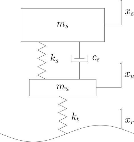
To illustrate the limit filter and smoother we present an automotive application. The problem considered is to construct both in real time and offline an accurate map of a road profile without the use of optical sensors (e.g. profilometer). Road profile measurement (estimation) is important for vehicle dynamics studies and vehicle development, driver training, and for road surface quality monitoring, which motivates the exploration of methods which do not require sophisticated sensing and instrumentation. In our example, a vehicle is assumed to be equipped with a global positioning system (GPS) sensor and basic suspension sensors. We consider the standard quarter-car suspension model of Figure 1 with dynamical equations: $\begin{array}{rl}{m}_s{\ddot{x}}_s& =-k_s(x_s-x_u)-c_s({\dot{x}}_s-{\dot{x}}_u),\\ m_u{\ddot{x}}_u& =k_s(x_s-x_u)+c_s({\dot{x}}_s-{\dot{x}}_u)-k_t(x_u-x_r)\end{array}$where $m_s$ and $m_u$ are sprung and unsprung masses, $k_s$ and $c_s$ are suspension spring and damper constants and $k_t$ is a tyre stiffness constant, and the coordinates $x_s$, $x_u$ and $x_r$ represent displacements of $m_s$, $m_u$ and road respectively. The road profile $x_r$ is treated as an unknown system input. We begin by considering a sensor set consisting of accelerometers located on $m_s$ and $m_u$, a suspension deflection sensor, and a GPS sensor located on $m_s$ that measures $x_s$. We, therefore, select the state, input and measurement vectors as follows: $x=:\left[\begin{array}{c}{x}_s\\ {\dot{x}}_s\\ x_u\\ {\dot{x}}_u\end{array}\right],w=:\left[\begin{array}{c}{x}_r\end{array}\right],z=:\left[\begin{array}{c}{x}_s\\ x_s-x_u\\ {\ddot{x}}_s\\ {\ddot{x}}_u\end{array}\right].$The model is discretised using Euler's method with a time-step $\mathrm{\Delta }t$ to give the state-space equations (1(1) $\begin{array}{rl}{x}_{k+1}& =A{x}_k+B{w}_k,\end{array}$(1) )–(2(2) $\begin{array}{rl}{z}_k& =C{x}_k+D{w}_k+v_k\end{array}$(2) ) with system matrices: $\begin{array}{rl}A& =\left[\begin{array}{cccc}1& \mathrm{\Delta }t& 0& 0\\ -{\displaystyle \frac{k_s}{m_s}}\mathrm{\Delta }t& 1-{\displaystyle \frac{c_s}{m_s}}\mathrm{\Delta }t& {\displaystyle \frac{k_s}{m_s}}\mathrm{\Delta }t& {\displaystyle \frac{c_s}{m_s}}\mathrm{\Delta }t\\ 0& 0& 1& \mathrm{\Delta }t\\ {\displaystyle \frac{k_s}{m_u}}\mathrm{\Delta }t& {\displaystyle \frac{c_s}{m_u}}\mathrm{\Delta }t& -{\displaystyle \frac{k_s+k_t}{m_u}}\mathrm{\Delta }t& 1-{\displaystyle \frac{c_s}{m_u}}\mathrm{\Delta }t\end{array}\right],\\ B& =\left[\begin{array}{c}0\\ 0\\ 0\\ {\displaystyle \frac{k_t}{m_u}}\mathrm{\Delta }t\end{array}\right],\\ C& =\left[\begin{array}{cccc}1& 0& 0& 0\\ 1& 0& -1& 0\\ -{\displaystyle \frac{k_s}{m_s}}& -{\displaystyle \frac{c_s}{m_s}}& {\displaystyle \frac{k_s}{m_s}}& {\displaystyle \frac{c_s}{m_s}}\\ {\displaystyle \frac{k_s}{m_u}}& {\displaystyle \frac{c_s}{m_u}}& -{\displaystyle \frac{k_s+k_t}{m_u}}& -{\displaystyle \frac{c_s}{m_u}}\end{array}\right],D=\left[\begin{array}{c}0\\ 0\\ 0\\ {\displaystyle \frac{k_t}{m_u}}\end{array}\right].\end{array}$

Figure 1. Quarter vehicle suspension model.

6.2. Convergence and stability of the limit filter

We now investigate the convergence properties of the limit filter. Among the measurements in z it is the measurement of ${\ddot{x}}_u$ (namely the use of an unsprung mass accelerometer sensor) which ensures that D is full column rank. We now consider the system matrix of Lemma 5.4: (44) $\begin{array}{rl}& [\begin{array}{cc}1-z& \mathrm{\Delta }t\\ -{\displaystyle \frac{k_s\mathrm{\Delta }t}{m_s}}& 1-z-{\displaystyle \frac{c_s\mathrm{\Delta }t}{m_s}}\\ 0& 0\\ {\displaystyle \frac{k_s\mathrm{\Delta }t}{m_u}}& {\displaystyle \frac{c_s\mathrm{\Delta }t}{m_u}}\\ 1& 0\\ 1& 0\\ -{\displaystyle \frac{k_s}{m_s}}& -{\displaystyle \frac{c_s}{m_s}}\\ {\displaystyle \frac{k_s}{m_u}}& {\displaystyle \frac{c_s}{m_u}}\end{array}\\ & \begin{array}{ccc}0& 0& 0\\ {\displaystyle \frac{k_s\mathrm{\Delta }t}{m_s}}& {\displaystyle \frac{c_s\mathrm{\Delta }t}{m_s}}& 0\\ 1-z& \mathrm{\Delta }t& 0\\ -{\displaystyle \frac{(k_s+k_t)\mathrm{\Delta }t}{m_u}}& 1-z-{\displaystyle \frac{c_s\mathrm{\Delta }t}{m_u}}& {\displaystyle \frac{k_t\mathrm{\Delta }t}{m_u}}\\ 0& 0& 0\\ -1& 0& 0\\ {\displaystyle \frac{k_s}{m_s}}& {\displaystyle \frac{c_s}{m_s}}& 0\\ -{\displaystyle \frac{(k_s+k_t)}{m_u}}& -{\displaystyle \frac{c_s}{m_u}}& {\displaystyle \frac{k_t}{m_u}}\end{array}]\end{array}$(44) and investigate if there are any values of z where it loses rank. Denoting by ${\rho }_n$ the nth row of (44(44) $\begin{array}{rl}& [\begin{array}{cc}1-z& \mathrm{\Delta }t\\ -{\displaystyle \frac{k_s\mathrm{\Delta }t}{m_s}}& 1-z-{\displaystyle \frac{c_s\mathrm{\Delta }t}{m_s}}\\ 0& 0\\ {\displaystyle \frac{k_s\mathrm{\Delta }t}{m_u}}& {\displaystyle \frac{c_s\mathrm{\Delta }t}{m_u}}\\ 1& 0\\ 1& 0\\ -{\displaystyle \frac{k_s}{m_s}}& -{\displaystyle \frac{c_s}{m_s}}\\ {\displaystyle \frac{k_s}{m_u}}& {\displaystyle \frac{c_s}{m_u}}\end{array}\\ & \begin{array}{ccc}0& 0& 0\\ {\displaystyle \frac{k_s\mathrm{\Delta }t}{m_s}}& {\displaystyle \frac{c_s\mathrm{\Delta }t}{m_s}}& 0\\ 1-z& \mathrm{\Delta }t& 0\\ -{\displaystyle \frac{(k_s+k_t)\mathrm{\Delta }t}{m_u}}& 1-z-{\displaystyle \frac{c_s\mathrm{\Delta }t}{m_u}}& {\displaystyle \frac{k_t\mathrm{\Delta }t}{m_u}}\\ 0& 0& 0\\ -1& 0& 0\\ {\displaystyle \frac{k_s}{m_s}}& {\displaystyle \frac{c_s}{m_s}}& 0\\ -{\displaystyle \frac{(k_s+k_t)}{m_u}}& -{\displaystyle \frac{c_s}{m_u}}& {\displaystyle \frac{k_t}{m_u}}\end{array}]\end{array}$(44) ) and noting that elementary row operations preserve rank, we perform sequentially the following operations: $\begin{array}{rl}{\rho }_1& \to \mathrm{\Delta }{t}^{-1}({\rho }_1-(1-z){\rho }_5),\\ {\rho }_6& \to -{\rho }_6+{\rho }_5,\\ {\rho }_3& \to \mathrm{\Delta }{t}^{-1}({\rho }_3-(1-z){\rho }_6),\\ {\rho }_8& \to m_u{\rho }_8-k_s{\rho }_5+(k_s+k_t){\rho }_6-c_s({\rho }_1-{\rho }_3)\end{array}$followed by reordering and rescaling to obtain a matrix whose first five rows are the identity matrix, which is obviously full column rank for all z. In a similar way, we can show that the matrix $[A-zI,B]$ (first 4 rows of (44(44) $\begin{array}{rl}& [\begin{array}{cc}1-z& \mathrm{\Delta }t\\ -{\displaystyle \frac{k_s\mathrm{\Delta }t}{m_s}}& 1-z-{\displaystyle \frac{c_s\mathrm{\Delta }t}{m_s}}\\ 0& 0\\ {\displaystyle \frac{k_s\mathrm{\Delta }t}{m_u}}& {\displaystyle \frac{c_s\mathrm{\Delta }t}{m_u}}\\ 1& 0\\ 1& 0\\ -{\displaystyle \frac{k_s}{m_s}}& -{\displaystyle \frac{c_s}{m_s}}\\ {\displaystyle \frac{k_s}{m_u}}& {\displaystyle \frac{c_s}{m_u}}\end{array}\\ & \begin{array}{ccc}0& 0& 0\\ {\displaystyle \frac{k_s\mathrm{\Delta }t}{m_s}}& {\displaystyle \frac{c_s\mathrm{\Delta }t}{m_s}}& 0\\ 1-z& \mathrm{\Delta }t& 0\\ -{\displaystyle \frac{(k_s+k_t)\mathrm{\Delta }t}{m_u}}& 1-z-{\displaystyle \frac{c_s\mathrm{\Delta }t}{m_u}}& {\displaystyle \frac{k_t\mathrm{\Delta }t}{m_u}}\\ 0& 0& 0\\ -1& 0& 0\\ {\displaystyle \frac{k_s}{m_s}}& {\displaystyle \frac{c_s}{m_s}}& 0\\ -{\displaystyle \frac{(k_s+k_t)}{m_u}}& -{\displaystyle \frac{c_s}{m_u}}& {\displaystyle \frac{k_t}{m_u}}\end{array}]\end{array}$(44) )) has full row rank for all z, hence $(A,B)$ is controllable. It, therefore, follows that the stability and convergence results of Lemma 5.1, 5.2 and Theorem 5.5 hold. It can be verified that the condition of Lemma 5.4 holds even without measurement of $x_s-x_u$ (suspension deflection) and ${\ddot{x}}_s$ (sprung mass acceleration). However, the condition fails if the measurement of $x_s$ (GPS sensor) is removed. The condition on $(A,B)$ does not change if any of the measurements are removed.

A similar analysis to the above can be carried out for other choices of sensors. For example, a profilometer which measures $x_s-x_r$ could be considered. In this case, another non-zero entry appears in the D matrix. Thus the profilometer could be considered as an alternative to the measurement of ${\ddot{x}}_u$ to ensure that D is full rank. Similar conclusions hold in this case, namely, the required detectability holds if $x_s$ is measured but not if only measurements of ${\ddot{x}}_u$ and $x_s-x_r$ are available.

6.3. Simulation results and discussion

We apply the limit filter and smoother of Theorems 3.2 and 4.2 with an additional requirement that the GPS sampling period is longer than the time-step $\mathrm{\Delta }t$. Hence, the measurement vector is time varying with the row corresponding to the GPS replaced by zeros unless a GPS measurement is available. The filter and smoother recursions remain the same with the system matrices replaced by their time-varying counterparts. We demonstrate the performance of the filter and smoother on simulated data with a road profile (specified for convenience as a function of time) that consists of a square wave (period 0.5 s, amplitude 0.2 m), followed by a downward ramp (slope $-1$ m/s) and finally a Brownian motion (integrated white noise of standard deviation 0.05 m for the discretisation length $\mathrm{\Delta }t$). The vehicle model parameters are $m_s=350$ kg, $m_u=50$ kg, $k_s=20$ kN/m, $c_s=1$ kNs/m, $k_t=200$ kN/m and the discretisation length is $\mathrm{\Delta }t=1$ ms. The GPS measurements are available in regular intervals of 1 second. Simulated white noise with standard deviation as in Table 1 is added to the four measurements to generate the vector $z_k$ that is input to the limit filter, with standard deviations chosen to reflect the different accuracies expected from the sensors.

Table 1. Sensor noise parameters.

Sensor	Standard deviation of noise
GPS	1 m
Suspension deflection	0.01 m
Accelerometer	0.1 m/s${}^2$

The same model parameters are used for the limit filter and smoother, and the measurement error covariance matrix is taken to be: $R=\text{diag}\{1,{10}^{-4},{10}^{-2},{10}^{-2}\}$. The initial state covariance is set to ${\overline{P}}_{0|-1}=\text{diag}\{1,{10}^{-2},1,{10}^{-2}\}$ and the filter sprung and unsprung mass position states are initialised with an error of 2 m (equal to 2 standard deviations). The true, filtered and smoothed sprung and unsprung mass position states and road profile are plotted in Figure 2 with the shaded regions representing the 1 standard deviation confidence intervals.

Figure 2. True, filtered and smoothed sprung and unsprung mass position states and road profile input.

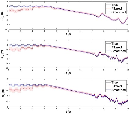
It is observed that the filter reduces the large initialisation error over time and that the smoother improves on the filtered estimates over the entire simulation interval and especially at the start. The standard deviation of the smoothed estimates is smaller (or equal) than that of the filtered estimates (see Remark 4.2) and the difference is also most pronounced at the start of the simulation interval. Further note that the smoother generates a realistic state trajectory, which is because the smoothed state and input trajectories, unlike the filtered trajectories, satisfy the model dynamics (see Remark 4.1). Lastly, note that the limit filter is able to blend the different measurements to achieve good performance in contrasting situations. For example, rapid changes in $x_r$ are dealt with as well as slow drift. This is similar to the property in localisation/tracking filters that integrate inertial measurement unit (IMU) and GPS sensors to estimate a system state, whereas here the limit filter is used to estimate an unknown system input (road profile). Note also that we have avoided the difficulty with the standard Kalman filter (3(3) $\begin{array}{rl}{\hat{x}}_{k|k}& ={\hat{x}}_{k|k-1}+K_{x,k}(z_k-C{\hat{x}}_{k|k-1}),\end{array}$(3) )–(12(12) $\begin{array}{rl}{P}_{k+1|k}& =\left[AB\right]\left[\begin{array}{cc}{P}_{k|k}& P_{k|k}^{xw}\\ P_{k|k}^{wx}& P_{k|k}^{ww}\end{array}\right]{\left[AB\right]}^T.\end{array}$(12) ) of specifying a suitable mean and covariance for the exogenous input.

7. Conclusion

This paper has derived two forms for the zero informational limit of the Kalman filter with feedthrough of the process noise to the measurements. We have shown that the recursions in the first form are closely related to those of Gillijns and De Moor (2007b) and hence we have provided an alternative interpretation for that recursive filter. The second form takes the form of the standard Kalman filter for a modified system (Theorem 3.2). This form is convenient to derive conditions for the asymptotic convergence of the limit filter to steady state form which can be conveniently expressed in terms of the original system matrices as a minimum phase and a controllability condition (Theorem 5.5). We further derive the fixed interval Kalman smoother with feedthrough of the process noise to the measurements (Theorem 4.1) and then find the zero informational limit with respect to the process noise (Theorem 4.2). Both the filter and smoother are applied successfully to a quarter-car model to accurately map road elevation using a GPS and vehicle suspension sensors in simulation.

An interesting question for future work is to ask if a stochastic filtering and smoothing problem can be posed and solved directly for a completely unknown exogenous input (without process noise) and whether the solution coincides with the limit filter and smoother of the present paper. In turn, it would be interesting to compare this with the problem of the limiting form of the Kalman filter when the measurement noise covariance tends to zero and the related singular filtering problem (Moylan, 1974; Shaked, 1985).

Acknowledgments

The first author would like to acknowledge McLaren Automotive Ltd for a CASE studentship awarded for doctoral research.

Additional information

Funding

This work was supported by McLaren Automotive Ltd.

Appendices

Appendix 1. Proof of Theorem 3.1

For convenience, we state the matrix inversion lemma (see Anderson & Moore, 2012, Sec. 6.3) which is used in the proof.

Lemma A.1

Let $S=S^T>0$, $T=T^T>0$ and H be arbitrary of compatible dimension. Then: (A1) $\begin{array}{rl}& S-S{H}^T(HS{H}^T+T{)}^{-1}HS=(S^{-1}+H^T{T}^{-1}H{)}^{-1},\end{array}$(A1) (A2) $\begin{array}{rl}& S{H}^T(HS{H}^T+T{)}^{-1}=(S^{-1}+H^T{T}^{-1}H{)}^{-1}{H}^T{T}^{-1}.\end{array}$(A2)

To prove Theorem 3.1 we will proceed inductively, first considering the recursive expressions (3(3) $\begin{array}{rl}{\hat{x}}_{k|k}& ={\hat{x}}_{k|k-1}+K_{x,k}(z_k-C{\hat{x}}_{k|k-1}),\end{array}$(3) )–(12(12) $\begin{array}{rl}{P}_{k+1|k}& =\left[AB\right]\left[\begin{array}{cc}{P}_{k|k}& P_{k|k}^{xw}\\ P_{k|k}^{wx}& P_{k|k}^{ww}\end{array}\right]{\left[AB\right]}^T.\end{array}$(12) ) in the limit as $Q^{-1}\to 0$. Suppose for a given k, ${\hat{x}}_{k|k-1}(Q)$ and $P_{k|k-1}(Q)$ tend to well-defined limits ${\overline{x}}_{k|k-1}$ and ${\overline{P}}_{k|k-1}(Q)$ as $Q^{-1}\to 0$. We will show that ${\hat{x}}_{k|k}(Q)$, ${\hat{w}}_{k|k}(Q)$, $P_{k|k}(Q)$, $P_{k|k}^{ww}(Q)$, $P_{k|k}^{xw}(Q)$, ${\hat{x}}_{k+1|k}(Q)$, $P_{k+1|k}(Q)$ have well-defined limits given by (13(13) $\begin{array}{rl}{\overline{x}}_{k|k}& ={\overline{x}}_{k|k-1}+L_{x,k}(z_k-C{\overline{x}}_{k|k-1}-D{\overline{w}}_{k|k}),\end{array}$(13) )–(22(22) $\begin{array}{rl}{\overline{P}}_{k+1|k}& =\left[AB\right]\left[\begin{array}{cc}{\overline{P}}_{k|k}& {\overline{P}}_{k|k}^{xw}\\ {\overline{P}}_{k|k}^{wx}& {\overline{P}}_{k|k}^{ww}\end{array}\right]{\left[AB\right]}^T\end{array}$(22) ). Substituting for ${\mathrm{\Theta }}_k$ from (10(10) $\begin{array}{rl}{\mathrm{\Theta }}_k& =C{P}_{k|k-1}{C}^T+DQ{D}^T+R\end{array}$(10) ) into (9(9) $\begin{array}{rl}{K}_{w,k}& =Q{D}^T{\mathrm{\Theta }}_k^{-1},\end{array}$(9) ) and using (A2(A2) $\begin{array}{rl}& S{H}^T(HS{H}^T+T{)}^{-1}=(S^{-1}+H^T{T}^{-1}H{)}^{-1}{H}^T{T}^{-1}.\end{array}$(A2) ) gives: (A3) $K_{w,k}=(Q^{-1}+D^T{\mathrm{\Sigma }}_k^{-1}D{)}^{-1}{D}^T{\mathrm{\Sigma }}_k^{-1}$(A3) where: ${\mathrm{\Sigma }}_k=C{P}_{k|k-1}(Q)C^T+R.$Taking the limit as $Q^{-1}\to 0$ in (A3(A3) $K_{w,k}=(Q^{-1}+D^T{\mathrm{\Sigma }}_k^{-1}D{)}^{-1}{D}^T{\mathrm{\Sigma }}_k^{-1}$(A3) ), $K_{w,k}$ approaches $L_{w,k}$, where ${\overline{\mathrm{\Sigma }}}_k$ is defined in (20(20) $\begin{array}{rl}{\overline{\mathrm{\Sigma }}}_k& =C{\overline{P}}_{k|k-1}{C}^T+R\end{array}$(20) ). It follows that (4(4) $\begin{array}{rl}{\hat{w}}_{k|k}& =K_{w,k}(z_k-C{\hat{x}}_{k|k-1}),\end{array}$(4) ) has a well-defined limit given by (14(14) $\begin{array}{rl}{\overline{w}}_{k|k}& =L_{w,k}(z_k-C{\overline{x}}_{k|k-1}),\end{array}$(14) ). Now substitute for $K_{x,k}$ in (7(7) $\begin{array}{rl}{P}_{k|k}^{xw}& =(P_{k|k}^{wx}{)}^T=-K_{x,k}{\mathrm{\Theta }}_k{K}_{w,k}^T,\end{array}$(7) ) and let $L_{x,k}$ be defined as in (18(18) $\begin{array}{rl}{L}_{x,k}& ={\overline{P}}_{k|k-1}{C}^T{\overline{\mathrm{\Sigma }}}_k^{-1},\end{array}$(18) ). Then (7(7) $\begin{array}{rl}{P}_{k|k}^{xw}& =(P_{k|k}^{wx}{)}^T=-K_{x,k}{\mathrm{\Theta }}_k{K}_{w,k}^T,\end{array}$(7) ) has a well-defined limit given by (17(17) $\begin{array}{rl}{\overline{P}}_{k|k}^{xw}& =-L_{x,k}{\overline{\mathrm{\Sigma }}}_k{L}_{w,k}^T,\end{array}$(17) ). Applying (A1(A1) $\begin{array}{rl}& S-S{H}^T(HS{H}^T+T{)}^{-1}HS=(S^{-1}+H^T{T}^{-1}H{)}^{-1},\end{array}$(A1) ) to (10(10) $\begin{array}{rl}{\mathrm{\Theta }}_k& =C{P}_{k|k-1}{C}^T+DQ{D}^T+R\end{array}$(10) ) gives: (A4) ${\mathrm{\Theta }}_k^{-1}={\mathrm{\Sigma }}_k^{-1}-{\mathrm{\Sigma }}_k^{-1}D(D^T{\mathrm{\Sigma }}_k^{-1}D+Q^{-1}{)}^{-1}{D}^T{\mathrm{\Sigma }}_k^{-1}.$(A4) Substituting for (8(8) $\begin{array}{rl}{K}_{x,k}& =P_{k|k-1}{C}^T{\mathrm{\Theta }}_k^{-1},\end{array}$(8) ) and then (A4(A4) ${\mathrm{\Theta }}_k^{-1}={\mathrm{\Sigma }}_k^{-1}-{\mathrm{\Sigma }}_k^{-1}D(D^T{\mathrm{\Sigma }}_k^{-1}D+Q^{-1}{)}^{-1}{D}^T{\mathrm{\Sigma }}_k^{-1}.$(A4) ) into (3(3) $\begin{array}{rl}{\hat{x}}_{k|k}& ={\hat{x}}_{k|k-1}+K_{x,k}(z_k-C{\hat{x}}_{k|k-1}),\end{array}$(3) ) and taking the limit as $Q^{-1}\to 0$, ${\hat{x}}_{k|k}$ has a well-defined limit given by: (A5) $\begin{array}{rl}{\overline{x}}_{k|k}& ={\overline{x}}_{k|k-1}+{\overline{P}}_{k|k-1}{C}^T{\overline{\mathrm{\Sigma }}}_k^{-1}(I-D(D^T{\overline{\mathrm{\Sigma }}}_k^{-1}D{)}^{-1}{D}^T{\overline{\mathrm{\Sigma }}}_k^{-1})\\ & \times (z_k-C{\overline{x}}_{k|k-1}).\end{array}$(A5) Making use of the expressions for ${\overline{w}}_{k|k}$ and $L_{x,k}$ in (A5(A5) $\begin{array}{rl}{\overline{x}}_{k|k}& ={\overline{x}}_{k|k-1}+{\overline{P}}_{k|k-1}{C}^T{\overline{\mathrm{\Sigma }}}_k^{-1}(I-D(D^T{\overline{\mathrm{\Sigma }}}_k^{-1}D{)}^{-1}{D}^T{\overline{\mathrm{\Sigma }}}_k^{-1})\\ & \times (z_k-C{\overline{x}}_{k|k-1}).\end{array}$(A5) ) gives (13(13) $\begin{array}{rl}{\overline{x}}_{k|k}& ={\overline{x}}_{k|k-1}+L_{x,k}(z_k-C{\overline{x}}_{k|k-1}-D{\overline{w}}_{k|k}),\end{array}$(13) ). Substituting for $K_{w,k}$ from (9(9) $\begin{array}{rl}{K}_{w,k}& =Q{D}^T{\mathrm{\Theta }}_k^{-1},\end{array}$(9) ) and ${\mathrm{\Theta }}_k$ from (10(10) $\begin{array}{rl}{\mathrm{\Theta }}_k& =C{P}_{k|k-1}{C}^T+DQ{D}^T+R\end{array}$(10) ) into (6(6) $\begin{array}{rl}{P}_{k|k}^{ww}& =Q-K_{w,k}{\mathrm{\Theta }}_k{K}_{w,k}^T,\end{array}$(6) ) and applying (A1(A1) $\begin{array}{rl}& S-S{H}^T(HS{H}^T+T{)}^{-1}HS=(S^{-1}+H^T{T}^{-1}H{)}^{-1},\end{array}$(A1) ) gives: $P_{k|k}^{ww}=(Q^{-1}+D^T{\mathrm{\Sigma }}_k^{-1}D{)}^{-1}.$Taking the limit as $Q^{-1}\to 0$, $P_{k|k}^{ww}$ has a well-defined limit given by: (A6) ${\overline{P}}_{k|k}^{ww}=(D^T{\overline{\mathrm{\Sigma }}}_k^{-1}D{)}^{-1}.$(A6) This expression can be equivalently written in terms of $L_{w,k}$ in the form (16(16) $\begin{array}{rl}{\overline{P}}_{k|k}^{ww}& =L_{w,k}{\overline{\mathrm{\Sigma }}}_k{L}_{w,k}^T,\end{array}$(16) ). Substituting for $K_{x,k}$ from (8(8) $\begin{array}{rl}{K}_{x,k}& =P_{k|k-1}{C}^T{\mathrm{\Theta }}_k^{-1},\end{array}$(8) ) and ${\mathrm{\Theta }}_k^{-1}$ from (A4(A4) ${\mathrm{\Theta }}_k^{-1}={\mathrm{\Sigma }}_k^{-1}-{\mathrm{\Sigma }}_k^{-1}D(D^T{\mathrm{\Sigma }}_k^{-1}D+Q^{-1}{)}^{-1}{D}^T{\mathrm{\Sigma }}_k^{-1}.$(A4) ) into (5(5) $\begin{array}{rl}{P}_{k|k}& =P_{k|k-1}-K_{x,k}{\mathrm{\Theta }}_k{K}_{x,k}^T,\end{array}$(5) ), taking the limit as $Q^{-1}\to 0$, and then using the expressions for $L_{x,k}$ and ${\overline{P}}_{k|k}^{ww}$ from (A6(A6) ${\overline{P}}_{k|k}^{ww}=(D^T{\overline{\mathrm{\Sigma }}}_k^{-1}D{)}^{-1}.$(A6) ), $P_{k|k}$ has a well-defined limit given by (15(15) $\begin{array}{rl}{\overline{P}}_{k|k}& ={\overline{P}}_{k|k-1}-L_{x,k}({\overline{\mathrm{\Sigma }}}_k-D{\overline{P}}_{k|k}^{ww}{D}^T)L_{x,k}^T,\end{array}$(15) ). Taking the limit as $Q^{-1}\to 0$ in (11(11) $\begin{array}{rl}{\hat{x}}_{k+1|k}& =\left[AB\right]\left[\begin{array}{c}{\hat{x}}_{k|k}\\ {\hat{w}}_{k|k}\end{array}\right],\end{array}$(11) ) and (12(12) $\begin{array}{rl}{P}_{k+1|k}& =\left[AB\right]\left[\begin{array}{cc}{P}_{k|k}& P_{k|k}^{xw}\\ P_{k|k}^{wx}& P_{k|k}^{ww}\end{array}\right]{\left[AB\right]}^T.\end{array}$(12) ), ${\hat{x}}_{k+1|k}$ and $P_{k+1|k}$ have well-defined limits given by (21(21) $\begin{array}{rl}{\overline{x}}_{k+1|k}& =\left[AB\right]\left[\begin{array}{c}{\overline{x}}_{k|k}\\ {\overline{w}}_{k|k}\end{array}\right],\end{array}$(21) ) and (22(22) $\begin{array}{rl}{\overline{P}}_{k+1|k}& =\left[AB\right]\left[\begin{array}{cc}{\overline{P}}_{k|k}& {\overline{P}}_{k|k}^{xw}\\ {\overline{P}}_{k|k}^{wx}& {\overline{P}}_{k|k}^{ww}\end{array}\right]{\left[AB\right]}^T\end{array}$(22) ) respectively. The result follows by induction since, by definition, ${\overline{x}}_{0|-1}={\hat{x}}_{0|-1}=\underset{Q^{-1}\to 0}{lim}{\hat{x}}_{0|-1}$ and ${\overline{P}}_{0|-1}=P_{0|-1}=\underset{Q^{-1}\to 0}{lim}{P}_{0|-1}$.

Appendix 2

Proof of Theorem 3.2

We first establish the following lemma.

Lemma A.2

Suppose D has full column rank, $R=R^T>0$ and $S=S^T\ge 0$ of appropriate dimensions, then: (A7) $\begin{array}{rl}& (S+R{)}^{-1}-(S+R{)}^{-1}D(D^T(S+R{)}^{-1}D{)}^{-1}{D}^T(S+R{)}^{-1}\\ & =(I-\mathrm{\Pi }{)}^T((I-\mathrm{\Pi })S(I-\mathrm{\Pi }{)}^T+R{)}^{-1}(I-\mathrm{\Pi })\end{array}$(A7) where $\mathrm{\Pi }=D(D^T{R}^{-1}D{)}^{-1}{D}^T{R}^{-1}$ as in (33(33) $\begin{array}{rl}\mathrm{\Pi }& =D{D}^{†},\end{array}$(33) ).

Proof.

We first introduce the projection: (A8) ${\mathrm{\Pi }}_S=D(D^T(S+R{)}^{-1}D{)}^{-1}{D}^T(S+R{)}^{-1}.$(A8) We observe that Π and ${\mathrm{\Pi }}_S$ are parallel projections onto the same space, namely the column space of D, but have different null spaces. Further note that ${\mathrm{\Pi }}^2={\mathrm{\Pi }}_S\mathrm{\Pi }=\mathrm{\Pi }$, ${\mathrm{\Pi }}_S^2=\mathrm{\Pi }{\mathrm{\Pi }}_S={\mathrm{\Pi }}_S$ and: (A9) $\begin{array}{rl}& (I-\mathrm{\Pi }){\mathrm{\Pi }}_S=0,\end{array}$(A9) (A10) $\begin{array}{rl}& (I-{\mathrm{\Pi }}_S)\mathrm{\Pi }=0,\end{array}$(A10) (A11) $\begin{array}{rl}& {\mathrm{\Pi }}_S^T{R}^{-1}(I-\mathrm{\Pi })=0,\end{array}$(A11) (A12) $\begin{array}{rl}& {\mathrm{\Pi }}^T(S+R{)}^{-1}(I-{\mathrm{\Pi }}_S)=0.\end{array}$(A12) We first claim that: (A13) $((I-\mathrm{\Pi })S(I-\mathrm{\Pi }{)}^T+R{)}^{-1}(I-\mathrm{\Pi })=(S+R{)}^{-1}(I-{\mathrm{\Pi }}_S).$(A13) To see this note that: $(I-\mathrm{\Pi })S(I-\mathrm{\Pi }{)}^T+R=(I-\mathrm{\Pi })(S+R)+(R-(I-\mathrm{\Pi })S){\mathrm{\Pi }}^T$using $\mathrm{\Pi }R=R{\mathrm{\Pi }}^T$. Therefore using (A9(A9) $\begin{array}{rl}& (I-\mathrm{\Pi }){\mathrm{\Pi }}_S=0,\end{array}$(A9) ) and (A12(A12) $\begin{array}{rl}& {\mathrm{\Pi }}^T(S+R{)}^{-1}(I-{\mathrm{\Pi }}_S)=0.\end{array}$(A12) ): $\begin{array}{rl}& ((I-\mathrm{\Pi })S(I-\mathrm{\Pi }{)}^T+R)(S+R{)}^{-1}(I-{\mathrm{\Pi }}_S)\\ & =(I-\mathrm{\Pi })(I-{\mathrm{\Pi }}_S)+(R-(I-\mathrm{\Pi })S){\mathrm{\Pi }}^T(S+R{)}^{-1}(I-{\mathrm{\Pi }}_S)\\ & =(I-\mathrm{\Pi })\end{array}$from which (A13(A13) $((I-\mathrm{\Pi })S(I-\mathrm{\Pi }{)}^T+R{)}^{-1}(I-\mathrm{\Pi })=(S+R{)}^{-1}(I-{\mathrm{\Pi }}_S).$(A13) ) follows. Further from (A12(A12) $\begin{array}{rl}& {\mathrm{\Pi }}^T(S+R{)}^{-1}(I-{\mathrm{\Pi }}_S)=0.\end{array}$(A12) ) and (A13(A13) $((I-\mathrm{\Pi })S(I-\mathrm{\Pi }{)}^T+R{)}^{-1}(I-\mathrm{\Pi })=(S+R{)}^{-1}(I-{\mathrm{\Pi }}_S).$(A13) ): (A14) ${\mathrm{\Pi }}^T((I-\mathrm{\Pi })S(I-\mathrm{\Pi }{)}^T+R{)}^{-1}(I-\mathrm{\Pi })=0.$(A14) Hence, substituting ${\mathrm{\Pi }}_S$ from (A8(A8) ${\mathrm{\Pi }}_S=D(D^T(S+R{)}^{-1}D{)}^{-1}{D}^T(S+R{)}^{-1}.$(A8) ) into (A13(A13) $((I-\mathrm{\Pi })S(I-\mathrm{\Pi }{)}^T+R{)}^{-1}(I-\mathrm{\Pi })=(S+R{)}^{-1}(I-{\mathrm{\Pi }}_S).$(A13) ) gives (A7(A7) $\begin{array}{rl}& (S+R{)}^{-1}-(S+R{)}^{-1}D(D^T(S+R{)}^{-1}D{)}^{-1}{D}^T(S+R{)}^{-1}\\ & =(I-\mathrm{\Pi }{)}^T((I-\mathrm{\Pi })S(I-\mathrm{\Pi }{)}^T+R{)}^{-1}(I-\mathrm{\Pi })\end{array}$(A7) ).

We next establish several identities that are needed in the proof.

1. We claim that: (A15) ${\overline{K}}_k=L_{x,k}(I-D{L}_{w,k}).$(A15) To see this note that on substitution from (18(18) $\begin{array}{rl}{L}_{x,k}& ={\overline{P}}_{k|k-1}{C}^T{\overline{\mathrm{\Sigma }}}_k^{-1},\end{array}$(18) ) and (19(19) $\begin{array}{rl}{L}_{w,k}& =(D^T{\overline{\mathrm{\Sigma }}}_k^{-1}D{)}^{-1}{D}^T{\overline{\mathrm{\Sigma }}}_k^{-1},\end{array}$(19) ) the right hand side of (A15(A15) ${\overline{K}}_k=L_{x,k}(I-D{L}_{w,k}).$(A15) ) becomes: ${\overline{P}}_{k|k-1}{C}^T({\overline{\mathrm{\Sigma }}}_k^{-1}-{\overline{\mathrm{\Sigma }}}_k^{-1}D(D^T{\overline{\mathrm{\Sigma }}}_k^{-1}D{)}^{-1}{D}^T{\overline{\mathrm{\Sigma }}}_k^{-1})$which equals: (A16) ${\overline{P}}_{k|k-1}{C}^T((I-\mathrm{\Pi }{)}^T((I-\mathrm{\Pi })S(I-\mathrm{\Pi }{)}^T+R{)}^{-1}(I-\mathrm{\Pi }))$(A16) after applying (A7(A7) $\begin{array}{rl}& (S+R{)}^{-1}-(S+R{)}^{-1}D(D^T(S+R{)}^{-1}D{)}^{-1}{D}^T(S+R{)}^{-1}\\ & =(I-\mathrm{\Pi }{)}^T((I-\mathrm{\Pi })S(I-\mathrm{\Pi }{)}^T+R{)}^{-1}(I-\mathrm{\Pi })\end{array}$(A7) ) with $S=C{\overline{P}}_{k|k-1}{C}^T$ and noting that ${\overline{\mathrm{\Sigma }}}_k=S+R$ from (20(20) $\begin{array}{rl}{\overline{\mathrm{\Sigma }}}_k& =C{\overline{P}}_{k|k-1}{C}^T+R\end{array}$(20) ). Using the transpose of (A14(A14) ${\mathrm{\Pi }}^T((I-\mathrm{\Pi })S(I-\mathrm{\Pi }{)}^T+R{)}^{-1}(I-\mathrm{\Pi })=0.$(A14) ), the $I-\mathrm{\Pi }$ on the right in (A16(A16) ${\overline{P}}_{k|k-1}{C}^T((I-\mathrm{\Pi }{)}^T((I-\mathrm{\Pi })S(I-\mathrm{\Pi }{)}^T+R{)}^{-1}(I-\mathrm{\Pi }))$(A16) ) can be removed, which gives (35(35) $\begin{array}{rl}{\overline{K}}_k& ={\overline{P}}_{k|k-1}{C}_1^T(C_1{\overline{P}}_{k|k-1}{C}_1^T+R{)}^{-1}.\end{array}$(35) ) on substituting from (32(32) $\begin{array}{rl}{C}_1& =(I-\mathrm{\Pi })C,\end{array}$(32) ). This establishes (A15(A15) ${\overline{K}}_k=L_{x,k}(I-D{L}_{w,k}).$(A15) ).

2. From (A15(A15) ${\overline{K}}_k=L_{x,k}(I-D{L}_{w,k}).$(A15) ) it is easy to see that: (A17) ${\overline{K}}_{k}D=0$(A17) since $L_{w,k}D=I$. Hence: (A18) ${\overline{K}}_{k}C={\overline{K}}_k{C}_1.$(A18)

3. We claim that: (A19) ${\overline{K}}_k{C}_1{\overline{P}}_{k|k-1}=L_{x,k}({\overline{\mathrm{\Sigma }}}_k-D{\overline{P}}_{k|k}^{ww}{D}^T)L_{x,k}^T.$(A19) To see this note that on substitution from (18(18) $\begin{array}{rl}{L}_{x,k}& ={\overline{P}}_{k|k-1}{C}^T{\overline{\mathrm{\Sigma }}}_k^{-1},\end{array}$(18) ) and (A6(A6) ${\overline{P}}_{k|k}^{ww}=(D^T{\overline{\mathrm{\Sigma }}}_k^{-1}D{)}^{-1}.$(A6) ) the right hand side of (A19(A19) ${\overline{K}}_k{C}_1{\overline{P}}_{k|k-1}=L_{x,k}({\overline{\mathrm{\Sigma }}}_k-D{\overline{P}}_{k|k}^{ww}{D}^T)L_{x,k}^T.$(A19) ) becomes: $L_{x,k}(I-D(D^T{\overline{\mathrm{\Sigma }}}_k^{-1}D{)}^{-1}{D}^T{\overline{\mathrm{\Sigma }}}_k^{-1})C{\overline{P}}_{k|k-1}$which equals ${\overline{K}}_{k}C{\overline{P}}_{k|k-1}$ using (A15(A15) ${\overline{K}}_k=L_{x,k}(I-D{L}_{w,k}).$(A15) ). Applying (A18(A18) ${\overline{K}}_{k}C={\overline{K}}_k{C}_1.$(A18) ) establishes the claim.

4. We claim that: (A20) $L_{w,k}=D^{†}(I-C{\overline{K}}_k).$(A20) To see this consider: $\begin{array}{rl}{L}_{w,k}-D^{†}(I-C{\overline{K}}_k)& =L_{w,k}-D^{†}+D^{†}C{L}_{x,k}(I-D{L}_{w,k})\\ & =L_{w,k}-D^{†}+D^{†}({\overline{\mathrm{\Sigma }}}_k-R){\overline{\mathrm{\Sigma }}}_k^{-1}(I-D{L}_{w,k})\\ & =-D^{†}R{\overline{\mathrm{\Sigma }}}_k^{-1}(I-D{L}_{w,k})\\ & =-(D^T{R}^{-1}D{)}^{-1}{D}^T{\overline{\mathrm{\Sigma }}}_k^{-1}\\ & \times (I-D(D^T{\overline{\mathrm{\Sigma }}}_k^{-1}D{)}^{-1}{D}^T{\overline{\mathrm{\Sigma }}}_k^{-1})=0\end{array}$ where we have used (A15(A15) ${\overline{K}}_k=L_{x,k}(I-D{L}_{w,k}).$(A15) ), (18(18) $\begin{array}{rl}{L}_{x,k}& ={\overline{P}}_{k|k-1}{C}^T{\overline{\mathrm{\Sigma }}}_k^{-1},\end{array}$(18) ), (20(20) $\begin{array}{rl}{\overline{\mathrm{\Sigma }}}_k& =C{\overline{P}}_{k|k-1}{C}^T+R\end{array}$(20) ), (34(34) $\begin{array}{rl}{D}^{†}& =(D^T{R}^{-1}D{)}^{-1}{D}^T{R}^{-1},\end{array}$(34) ) and (19(19) $\begin{array}{rl}{L}_{w,k}& =(D^T{\overline{\mathrm{\Sigma }}}_k^{-1}D{)}^{-1}{D}^T{\overline{\mathrm{\Sigma }}}_k^{-1},\end{array}$(19) ).

5. To show (27(27) $\begin{array}{rl}{\overline{P}}_{k|k}^{xw}& =-{\overline{P}}_{k|k}(D^{†}C{)}^T\end{array}$(27) ) substitute from (18(18) $\begin{array}{rl}{L}_{x,k}& ={\overline{P}}_{k|k-1}{C}^T{\overline{\mathrm{\Sigma }}}_k^{-1},\end{array}$(18) ) and (A20(A20) $L_{w,k}=D^{†}(I-C{\overline{K}}_k).$(A20) ) into (17(17) $\begin{array}{rl}{\overline{P}}_{k|k}^{xw}& =-L_{x,k}{\overline{\mathrm{\Sigma }}}_k{L}_{w,k}^T,\end{array}$(17) ) and then use (24(24) $\begin{array}{rl}{\overline{P}}_{k|k}& =(I-{\overline{K}}_k{C}_1){\overline{P}}_{k|k-1}\end{array}$(24) ) and (A18(A18) ${\overline{K}}_{k}C={\overline{K}}_k{C}_1.$(A18) ).

6. Lastly, we show (26(26) $\begin{array}{rl}{\overline{P}}_{k|k}^{ww}& =D^{†}(C{\overline{P}}_{k|k}{C}^T+R)(D^{†}{)}^T,\end{array}$(26) ). Substituting (20(20) $\begin{array}{rl}{\overline{\mathrm{\Sigma }}}_k& =C{\overline{P}}_{k|k-1}{C}^T+R\end{array}$(20) ) and (A20(A20) $L_{w,k}=D^{†}(I-C{\overline{K}}_k).$(A20) ) into (16(16) $\begin{array}{rl}{\overline{P}}_{k|k}^{ww}& =L_{w,k}{\overline{\mathrm{\Sigma }}}_k{L}_{w,k}^T,\end{array}$(16) ) gives: (A21) $\begin{array}{rl}{\overline{P}}_{k|k}^{ww}& =D^{†}((I-C{\overline{K}}_k)C{\overline{P}}_{k|k-1}{C}^T+R-C{\overline{K}}_{k}R\\ & -(I-C{\overline{K}}_k){\overline{\mathrm{\Sigma }}}_k(C{\overline{K}}_k{)}^T)(D^{†}{)}^T.\end{array}$(A21) Using (A18(A18) ${\overline{K}}_{k}C={\overline{K}}_k{C}_1.$(A18) ) note that: $\begin{array}{rl}{\overline{\mathrm{\Sigma }}}_k{\overline{K}}_k^T& =(C{\overline{P}}_{k|k-1}{C}_1^T+R){\overline{K}}_k^T,\\ {\overline{K}}_k{\overline{\mathrm{\Sigma }}}_k{\overline{K}}_k^T& ={\overline{K}}_k(C_1{\overline{P}}_{k|k-1}{C}_1^T+R){\overline{K}}_k^T\\ & ={\overline{P}}_{k|k-1}{C}_1^T{\overline{K}}_k^T\end{array}$ from which it follows that: $(I-C{\overline{K}}_k){\overline{\mathrm{\Sigma }}}_k{\overline{K}}_k^T=R{\overline{K}}_k^T.$Noting that $D^{†}R{\overline{K}}_k^T=0$ from (A17(A17) ${\overline{K}}_{k}D=0$(A17) ) the last two terms in (A21(A21) $\begin{array}{rl}{\overline{P}}_{k|k}^{ww}& =D^{†}((I-C{\overline{K}}_k)C{\overline{P}}_{k|k-1}{C}^T+R-C{\overline{K}}_{k}R\\ & -(I-C{\overline{K}}_k){\overline{\mathrm{\Sigma }}}_k(C{\overline{K}}_k{)}^T)(D^{†}{)}^T.\end{array}$(A21) ) are zero. The claim follows using (A18(A18) ${\overline{K}}_{k}C={\overline{K}}_k{C}_1.$(A18) ) and (24(24) $\begin{array}{rl}{\overline{P}}_{k|k}& =(I-{\overline{K}}_k{C}_1){\overline{P}}_{k|k-1}\end{array}$(24) ) on the first term.

Proof of expressions (23(23) $\begin{array}{rl}{\overline{x}}_{k|k}& ={\overline{x}}_{k|k-1}+{\overline{K}}_k(z_k-C_1{\overline{x}}_{k|k-1}),\end{array}$(23) )–(25(25) $\begin{array}{rl}{\overline{w}}_{k|k}& =D^{†}(z_k-C{\overline{x}}_{k|k}),\end{array}$(25) )

Substituting (14(14) $\begin{array}{rl}{\overline{w}}_{k|k}& =L_{w,k}(z_k-C{\overline{x}}_{k|k-1}),\end{array}$(14) ) into (13(13) $\begin{array}{rl}{\overline{x}}_{k|k}& ={\overline{x}}_{k|k-1}+L_{x,k}(z_k-C{\overline{x}}_{k|k-1}-D{\overline{w}}_{k|k}),\end{array}$(13) ) and using (A15(A15) ${\overline{K}}_k=L_{x,k}(I-D{L}_{w,k}).$(A15) ) gives (23(23) $\begin{array}{rl}{\overline{x}}_{k|k}& ={\overline{x}}_{k|k-1}+{\overline{K}}_k(z_k-C_1{\overline{x}}_{k|k-1}),\end{array}$(23) ). Substituting (A19(A19) ${\overline{K}}_k{C}_1{\overline{P}}_{k|k-1}=L_{x,k}({\overline{\mathrm{\Sigma }}}_k-D{\overline{P}}_{k|k}^{ww}{D}^T)L_{x,k}^T.$(A19) ) into (15(15) $\begin{array}{rl}{\overline{P}}_{k|k}& ={\overline{P}}_{k|k-1}-L_{x,k}({\overline{\mathrm{\Sigma }}}_k-D{\overline{P}}_{k|k}^{ww}{D}^T)L_{x,k}^T,\end{array}$(15) ) gives (24(24) $\begin{array}{rl}{\overline{P}}_{k|k}& =(I-{\overline{K}}_k{C}_1){\overline{P}}_{k|k-1}\end{array}$(24) ). Substituting (A20(A20) $L_{w,k}=D^{†}(I-C{\overline{K}}_k).$(A20) ) into (14(14) $\begin{array}{rl}{\overline{w}}_{k|k}& =L_{w,k}(z_k-C{\overline{x}}_{k|k-1}),\end{array}$(14) ) and using (23(23) $\begin{array}{rl}{\overline{x}}_{k|k}& ={\overline{x}}_{k|k-1}+{\overline{K}}_k(z_k-C_1{\overline{x}}_{k|k-1}),\end{array}$(23) ) gives (25(25) $\begin{array}{rl}{\overline{w}}_{k|k}& =D^{†}(z_k-C{\overline{x}}_{k|k}),\end{array}$(25) ). Substituting (25(25) $\begin{array}{rl}{\overline{w}}_{k|k}& =D^{†}(z_k-C{\overline{x}}_{k|k}),\end{array}$(25) ) into (21(21) $\begin{array}{rl}{\overline{x}}_{k+1|k}& =\left[AB\right]\left[\begin{array}{c}{\overline{x}}_{k|k}\\ {\overline{w}}_{k|k}\end{array}\right],\end{array}$(21) ) gives (28(28) $\begin{array}{rl}{\overline{x}}_{k+1|k}& =A_1{\overline{x}}_{k|k}+B_1{z}_k,\end{array}$(28) ). Substituting (27(27) $\begin{array}{rl}{\overline{P}}_{k|k}^{xw}& =-{\overline{P}}_{k|k}(D^{†}C{)}^T\end{array}$(27) ) and (26(26) $\begin{array}{rl}{\overline{P}}_{k|k}^{ww}& =D^{†}(C{\overline{P}}_{k|k}{C}^T+R)(D^{†}{)}^T,\end{array}$(26) ) into (22(22) $\begin{array}{rl}{\overline{P}}_{k+1|k}& =\left[AB\right]\left[\begin{array}{cc}{\overline{P}}_{k|k}& {\overline{P}}_{k|k}^{xw}\\ {\overline{P}}_{k|k}^{wx}& {\overline{P}}_{k|k}^{ww}\end{array}\right]{\left[AB\right]}^T\end{array}$(22) ) gives an expansion of (29(29) $\begin{array}{rl}{\overline{P}}_{k+1|k}& =A_1{\overline{P}}_{k|k}{A}_1^T+B_{1}R{B}_1^T\end{array}$(29) ).

Appendix 3

Proof of Theorem 4.1

Our approach below follows the method of Murphy (2012, Section 18.3). Consider the joint probability distribution of the state and input at time k and state at time k + 1 given measurements up to time k: $\begin{array}{rl}& \left[\begin{array}{c}{x}_k\\ w_k\\ x_{k+1}\end{array}\right]|Z_k\sim \mathcal{N}(\left[\begin{array}{c}{\hat{x}}_{k|k}\\ {\hat{w}}_{k|k}\\ {\hat{x}}_{k+1|k}\end{array}\right],\\ & \left[\begin{array}{ccc}{P}_{k|k}& P_{k|k}^{xw}& P_{k|k}{A}^T+P_{k|k}^{xw}{B}^T\\ P_{k|k}^{wx}& P_{k|k}^{ww}& P_{k|k}^{wx}{A}^T+P_{k|k}^{ww}{B}^T\\ A{P}_{k|k}+B{P}_{k|k}^{wx}& A{P}_{k|k}^{xw}+B{P}_{k|k}^{ww}& P_{k+1|k}\end{array}\right])\end{array}$which follows by substituting equations (1(1) $\begin{array}{rl}{x}_{k+1}& =A{x}_k+B{w}_k,\end{array}$(1) ) and (11(11) $\begin{array}{rl}{\hat{x}}_{k+1|k}& =\left[AB\right]\left[\begin{array}{c}{\hat{x}}_{k|k}\\ {\hat{w}}_{k|k}\end{array}\right],\end{array}$(11) ) into the expectation and variance expressions (where $\sim \mathcal{N}(a,b)$ means normally distributed with mean a and variance b). Conditioning on the value of $x_{k+1}$ gives the distribution on $x_k$ and $w_k$: $\begin{array}{rl}& \left[\begin{array}{c}{x}_k\\ w_k\end{array}\right]|Z_k,x_{k+1}\sim \mathcal{N}(\left[\begin{array}{c}{\hat{x}}_{k|k}\\ {\hat{w}}_{k|k}\end{array}\right]+J_k(x_{k+1}-{\hat{x}}_{k+1|k}),\\ & \left[\begin{array}{cc}{P}_{k|k}& P_{k|k}^{xw}\\ P_{k|k}^{wx}& P_{k|k}^{ww}\end{array}\right]-J_k{P}_{k+1|k}{J}_k^T)\end{array}$where for convenience we have defined: $J_k=\left[\begin{array}{cc}{P}_{k|k}& P_{k|k}^{xw}\\ P_{k|k}^{wx}& P_{k|k}^{ww}\end{array}\right]{\left[\begin{array}{cc}A& B\end{array}\right]}^T{P}_{k+1|k}^{-1}.$Applying the law of total expectation and variance then gives the smoothed mean and covariance at time k given knowledge at time k + 1: $\begin{array}{rl}\left[\begin{array}{c}{\hat{x}}_{k|N}\\ {\hat{w}}_{k|N}\end{array}\right]& =\mathbb{E}\left(\left[\begin{array}{c}{x}_k\\ w_k\end{array}\right]|Z_N\right)\\ & =\mathbb{E}\left(\mathbb{E}(\left[\begin{array}{c}{x}_k\\ w_k\end{array}\right]|Z_N,x_{k+1})|Z_N\right)\\ & =\mathbb{E}\left(\mathbb{E}(\left[\begin{array}{c}{x}_k\\ w_k\end{array}\right]|Z_k,x_{k+1})|Z_N\right)\\ & =\mathbb{E}\left(\left[\begin{array}{c}{\hat{x}}_{k|k}\\ {\hat{w}}_{k|k}\end{array}\right]+J_k(x_{k+1}-{\hat{x}}_{k+1|k})|Z_N\right)\\ & =\left[\begin{array}{c}{\hat{x}}_{k|k}\\ {\hat{w}}_{k|k}\end{array}\right]+J_k({\hat{x}}_{k+1|N}-{\hat{x}}_{k+1|k}),\\ \left[\begin{array}{cc}{P}_{k|N}& P_{k|N}^{xw}\\ P_{k|N}^{wx}& P_{k|N}^{ww}\end{array}\right]& =\mathbb{V}\left(\left[\begin{array}{c}{x}_k\\ w_k\end{array}\right]|Z_N\right)\\ & =\mathbb{E}\left(\mathbb{V}(\left[\begin{array}{c}{x}_k\\ w_k\end{array}\right]|Z_N,x_{k+1})|Z_N\right)\\ & +\mathbb{V}\left(\mathbb{E}(\left[\begin{array}{c}{x}_k\\ w_k\end{array}\right]|Z_N,x_{k+1})|Z_N\right)\\ & =\mathbb{E}\left(\mathbb{V}(\left[\begin{array}{c}{x}_k\\ w_k\end{array}\right]|Z_k,x_{k+1})|Z_N\right)\\ & +\mathbb{V}\left(\mathbb{E}(\left[\begin{array}{c}{x}_k\\ w_k\end{array}\right]|Z_k,x_{k+1})|Z_N\right)\\ & =\mathbb{E}\left(\left[\begin{array}{cc}{P}_{k|k}& P_{k|k}^{xw}\\ P_{k|k}^{wx}& P_{k|k}^{ww}\end{array}\right]-J_k{P}_{k+1|k}{J}_k^T|Z_N\right)\\ & +\mathbb{V}\left(\left[\begin{array}{c}{\hat{x}}_{k|k}\\ {\hat{w}}_{k|k}\end{array}\right]+J_k(x_{k+1}-{\hat{x}}_{k+1|k})|Z_N\right)\\ & =\left[\begin{array}{cc}{P}_{k|k}& P_{k|k}^{xw}\\ P_{k|k}^{wx}& P_{k|k}^{ww}\end{array}\right]-J_k{P}_{k+1|k}{J}_k^T+J_k\mathbb{V}(x_{k+1}|Z_N)J_k^T\\ & =\left[\begin{array}{cc}{P}_{k|k}& P_{k|k}^{xw}\\ P_{k|k}^{wx}& P_{k|k}^{ww}\end{array}\right]+J_k(P_{k+1|N}-P_{k+1|k})J_k^T.\end{array}$The backwards in time recursion to find the smoothed state and input estimates follows directly.

References

- Abooshahab, M. A., Alyaseen, M. M., Bitmead, R. R., & Hovd, M. (2022). Simultaneous input & state estimation, singular filtering and stability. Automatica, 137, Article ID 110017. https://doi.org/10.1016/j.automatica.2021.110017
- Anderson, B. D., & Moore, J. B. (2012). Optimal filtering. Courier Corporation.
- Basile, G., & Marro, G. (1969). On the observability of linear, time-invariant systems with unknown inputs. Journal of Optimization Theory and Applications, 3(6), 410–415. https://doi.org/10.1007/BF00929356
- Bitmead, R. R., Gevers, M. R., Petersen, I. R., & Kaye, R. J. (1985). Monotonicity and stabilizability-properties of solutions of the Riccati difference equation: Propositions, lemmas, theorems, fallacious conjectures and counterexamples. Systems & Control Letters, 5(5), 309–315. https://doi.org/10.1016/0167-6911(85)90027-1
- Bitmead, R. R., Hovd, M., & Abooshahab, M. A. (2019). A Kalman-filtering derivation of simultaneous input and state estimation. Automatica, 108, Article ID 108478. https://doi.org/10.1016/j.automatica.2019.06.030
- Buchstaller, D., Liu, J., & French, M. (2021). The deterministic interpretation of the Kalman filter. International Journal of Control, 94(11), 3226–3236. https://doi.org/10.1080/00207179.2020.1755895
- Chan, S., Goodwin, G., & Sin, K. (1984). Convergence properties of the Riccati difference equation in optimal filtering of nonstabilizable systems. IEEE Transactions on Automatic Control, 29(2), 110–118. https://doi.org/10.1109/TAC.1984.1103465
- Cheng, Y., Ye, H., Wang, Y., & Zhou, D. (2009). Unbiased minimum-variance state estimation for linear systems with unknown input. Automatica, 45(2), 485–491. https://doi.org/10.1016/j.automatica.2008.08.009
- Darouach, M., & Zasadzinski, M. (1997). Unbiased minimum variance estimation for systems with unknown exogenous inputs. Automatica, 33(4), 717–719. https://doi.org/10.1016/S0005-1098(96)00217-8
- Darouach, M., Zasadzinski, M., Onana, A. B., & Nowakowski, S. (1995). Kalman filtering with unknown inputs via optimal state estimation of singular systems. International Journal of Systems Science, 26(10), 2015–2028. https://doi.org/10.1080/00207729508929152
- Darouach, M., Zasadzinski, M., & Xu, S. J. (1994). Full-order observers for linear systems with unknown inputs. IEEE Transactions on Automatic Control, 39(3), 606–609. https://doi.org/10.1109/9.280770
- Deshpande, A. S. (2017). Bridging a gap in applied Kalman filtering: Estimating outputs when measurements are correlated with the process noise. IEEE Control Systems Magazine, 37(3), 87–93. https://doi.org/10.1109/MCS.5488303
- De Souza, C., Gevers, M., & Goodwin, G. (1986). Riccati equations in optimal filtering of nonstabilizable systems having singular state transition matrices. IEEE Transactions on Automatic Control, 31(9), 831–838. https://doi.org/10.1109/TAC.1986.1104415
- Gakis, G., & Smith, M. C. (2022). A deterministic least squares approach for simultaneous input and state estimation. IEEE Transactions on Automatic Control. https://doi.org/10.1109/TAC.2022.3209415
- Gillijns, S., & De Moor, B. (2007a). Unbiased minimum-variance input and state estimation for linear discrete-time systems. Automatica, 43(1), 111–116. https://doi.org/10.1016/j.automatica.2006.08.002
- Gillijns, S., & De Moor, B. (2007b). Unbiased minimum-variance input and state estimation for linear discrete-time systems with direct feedthrough. Automatica, 43(5), 934–937. https://doi.org/10.1016/j.automatica.2006.11.016
- Glover, J. (1969). The linear estimation of completely unknown signals. IEEE Transactions on Automatic Control, 14(6), 766–767. https://doi.org/10.1109/TAC.1969.1099329
- Hou, M., & Muller, P. C. (1992). Design of observers for linear systems with unknown inputs. IEEE Transactions on Automatic Control, 37(6), 871–875. https://doi.org/10.1109/9.256351
- Hou, M., & Muller, P. C. (1994). Disturbance decoupled observer design: A unified viewpoint. IEEE Transactions on Automatic Control, 39(6), 1338–1341. https://doi.org/10.1109/9.293209
- Hou, M., & Patton, R. J. (1998a). Input observability and input reconstruction. Automatica, 34(6), 789–794. https://doi.org/10.1016/S0005-1098(98)00021-1
- Hou, M., & Patton, R. J. (1998b). Optimal filtering for systems with unknown inputs. IEEE Transactions on Automatic Control, 43(3), 445–449. https://doi.org/10.1109/9.661621
- Hsieh, C.-S. (2000). Robust two-stage Kalman filters for systems with unknown inputs. IEEE Transactions on Automatic Control, 45(12), 2374–2378. https://doi.org/10.1109/9.895577
- Hsieh, C.-S., & Chen, F.-C. (1999). Optimal solution of the two-stage Kalman estimator. IEEE Transactions on Automatic Control, 44(1), 194–199. https://doi.org/10.1109/9.739135
- Kailath, T., Sayed, A. H., & Hassibi, B. (2000). Linear estimation. Prentice Hall.
- Keller, J.-Y., & Darouach, M. (1999). Two-stage Kalman estimator with unknown exogenous inputs. Automatica, 35(2), 339–342. https://doi.org/10.1016/S0005-1098(98)00194-0
- Kerwin, W. S., & Prince, J. L. (2000). On the optimality of recursive unbiased state estimation with unknown inputs. Automatica, 36(9), 1381–1383. https://doi.org/10.1016/S0005-1098(00)00046-7
- Kitanidis, P. K. (1987). Unbiased minimum-variance linear state estimation. Automatica, 23(6), 775–778. https://doi.org/10.1016/0005-1098(87)90037-9
- Kudva, P., Viswanadham, N., & Ramakrishna, A. (1980). Observers for linear systems with unknown inputs. IEEE Transactions on Automatic Control, 25(1), 113–115. https://doi.org/10.1109/TAC.1980.1102245
- Li, B. (2013). State estimation with partially observed inputs: A unified Kalman filtering approach. Automatica, 49(3), 816–820. https://doi.org/10.1016/j.automatica.2012.12.007
- Markovsky, I., & De Moor, B. (2005). Linear dynamic filtering with noisy input and output. Automatica, 41(1), 167–171. https://doi.org/10.1016/j.automatica.2004.08.014
- Mendel, J. (1977). White-noise estimators for seismic data processing in oil exploration. IEEE Transactions on Automatic Control, 22(5), 694–706. https://doi.org/10.1109/TAC.1977.1101597
- Moylan, P. (1974). A note on Kalman-Bucy filters with zero measurement noise. IEEE Transactions on Automatic Control, 19(3), 263–264. https://doi.org/10.1109/TAC.1974.1100570
- Murphy, K. P. (2012). Machine learning: A probabilistic perspective. MIT Press.
- Shaked, U. (1985). Explicit solution to the singular discrete-time stationary linear filtering problem. IEEE Transactions on Automatic Control, 30(1), 34–47. https://doi.org/10.1109/TAC.1985.1103784
- Su, J., Li, B., & Chen, W.-H. (2015). On existence, optimality and asymptotic stability of the Kalman filter with partially observed inputs. Automatica, 53, 149–154. https://doi.org/10.1016/j.automatica.2014.12.044
- Wang, S. H., Wang, E., & Dorato, P. (1975). Observing the states of systems with unmeasurable disturbances. IEEE Transactions on Automatic Control, 20(5), 716–717. https://doi.org/10.1109/TAC.1975.1101076
- Willems, J. C. (2004). Deterministic least squares filtering. Journal of Econometrics, 118(1-2), 341–373. https://doi.org/10.1016/S0304-4076(03)00146-5
- Yong, S. Z., Zhu, M., & Frazzoli, E. (2015). Simultaneous input and state estimation with a delay. In 2015 54th IEEE Conference on Decision and Control (CDC) (pp. 468–475). IEEE.
- Yong, S. Z., Zhu, M., & Frazzoli, E. (2016). A unified filter for simultaneous input and state estimation of linear discrete-time stochastic systems. Automatica, 63, 321–329. https://doi.org/10.1016/j.automatica.2015.10.040
- Zhou, K., Doyle, J. C., & Glover, K. (1996). Robust and optimal control. Prentice Hall.