Stability of forced higher-order continuous-time Lur'e systems: a behavioural input-output perspective

Abstract

We consider a class of forced continuous-time Lur'e systems obtained by applying nonlinear feedback to a higher-order linear differential equation which defines an input-output system in the sense of behavioural systems theory. This linear system directly relates the input and output signals and does not involve any internal, latent or state variables. A stability theory subsuming results of circle criterion type is developed, including criteria for input-to-output stability and strong integral input-to-output stability, concepts which are very much reminiscent of input-to-state stability and strong integral input-to-state stability, respectively. The methods used in the paper combine ideas from the behavioural approach to systems and control, absolute stability theory and input-to-state stability theory.

Keywords:

• Absolute stability
• behaviours
• circle criterion
• forced higher-order differential equations
• input-to-output stability
• Lur'e systems

MSCS (2020):

• 15B33
• 34A34
• 34D23
• 34H05
• 34H15
• 93C35
• 93D09
• 93D15
• 93D25

1. Introduction

Lur'e systems are feedback connections of linear dynamical systems and static nonlinearities–they form a common and important class of nonlinear control systems. There is a large body of work on the stability properties of these systems, including Carrasco and Heath (2021), Carrasco et al. (2016), Franco et al. (2021), Gilmore et al. (2021), Guiver and Logemann (2020), Guiver et al. (2019), Haddad and Chellaboina (2008), Jayawardhana et al. (2009), Jayawardhana et al. (2011), Khalil (2002), Leonov (2001), Sarkans and Logemann (2015), Sarkans and Logemann (2016b), Vidyasagar (2002), and Yakubovich et al. (2004), usually referred to as absolute stability theory (Carrasco & Heath, 2021). Despite originating in the late 1940s, and subject to intensive study since, absolute stability theory is still an active area of research, with recent papers including, for example, Boiko et al. (2022), Drummond et al. (2022), and Guiver and Logemann (2022). Typically, Lur'e systems are considered in a state-space setting or in the functional analytic input-output framework initiated by Sandberg, Zames and other researchers in the 1960s. In much of the literature on state-space theory of Lur'e systems, asymptotic stability properties of unforced Lur'e systems are studied, but the potential effects of persistent external inputs on the asymptotic behaviour of the nonlinear closed-loop dynamics have received relatively little attention (exceptions include Arcak & Teel, 2002; Franco et al., 2021; Gilmore et al., 2021; Guiver & Logemann, 2020; Guiver et al., 2019; Jayawardhana et al., 2009, 2011; Sarkans & Logemann, 2015).

In contrast, here we consider forced Lur'e systems defined by higher-order differential equations of the form (1) $\begin{array}{r}\mathbf{P}(\mathcal{D})y=\mathbf{Q}(\mathcal{D})u+{\mathbf{Q}}_{\mathrm{e}}(\mathcal{D})v,u=f(y),\end{array}$(1) where $\mathbf{P}$, $\mathbf{Q}$ and ${\mathbf{Q}}_{\mathrm{e}}$ are polynomial matrices, $\mathcal{D}$ is the operator $\mathrm{d}/\mathrm{d}t$ (derivative with respect to time), u is an input used for feedback, v is an external input, y is the output and f is a nonlinearity. It is assumed that $det\mathbf{P}(s)\not\equiv 0$ and that the rational matrices ${\mathbf{P}}^{-1}\mathbf{Q}$ and ${\mathbf{P}}^{-1}{\mathbf{Q}}_{\mathrm{e}}$ are proper. Under these conditions, the linear system (2) $\begin{array}{r}\mathbf{P}(\mathcal{D})y=\mathbf{Q}(\mathcal{D})u+{\mathbf{Q}}_{\mathrm{e}}(\mathcal{D})v=(\mathbf{Q}(\mathcal{D}),{\mathbf{Q}}_{\mathrm{e}}(\mathcal{D}))\left(\begin{array}{c}u\\ v\end{array}\right)\end{array}$(2) is an input-output system in the sense of the behavioural approach to systems and control (Polderman & Willems, 1998, Section 3.3). The systematic investigation of linear differential systems described by polynomial matrices, including models of the form (2(2) $\begin{array}{r}\mathbf{P}(\mathcal{D})y=\mathbf{Q}(\mathcal{D})u+{\mathbf{Q}}_{\mathrm{e}}(\mathcal{D})v=(\mathbf{Q}(\mathcal{D}),{\mathbf{Q}}_{\mathrm{e}}(\mathcal{D}))\left(\begin{array}{c}u\\ v\end{array}\right)\end{array}$(2) ), goes back to Rosenbrock (1970) and his work was further developed in algebraic systems theory, see, for example, Blomberg and Ylinen (1983). Textbooks such as Kailath (1980), Kwakernaak and Sivan (1991), and Polderman and Willems (1998) contain detailed discussions of models of the form (2(2) $\begin{array}{r}\mathbf{P}(\mathcal{D})y=\mathbf{Q}(\mathcal{D})u+{\mathbf{Q}}_{\mathrm{e}}(\mathcal{D})v=(\mathbf{Q}(\mathcal{D}),{\mathbf{Q}}_{\mathrm{e}}(\mathcal{D}))\left(\begin{array}{c}u\\ v\end{array}\right)\end{array}$(2) ).

It is somewhat surprising that there seems to be hardly any literature on higher-order Lur'e systems, with Brockett and Willems (1965a), Brockett and Willems (1965b), Pendharkar and Pillai (2008), Sarkans and Logemann (2016a), and Willems (1970) being the exceptions we are aware of. The papers (Brockett & Willems, 1965a, 1965b; Pendharkar & Pillai, 2008) and Willems (1970, Chapter 6) study stability properties of certain continuous-time higher-order Lur'e systems which are unforced and single-input single-output (that is, in (1(1) $\begin{array}{r}\mathbf{P}(\mathcal{D})y=\mathbf{Q}(\mathcal{D})u+{\mathbf{Q}}_{\mathrm{e}}(\mathcal{D})v,u=f(y),\end{array}$(1) ), v = 0 and the functions u and y are scalar valued). The paper (Sarkans & Logemann, 2016a) develops an input-to-output stability theory for discrete-time higher-order multi-input multi-output Lur'e systems in the presence of forcing.

The current paper develops a theory of continuous-time input-output Lur'e systems (1(1) $\begin{array}{r}\mathbf{P}(\mathcal{D})y=\mathbf{Q}(\mathcal{D})u+{\mathbf{Q}}_{\mathrm{e}}(\mathcal{D})v,u=f(y),\end{array}$(1) ), similar to the discrete-time framework of Sarkans and Logemann (2016a), which is sufficiently general to accommodate not only input-to-output stability results but also the strong integral input-to-output stability property (not covered in Sarkans & Logemann, 2016a). This latter property is the input-output counterpart to strong integral input-to-state stability concept for state-space systems (Chaillet et al., 2014; Guiver & Logemann, 2020). Whilst it is straightforward to define a natural trajectory concept in the discrete-time case, in the continuous-time setting this is more subtle because it is desirable to allow for non-smooth signals, requiring a suitable notion of weak trajectories.

For Lur'e systems of the form (1(1) $\begin{array}{r}\mathbf{P}(\mathcal{D})y=\mathbf{Q}(\mathcal{D})u+{\mathbf{Q}}_{\mathrm{e}}(\mathcal{D})v,u=f(y),\end{array}$(1) ), we consider input-to-output stability concepts which are similar in spirit to the well-known state-space notion of input-to-state stability (ISS) (Dashkovskiy et al., 2011; Sontag, 1989, 2008) and the state-independent input-to-output stability property (Sontag & Wang, 1999). The main result of the paper is reminiscent of the complexified Aizerman conjecture (Gilmore et al., 2021; Guiver & Logemann, 2020; Hinrichsen & Pritchard, 1992, 2010; Jayawardhana et al., 2011; Sarkans & Logemann, 2015, 2016a, 2016b): we show that if (1(1) $\begin{array}{r}\mathbf{P}(\mathcal{D})y=\mathbf{Q}(\mathcal{D})u+{\mathbf{Q}}_{\mathrm{e}}(\mathcal{D})v,u=f(y),\end{array}$(1) ) is stable with v = 0 and $f(y)=\mathrm{Ly}$ for all complex matrices L such that $\Vert L-K\Vert <r$ (where the matrix K and scalar r>0 are fixed), then (1(1) $\begin{array}{r}\mathbf{P}(\mathcal{D})y=\mathbf{Q}(\mathcal{D})u+{\mathbf{Q}}_{\mathrm{e}}(\mathcal{D})v,u=f(y),\end{array}$(1) ) is input-to-output stable for all continuous nonlinearities f for which there exists a strictly increasing continuous comparison function α such that $\Vert f(\xi )-\mathrm{K\xi }\Vert \le r\Vert \xi \Vert -\alpha (\Vert \xi \Vert )$ for all ξ, that is, stability for all linear complex feedbacks in an open ball implies stability for all nonlinear feedback functions satisfying a similar ‘nonlinear’ ball condition. As a corollary of this result, we obtain a version of the circle criterion (Gilmore et al., 2021; Guiver & Logemann, 2020; Haddad & Chellaboina, 2008; Jayawardhana et al., 2009, 2011; Khalil, 2002; Sarkans & Logemann, 2015, 2016a, 2016b; Vidyasagar, 2002). These results comprise the main contribution of the current paper. The methods employed in the paper combine ideas from the behavioural approach to systems and control, absolute stability theory and input-to-state stability theory. We emphasise that our input-to-output stability framework should not be confused with the classical input-output concept of $L^{\mathrm{\infty }}$-stability due to Sandberg and Zames (Desoer & Vidyasagar, 1975; Vidyasagar, 2002). Some more details on the results in individual sections can be found in the next paragraph.

The paper is organised as follows. In the next section, we will present and discuss a number of preliminaries and introduce some terminology and notation. In Section 3, we collect some ISS results for forced state-space Lur'e systems which will serve as key tools in the analysis of the stability behaviour of forced higher-order Lur'e system of the form (1(1) $\begin{array}{r}\mathbf{P}(\mathcal{D})y=\mathbf{Q}(\mathcal{D})u+{\mathbf{Q}}_{\mathrm{e}}(\mathcal{D})v,u=f(y),\end{array}$(1) ). Furthermore, Section 3 contains a number of well-posedness criteria for state-space Lur'e systems with non-zero feedthrough. We allow for non-zero feedthrough in the linear component of the state-space Lur'e system because, to enable applications to the input-output setting in Section 5, the state-space framework should be sufficiently general to capture all input-output systems in the sense of behavioural systems theory (Polderman & Willems, 1998, Section 3.3) which includes systems with non-zero feedthrough. The inclusion of non-zero feedthrough in the state-space setting gives rise to a system of coupled nonlinear differential and algebraic equations, and requires a careful well-posedness analysis of the associated initial value problem. Section 4 is devoted to the development of results relating to the behaviours and state-space realisations of linear input-output systems of the form (2(2) $\begin{array}{r}\mathbf{P}(\mathcal{D})y=\mathbf{Q}(\mathcal{D})u+{\mathbf{Q}}_{\mathrm{e}}(\mathcal{D})v=(\mathbf{Q}(\mathcal{D}),{\mathbf{Q}}_{\mathrm{e}}(\mathcal{D}))\left(\begin{array}{c}u\\ v\end{array}\right)\end{array}$(2) ). To avoid restrictive smoothness assumptions for the forcing function, behaviours are defined as sets of weak trajectories which are defined in terms of distribution theory. A natural characterisation of weak trajectories as solutions of a suitably integrated version of (2(2) $\begin{array}{r}\mathbf{P}(\mathcal{D})y=\mathbf{Q}(\mathcal{D})u+{\mathbf{Q}}_{\mathrm{e}}(\mathcal{D})v=(\mathbf{Q}(\mathcal{D}),{\mathbf{Q}}_{\mathrm{e}}(\mathcal{D}))\left(\begin{array}{c}u\\ v\end{array}\right)\end{array}$(2) ) is also provided. The key result on state-space realisations (Theorem 4.6) shows that, under the assumption of properness of ${\mathbf{P}}^{-1}\mathbf{Q}$ and ${\mathbf{P}}^{-1}{\mathbf{Q}}_{\mathrm{e}}$, there exists a state-space realisation of (2(2) $\begin{array}{r}\mathbf{P}(\mathcal{D})y=\mathbf{Q}(\mathcal{D})u+{\mathbf{Q}}_{\mathrm{e}}(\mathcal{D})v=(\mathbf{Q}(\mathcal{D}),{\mathbf{Q}}_{\mathrm{e}}(\mathcal{D}))\left(\begin{array}{c}u\\ v\end{array}\right)\end{array}$(2) ) with the property that its full behaviour is isomorphic (in the vector space sense) to the behaviour of (2(2) $\begin{array}{r}\mathbf{P}(\mathcal{D})y=\mathbf{Q}(\mathcal{D})u+{\mathbf{Q}}_{\mathrm{e}}(\mathcal{D})v=(\mathbf{Q}(\mathcal{D}),{\mathbf{Q}}_{\mathrm{e}}(\mathcal{D}))\left(\begin{array}{c}u\\ v\end{array}\right)\end{array}$(2) ) (the isomorphism being induced by a certain ‘canonical’ map which enjoys certain useful boundedness properties). Moreover, stabilizability and controllability properties of the realisation correspond nicely to natural conditions in terms of the polynomial matrices $\mathbf{P}$, $\mathbf{Q}$ and ${\mathbf{Q}}_{\mathrm{e}}$. In Section 5, we extend the weak trajectory concept to the nonlinear system (1(1) $\begin{array}{r}\mathbf{P}(\mathcal{D})y=\mathbf{Q}(\mathcal{D})u+{\mathbf{Q}}_{\mathrm{e}}(\mathcal{D})v,u=f(y),\end{array}$(1) ), relate the behaviour of (1(1) $\begin{array}{r}\mathbf{P}(\mathcal{D})y=\mathbf{Q}(\mathcal{D})u+{\mathbf{Q}}_{\mathrm{e}}(\mathcal{D})v,u=f(y),\end{array}$(1) ) to that of an associated Lur'e system in state-space form (Proposition 5.1), and develop a stability theory for forced input-output Lur'e systems of the form (1(1) $\begin{array}{r}\mathbf{P}(\mathcal{D})y=\mathbf{Q}(\mathcal{D})u+{\mathbf{Q}}_{\mathrm{e}}(\mathcal{D})v,u=f(y),\end{array}$(1) ) which is inspired by the complexified Aizerman conjecture and the classical circle criterion (Theorem 5.2 and Corollary 5.4). Three examples are discussed in Section 6, and concluding remarks appear in Section 7. Finally, to avoid breaking the flow of the presentation, the proofs of two results in Section 2 are relegated to the Appendix.

2. Notation, terminology and preliminary results

Most mathematical notation we use is standard. Set $\mathbb{N}:=\{1,2,3,\dots \}$ and ${\mathbb{N}}_0:=\mathbb{N}\cup \{0\}$, and let $\mathbb{Z}$ be the ring of all integers. We denote by $\mathbb{R}$ and $\mathbb{C}$ the fields of real and complex numbers, respectively. We also define ${\mathbb{R}}_{+}:=[0,\mathrm{\infty })$ and ${\mathbb{C}}_0:=\{s\in \mathbb{C}:\mathrm{Re}s>0\}$. For $K\in {\mathbb{C}}^{m\times p}$ and r>0, we define the open ball in ${\mathbb{C}}^{m\times p}$ with centre K and radius r: $\begin{array}{r}{\mathbb{B}}_{\mathbb{C}}(K,r):=\{M\in {\mathbb{C}}^{m\times p}:\Vert M-K\Vert <r\},\end{array}$where the operator norm is induced by the 2-norms in ${\mathbb{C}}^p$ and ${\mathbb{C}}^m$. For vectors $z_1,\dots ,z_l\in {\mathbb{C}}^p$, $l\in \mathbb{N}$, we write $\begin{array}{r}{\mathrm{col}}_{1\le i\le l}(z_i):=\left(\begin{array}{c}{z}_1\\ ⋮\\ z_l\end{array}\right)\in {\mathbb{C}}^{\mathrm{lp}}.\end{array}$

2.1. Polynomial and rational matrices

Next we provide some preliminary material relating to polynomial and rational matrices. We will be brief and refer to Delchamps (1988), Fuhrmann and Helmke (2015), and Kailath (1980) for more details. The ring of polynomials with coefficients in $\mathbb{R}$ is denoted by $\mathbb{R}[s]$. For a polynomial matrix $\mathbf{P}\in \mathbb{R}[s{]}^{p\times m}$ given by $\mathbf{P}(s)=\sum _{j=0}^k{P}_j{s}^j$, where $P_j\in {\mathbb{R}}^{p\times m}$ with $P_k\ne 0$, we say that the degree of $\mathbf{P}$ is equal to k and write $\mathrm{deg}\mathbf{P}=k$. The degree of the zero polynomial matrix is defined to be $-\mathrm{\infty }$.The ith row degree $r_i(\mathbf{P})$ of $\mathbf{P}$ is the degree of the polynomial row vector given by the ith row of $\mathbf{P}$, or, equivalently, $r_i(\mathbf{P})=\underset{1\le j\le m}{max}\mathrm{deg}{\mathbf{P}}_{\mathrm{ij}}$, where ${\mathbf{P}}_{\mathrm{ij}}\in \mathbb{R}[s]$ is the polynomial in the ith row and jth column of $\mathbf{P}$. Obviously, $\mathrm{deg}\mathbf{P}=\underset{1\le i\le p}{max}{r}_i(\mathbf{P})$. Note that, for a square polynomial matrix $\mathbf{P}\in \mathbb{R}[s{]}^{p\times p}$, $\mathrm{deg}det\mathbf{P}\le \sum _{i=1}^p{r}_i(\mathbf{P})$, and $\mathbf{P}$ is said to be row reduced (or row proper) if $\mathrm{deg}det\mathbf{P}=\sum _{i=1}^p{r}_i(\mathbf{P})$. A square polynomial matrix $\mathbf{P}\in \mathbb{R}[s{]}^{p\times p}$ is called unimodular if $det\mathbf{P}(s)\equiv c$ for some non-zero constant c, or equivalently, if $\mathbf{P}$ has an inverse in $\mathbb{R}[s{]}^{p\times p}$.

The following lemma is well known, see, for example, Fuhrmann and Helmke (2015, Proposition 2.19 and Theorem 2.20) and Kailath (1980, pp. 384).

Lemma 2.1

Let $\mathbf{P}\in \mathbb{R}[s{]}^{p\times p}$ be such that $det\mathbf{P}(s)\not\equiv 0$.

(1)	There exists unimodular $\mathbf{U}\in \mathbb{R}[s{]}^{p\times p}$ such that $\mathbf{U}\mathbf{P}$ is row reduced.
(2)	The polynomial matrix is row reduced if, and only if, the limit matrix $\begin{array}{r}R:=\underset{|s|\to \mathrm{\infty }}{lim}\mathrm{diag}(s^{-r_1(\mathbf{P})},\dots ,s^{-r_p(\mathbf{P})})\mathbf{P}(s)\end{array}$is invertible.

Denoting the entries of $\mathbf{P}$ and R by ${\mathbf{P}}_{\mathrm{ij}}$ and $R_{\mathrm{ij}}$, respectively, and the leading coefficient of ${\mathbf{P}}_{\mathrm{ij}}$ by $p_{\mathrm{ij}}$, then $R_{\mathrm{ij}}=p_{\mathrm{ij}}$ if $\mathrm{deg}{\mathbf{P}}_{\mathrm{ij}}=r_i(\mathbf{P})$ and $R_{\mathrm{ij}}=0$ if $\mathrm{deg}{\mathbf{P}}_{\mathrm{ij}}<r_i(\mathbf{P})$. In the literature, the matrix R is therefore sometimes referred to as the ‘highest-row-degree coefficient matrix’ of $\mathbf{P}$.

A square polynomial matrix $\mathbf{P}\in \mathbb{R}[s{]}^{p\times p}$ is said to be Hurwitz if $det\mathbf{P}(s)\ne 0$ for all $s\in {\overline{\mathbb{C}}}_0$, where ${\overline{\mathbb{C}}}_0$ is the closure of ${\mathbb{C}}_0$ (that is, ${\overline{\mathbb{C}}}_0$ is the closed-right half of the complex plane).

The field of rational functions with coefficients in $\mathbb{R}$ is denoted by $\mathbb{R}(s)$. For a rational function $\mathbf{r}=\mathbf{n}/\mathbf{d}$, where $\mathbf{n},\mathbf{d}\in \mathbb{R}[s]$, $\mathbf{d}(s)\not\equiv 0$, the difference ${\mathrm{deg}}_{\mathrm{rel}}\mathbf{r}:=\mathrm{deg}\mathbf{d}-\mathrm{deg}\mathbf{n}$ is said to be the relative degree of $\mathbf{r}$. In particular, the relative degree of the zero rational function is equal to ∞. For a rational matrix $\mathbf{R}\in \mathbb{R}(s{)}^{p\times m}$, the relative degree ${\mathrm{deg}}_{\mathrm{rel}}\mathbf{R}$ of $\mathbf{R}$ is defined to be the minimum of the relative degrees of its non-zero entries. According to this definition, the degree of the zero rational matrix is equal to ∞. Note that if $\mathbf{R}$ is not the zero matrix, then the relative degree of $\mathbf{R}$ is equal to $d\in \mathbb{Z}$ if, and only if, the limit of $s^d\mathbf{R}(s)$, as $|s|\to \mathrm{\infty }$, exists in ${\mathbb{R}}^{p\times m}$ and is not equal to 0. We say that $\mathbf{R}$ is proper if ${\mathrm{deg}}_{\mathrm{rel}}\mathbf{R}\ge 0$. If the inequality is strict, then $\mathbf{R}$ is said to be strictly proper. A rational matrix $\mathbf{R}\in \mathbb{R}(s{)}^{p\times m}$ is in the Hardy space $H^{\mathrm{\infty }}({\mathbb{C}}^{p\times m})$ of all bounded holomorphic functions ${\mathbb{C}}_0\to {\mathbb{C}}^{p\times m}$ if, and only if, $\mathbf{R}$ is proper and does not have any poles in the closed right-half plane, in which case we define $\begin{array}{r}\Vert \mathbf{R}{\Vert }_{H^{\mathrm{\infty }}}:=\underset{s\in {\mathbb{C}}_0}{sup}\Vert \mathbf{R}(s)\Vert .\end{array}$For a square polynomial matrix $\mathbf{P}\in \mathbb{R}[s{]}^{p\times p}$, we introduce the concept of left degree of $\mathbf{P}$ which is defined as follows: $\begin{array}{r}{\mathrm{deg}}_{\mathrm{left}}\mathbf{P}:=min\{\mathrm{deg}(\mathbf{L}\mathbf{P}):\mathbf{L}\in \mathbb{R}[s{]}^{p\times p}\mathrm{s}.\mathrm{t}.det\mathbf{L}(s)\not\equiv 0\}.\end{array}$Trivially, ${\mathrm{deg}}_{\mathrm{left}}\mathbf{P}\le \mathrm{deg}\mathbf{P}$. The concept of left degree seems to be new–at least we were not able to find it in the literature.

Some of the relationships between the various degrees are highlighted in the following result, the proof of which can be found in the Appendix.

Proposition 2.2

Let $\mathbf{P}\in \mathbb{R}[s{]}^{p\times p}$ and $\mathbf{Q}\in \mathbb{R}[s{]}^{p\times m}$ be such that $det\mathbf{P}(s)\not\equiv 0$ and set $\mathbf{G}:={\mathbf{P}}^{-1}\mathbf{Q}$. The following statements hold.

(1)	${\mathrm{deg}}_{\mathrm{rel}}\mathbf{G}\le \mathrm{deg}\mathbf{P}-\mathrm{deg}\mathbf{Q}$.
(2)	If $\mathbf{U}\in \mathbb{R}[s{]}^{p\times p}$ is unimodular and $\mathbf{U}\mathbf{P}$ is row reduced, then $\mathrm{deg}(\mathbf{U}\mathbf{P})={\mathrm{deg}}_{\mathrm{left}}\mathbf{P}$.
(3)	${\mathrm{deg}}_{\mathrm{left}}\mathbf{P}=min\{\mathrm{deg}(\mathbf{U}\mathbf{P}):\mathbf{U}\in \mathbb{R}[s{]}^{p\times p}\mathrm{unimodular}\}$.
(4)	${\mathrm{deg}}_{\mathrm{left}}\mathbf{P}\le \mathrm{deg}det\mathbf{P}$.
(5)	If $\mathbf{Q}(s)\not\equiv 0$, then ${\mathrm{deg}}_{\mathrm{left}}\mathbf{P}\ge {\mathrm{deg}}_{\mathrm{rel}}\mathbf{G}$.
(6)	If ${\mathrm{deg}}_{\mathrm{left}}\mathbf{P}=0$, then $\mathrm{deg}det\mathbf{P}=0$, that is, $\mathbf{P}$ is unimodular.

Obviously, in the scalar case (that is, p = m = 1) equality holds in statement (1). Simple examples show that, in general, the identity ${\mathrm{deg}}_{\mathrm{rel}}\mathbf{G}=\mathrm{deg}\mathbf{P}-\mathrm{deg}\mathbf{Q}$ does not hold. As for statement (2), note that statement (1) of Lemma 2.1 guarantees the existence of a unimodular matrix $\mathbf{U}$ such that $\mathbf{U}\mathbf{P}$ is row reduced.

2.2. Functions and function spaces

The symbols ★ and $\circ$ denote convolution and composition of functions, respectively. For $1\le p\le \mathrm{\infty }$ and $0<\tau \le \mathrm{\infty }$, let $L^p([0,\tau ),{\mathbb{R}}^n)$ denote the usual Lebesgue space of functions defined on $[0,\tau )$ with values in ${\mathbb{R}}^n$. The local version of $L^p([0,\tau ),{\mathbb{R}}^n)$ is denoted by $L_{\mathrm{loc}}^p([0,\tau ),{\mathbb{R}}^n)$. As usual, $C([0,\tau ),{\mathbb{R}}^n)$ is the vector space of continuous functions defined on $[0,\tau )$ with values in ${\mathbb{R}}^n$, and the space of l-times continuously differentiable functions $[0,\tau )\to {\mathbb{R}}^n$ is denoted by $C^l([0,\tau ),{\mathbb{R}}^n)$. We set $C^0([0,\tau ),{\mathbb{R}}^n):=C([0,\tau ),{\mathbb{R}}^n)$. Further, for $l\in \mathbb{N}$, $1\le q\le \mathrm{\infty }$ and $0<\tau \le \mathrm{\infty }$, we define $W_{\mathrm{loc}}^{l,q}([0,\tau ),{\mathbb{R}}^n)$ to be the space of all $x\in C^{l-1}([0,\tau ),{\mathbb{R}}^n)$ such that $x^{(l-1)}$ is (locally) absolutely continuous and $x^{(l)}=(\mathrm{d}/\mathrm{d}t)x^{(l-1)}\in L_{\mathrm{loc}}^q([0,\tau ),{\mathbb{R}}^n)$. It is convenient to set $W_{\mathrm{loc}}^{0,q}([0,\tau ),{\mathbb{R}}^n):=L_{\mathrm{loc}}^q([0,\tau ),{\mathbb{R}}^n)$. We remark that $W_{\mathrm{loc}}^{l,q}([0,\tau ),{\mathbb{R}}^n)$ can be identified with the space $\begin{array}{r}\{x\in W_{\mathrm{loc}}^{l,q}((0,\tau ),{\mathbb{R}}^n):x,{\mathcal{D}}_{\mathrm{d}}x,\dots ,{\mathcal{D}}_{\mathrm{d}}^{l}x\in L_{\mathrm{loc}}^q([0,\tau ),{\mathbb{R}}^n)\},\end{array}$where $W_{\mathrm{loc}}^{l,q}((0,\tau ),{\mathbb{R}}^n)$ is the local version of the Sobolev space $W^{l,q}((0,\tau ),{\mathbb{R}}^n)$ of regular distributions on $(0,\tau )$ and ${\mathcal{D}}_{\mathrm{d}}$ denotes the distributional derivative. Note that $W_{\mathrm{loc}}^{l,q}([0,\tau ),{\mathbb{R}}^n)⊊W_{\mathrm{loc}}^{l,q}((0,\tau ),{\mathbb{R}}^n)$, for example, the function x defined by $x(t):=\sqrt{t}$ for $t\ge 0$ is in $W_{\mathrm{loc}}^{l,1}((0,\mathrm{\infty }),\mathbb{R})$ for all $l\in {\mathbb{N}}_0$, whilst $x\in W_{\mathrm{loc}}^{l,1}([0,\mathrm{\infty }),\mathbb{R})$ if, and only if, l = 0, 1.

The space of real-valued Bohl functions defined on ${\mathbb{R}}_{+}$ is denoted by $B({\mathbb{R}}_{+},\mathbb{R})$, that is, $B({\mathbb{R}}_{+},\mathbb{R})$ is the space of all finite linear combinations of functions of the form $t\mapsto t^k\mathrm{Re}({\mathrm{e}}^{\mathrm{\zeta t}}z)$, where $k\in {\mathbb{N}}_0$, $\zeta \in \mathbb{C}$ and $z\in \mathbb{C}$. The space of ${\mathbb{R}}^{n\times m}$-valued Bohl functions can be defined in a similar way, is denoted by $B({\mathbb{R}}_{+},{\mathbb{R}}^{n\times m})$ and can be identified with $B({\mathbb{R}}_{+},\mathbb{R}{)}^{n\times m}$. We set $B({\mathbb{R}}_{+},{\mathbb{R}}^n):=B({\mathbb{R}}_{+},{\mathbb{R}}^{n\times 1})$.

For the convenience of the reader, we recall the definitions of three classes of comparison functions. The sets $\mathcal{K}$ and ${\mathcal{K}}_{\mathrm{\infty }}$ are defined by $\begin{array}{rl}& \mathcal{K}:=\{\alpha \in C({\mathbb{R}}_{+},{\mathbb{R}}_{+}):\alpha (0)=0\text{ and }\alpha \text{ is strictly increasing}\},\\ & {\mathcal{K}}_{\mathrm{\infty }}:=\{\alpha \in \mathcal{K}:\underset{s\to \mathrm{\infty }}{lim}\alpha (s)=\mathrm{\infty }\},\end{array}$and $\mathcal{K}\mathcal{L}$ denotes the set of functions $\beta :{\mathbb{R}}_{+}\times {\mathbb{R}}_{+}\to {\mathbb{R}}_{+}$ with the following properties: $\beta (\cdot ,t)\in \mathcal{K}$ for every $t\in {\mathbb{R}}_{+}$, and $\beta (z,\cdot )$ is non-increasing with $\underset{t\to \mathrm{\infty }}{lim}\beta (z,t)=0$ for every $z\ge 0$. For more details on comparison functions, we refer the reader to Kellett (2014).

Finally, we state a lemma about the potential smoothing effect of convolution operators induced by proper rational matrices. It should be well-known, but we could not find a suitable statement in the literature. For completeness, we provide a proof in the Appendix.

In the following, let δ be the Dirac distribution (delta function) supported at 0.

Lemma 2.3

Let $\mathbf{G}\in \mathbb{R}(s{)}^{p\times m}$ be non-zero and proper with inverse Laplace transform denoted by G. Set $d:={\mathrm{deg}}_{\mathrm{rel}}\mathbf{G}$ and $G_0:=G-\mathbf{G}(\mathrm{\infty })\delta \in B({\mathbb{R}}_{+},{\mathbb{R}}^{p\times m})$. If $u\in W_{\mathrm{loc}}^{l,q}({\mathbb{R}}_{+},{\mathbb{R}}^m)$ for some $l\in {\mathbb{N}}_0$ and $1\le q\le \mathrm{\infty }$, then the convolution $G\star u$ is in $W_{\mathrm{loc}}^{l+d,q}({\mathbb{R}}_{+},{\mathbb{R}}^p)$ and (3) $\begin{array}{r}(G\star u{)}^{(l+d)}=\{\begin{array}{ll}\begin{array}{l}{\displaystyle G_0^{(l)}\star u+\mathbf{G}(\mathrm{\infty })u^{(l)}}\\ {\displaystyle +\sum _{i=0}^{l-1}{G}_0^{(l-1-i)}(0)u^{(i)},}\end{array}& \mathrm{if}d=0,\\ \begin{array}{l}{\displaystyle G^{(l+d)}\star u}\\ +\sum _{i=0}^l{G}^{(l+d-1-i)}(0)u^{(i)},\end{array}& \mathrm{if}d\ge 1.\end{array}\end{array}$(3)

3. Input-to-state stability for state-space Lur'e systems

In this section, we consider controlled Lur'e systems in state space and record a stability result which will play an important role for the theory of input-output Lur'e systems developed in Section 5. For fixed $m,m_{\mathrm{e}},p\in \mathbb{N}$ and variable $n\in \mathbb{N}$, define $\begin{array}{r}{\mathrm{\Sigma }}_{\mathrm{ss}}^n:={\mathbb{R}}^{n\times n}\times {\mathbb{R}}^{n\times m}\times {\mathbb{R}}^{n\times m_{\mathrm{e}}}\times {\mathbb{R}}^{p\times n}\times {\mathbb{R}}^{p\times m}\times {\mathbb{R}}^{p\times m_{\mathrm{e}}}.\end{array}$With $S:=(A,B,B_{\mathrm{e}},C,D,D_{\mathrm{e}})\in {\mathrm{\Sigma }}_{\mathrm{ss}}^n$, we associate the following controlled and observed linear state-space system (4) $\begin{array}{r}\dot{x}=\mathrm{Ax}+\mathrm{Bu}+B_{\mathrm{e}}v,y=\mathrm{Cx}+\mathrm{Du}+D_{\mathrm{e}}v.\end{array}$(4) Below, the input u will be used for nonlinear output feedback of the form $u=f(y)$ and v will be an an external input to the nonlinear feedback system. Frequently, we will refer to (4(4) $\begin{array}{r}\dot{x}=\mathrm{Ax}+\mathrm{Bu}+B_{\mathrm{e}}v,y=\mathrm{Cx}+\mathrm{Du}+D_{\mathrm{e}}v.\end{array}$(4) ) as the system $S=(A,B,B_{\mathrm{e}},C,D,D_{\mathrm{e}})$. We let $\mathbf{G}$, given by $\mathbf{G}(s)=C(\mathrm{sI}-A{)}^{-1}B+D$, denote the transfer function of the linear state-space system $(A,B,C,D)$ (equivalently, of (4(4) $\begin{array}{r}\dot{x}=\mathrm{Ax}+\mathrm{Bu}+B_{\mathrm{e}}v,y=\mathrm{Cx}+\mathrm{Du}+D_{\mathrm{e}}v.\end{array}$(4) ) with v = 0).

The behaviour $\mathcal{B}(S)$ of S (or of (4(4) $\begin{array}{r}\dot{x}=\mathrm{Ax}+\mathrm{Bu}+B_{\mathrm{e}}v,y=\mathrm{Cx}+\mathrm{Du}+D_{\mathrm{e}}v.\end{array}$(4) )) is the linear subspace of all quadruples $\begin{array}{rl}(u,v,x,y)& \in L_{\mathrm{loc}}^{\mathrm{\infty }}({\mathbb{R}}_{+},{\mathbb{R}}^m)\times L_{\mathrm{loc}}^{\mathrm{\infty }}({\mathbb{R}}_{+},{\mathbb{R}}^{m_{\mathrm{e}}})\times W_{\mathrm{loc}}^{1,1}({\mathbb{R}}_{+},{\mathbb{R}}^n)\\ & \times L_{\mathrm{loc}}^{\mathrm{\infty }}({\mathbb{R}}_{+},{\mathbb{R}}^p)\end{array}$which satisfy (4(4) $\begin{array}{r}\dot{x}=\mathrm{Ax}+\mathrm{Bu}+B_{\mathrm{e}}v,y=\mathrm{Cx}+\mathrm{Du}+D_{\mathrm{e}}v.\end{array}$(4) ) almost everywhere on ${\mathbb{R}}_{+}$ (as we are interested in stability properties, we restrict attention to forward time). The elements of $\mathcal{B}(S)$ are called trajectories of S.

A matrix $K\in {\mathbb{C}}^{p\times m}$ is said to be a stabilising (complex) output feedback matrix for $(A,B,C,D)$ if 1 is not an eigenvalue of DK and all eigenvalues of the matrix $A+\mathrm{BK}(I-\mathrm{DK}{)}^{-1}C$ have negative real parts, the set of which we denote by ${\mathbb{S}}_{\mathrm{ss}}(A,B,C,D)$.

If $(A,B)$ is stabilizable and $(C,A)$ is detectable, then, as is well-known, ${\mathbb{S}}_{\mathrm{ss}}(A,B,C,D)$ can be characterised in terms of the transfer function $\mathbf{G}$ as follows: (5) $\begin{array}{rl}& {\mathbb{S}}_{\mathrm{ss}}(A,B,C,D)=\{K\in {\mathbb{C}}^{m\times p}:det(I-K\mathbf{G}(s))\not\equiv 0\mathrm{and}\\ & \mathbf{G}(I-K\mathbf{G}{)}^{-1}\in H^{\mathrm{\infty }}({\mathbb{C}}^{p\times m})\}.\end{array}$(5) Application of the nonlinear feedback $u=f(y)$ to the state-space system (4(4) $\begin{array}{r}\dot{x}=\mathrm{Ax}+\mathrm{Bu}+B_{\mathrm{e}}v,y=\mathrm{Cx}+\mathrm{Du}+D_{\mathrm{e}}v.\end{array}$(4) ), yields the following closed-loop system (6) $\begin{array}{r}\dot{x}=\mathrm{Ax}+B(f\circ y)+B_{\mathrm{e}}v,y=\mathrm{Cx}+D(f\circ y)+D_{\mathrm{e}}v,\end{array}$(6) which will be denoted by $S^f:=(A,B,B_{\mathrm{e}},C,D,D_{\mathrm{e}},f)$, where $f:{\mathbb{R}}^p\to {\mathbb{R}}^m$ is continuous. The behaviour $\mathcal{B}(S^f)$ of $S^f$ is the set of all triples $\begin{array}{r}(v,x,y)\in L_{\mathrm{loc}}^{\mathrm{\infty }}({\mathbb{R}}_{+},{\mathbb{R}}^{m_{\mathrm{e}}})\times W_{\mathrm{loc}}^{1,1}({\mathbb{R}}_{+},{\mathbb{R}}^n)\times L_{\mathrm{loc}}^{\mathrm{\infty }}({\mathbb{R}}_{+},{\mathbb{R}}^p)\end{array}$such that $(v,x,y)$ satisfies (6(6) $\begin{array}{r}\dot{x}=\mathrm{Ax}+B(f\circ y)+B_{\mathrm{e}}v,y=\mathrm{Cx}+D(f\circ y)+D_{\mathrm{e}}v,\end{array}$(6) ) for almost every $t\ge 0$. Equivalently, $(v,x,y)\in \mathcal{B}(S^f)$ if, and only if, $(f\circ y,v,x,y)\in \mathcal{B}(S)$. Elements in $\mathcal{B}(S^f)$ will also be referred to as trajectories of $S^f$.

The following stability result will play an important role in Section 5.

Theorem 3.1

Let $S=(A,B,B_{\mathrm{e}},C,D,D_{\mathrm{e}})\in {\mathrm{\Sigma }}_{\mathrm{ss}}^n$, $f:{\mathbb{R}}^p\to {\mathbb{R}}^m$ be continuous, $K\in {\mathbb{R}}^{m\times p}$ and r>0. Assume that ${\mathbb{B}}_{\mathbb{C}}(K,r)\subset {\mathbb{S}}_{\mathrm{ss}}(A,B,C,D)$, $r\Vert D(I-\mathrm{KD}{)}^{-1}\Vert <1$ and there exists continuous $\alpha :{\mathbb{R}}_{+}\to {\mathbb{R}}_{+}$ such that (7) $\begin{array}{r}\Vert f(\xi )-\mathrm{K\xi }\Vert \le r\Vert \xi \Vert -\alpha (\Vert \xi \Vert )\mathrm{\forall }\xi \in {\mathbb{R}}^p.\end{array}$(7) The following statements hold.

(1)

If $\alpha \in {\mathcal{K}}_{\mathrm{\infty }}$, then there exist $\beta \in \mathcal{K}\mathcal{L}$ and $\gamma \in \mathcal{K}$ such that, for all $(v,x,y)\in \mathcal{B}(S^f)$, (8) $\begin{array}{r}\Vert x(t)\Vert \le \beta (\Vert x(0)\Vert ,t)+\gamma (\Vert v{\Vert }_{L^{\mathrm{\infty }}(0,t)})\mathrm{\forall }t\ge 0.\end{array}$(8)

(2)

If $\alpha \in \mathcal{K}$, then there exist $\beta ,\psi \in \mathcal{K}\mathcal{L}$, $\gamma ,\varphi ,\theta \in \mathcal{K}$ and b>0 such that (8(8) $\begin{array}{r}\Vert x(t)\Vert \le \beta (\Vert x(0)\Vert ,t)+\gamma (\Vert v{\Vert }_{L^{\mathrm{\infty }}(0,t)})\mathrm{\forall }t\ge 0.\end{array}$(8) ) holds for all $(v,x,y)\in \mathcal{B}(S^f)$ with $\Vert v{\Vert }_{L^{\mathrm{\infty }}}\le b$ and (9) $\begin{array}{r}\Vert x(t)\Vert \le \psi (\Vert x(0)\Vert ,t)+\varphi ({\int }_0^t\theta (\Vert v(\tau )\Vert )\mathrm{d}\tau )\mathrm{\forall }t\ge 0,\end{array}$(9) is satisfied for all $(v,x,y)\in \mathcal{B}(S^f)$.

Inequalities (8(8) $\begin{array}{r}\Vert x(t)\Vert \le \beta (\Vert x(0)\Vert ,t)+\gamma (\Vert v{\Vert }_{L^{\mathrm{\infty }}(0,t)})\mathrm{\forall }t\ge 0.\end{array}$(8) ) and (9(9) $\begin{array}{r}\Vert x(t)\Vert \le \psi (\Vert x(0)\Vert ,t)+\varphi ({\int }_0^t\theta (\Vert v(\tau )\Vert )\mathrm{d}\tau )\mathrm{\forall }t\ge 0,\end{array}$(9) ) say that the Lur'e system (6(6) $\begin{array}{r}\dot{x}=\mathrm{Ax}+B(f\circ y)+B_{\mathrm{e}}v,y=\mathrm{Cx}+D(f\circ y)+D_{\mathrm{e}}v,\end{array}$(6) ) is ISS and integral ISS, respectively (Dashkovskiy et al., 2011; Sontag, 2008). Statement (2) is a criterion for strong integral ISS (Chaillet et al., 2014; Guiver & Logemann, 2020) of (6(6) $\begin{array}{r}\dot{x}=\mathrm{Ax}+B(f\circ y)+B_{\mathrm{e}}v,y=\mathrm{Cx}+D(f\circ y)+D_{\mathrm{e}}v,\end{array}$(6) ). Proofs of statements (1) and (2) can be found in Sarkans and Logemann (2015) and Guiver and Logemann (2020), respectively, both in the special case when D = 0. A careful analysis of these proofs shows that they carry over to the non-zero feedthrough case $D\ne 0$, provided that $r\Vert D(I-\mathrm{DK}{)}^{-1}\Vert <1$. As has been mentioned in the Introduction, we allow for non-zero feedthrough D because, for later purposes (see Section 5), we wish the state-space framework to be sufficiently general to capture all input-output systems in the sense of behavioural systems theory (Polderman & Willems, 1998, Section 3.3) including those with non-zero feedthrough.

If $K\in {\mathbb{S}}_{\mathrm{ss}}(A,B,C,D)$ and $\mathbf{G}(s)\not\equiv 0$, then it is well-known that the largest possible value for r>0 such that ${\mathbb{B}}_{\mathbb{C}}(K,r)\subset {\mathbb{S}}_{\mathrm{ss}}(A,B,C,D)$ is equal to $1/\Vert \mathbf{G}(I-K\mathbf{G}{)}^{-1}{\Vert }_{H^{\mathrm{\infty }}}$. It follows that if ${\mathbb{B}}_{\mathbb{C}}(K,r)\subset {\mathbb{S}}_{\mathrm{ss}}(A,B,C,D)$, then the condition $r\Vert D(I-\mathrm{KD}{)}^{-1}\Vert <1$ is only violated if $r=1/\Vert \mathbf{G}(I-K\mathbf{G}{)}^{-1}{\Vert }_{H^{\mathrm{\infty }}}$ and $\Vert D(I-\mathrm{KD}{)}^{-1}\Vert =\Vert \mathbf{G}(I-K\mathbf{G}{)}^{-1}{\Vert }_{H^{\mathrm{\infty }}}$ (the latter identity means that $\mathbf{G}(I-K\mathbf{G}{)}^{-1}$ attains its $H^{\mathrm{\infty }}$-norm at ∞). In the (not very interesting) case wherein $\mathbf{G}(s)\equiv 0$ (and hence, D = 0), we have that ${\mathbb{B}}_{\mathbb{C}}(K,r)\subset {\mathbb{S}}_{\mathrm{ss}}(A,B,C,D)$ and $r\Vert D(I-\mathrm{KD}{)}^{-1}\Vert <1$ for every r>0, and it follows that the conclusions of Theorem 3.1 hold for every linearly bounded nonlinearity f.

We say that $\begin{array}{r}(v,x,y)\in L_{\mathrm{loc}}^{\mathrm{\infty }}({\mathbb{R}}_{+},{\mathbb{R}}^{m_{\mathrm{e}}})\times W_{\mathrm{loc}}^{1,1}([0,\tau ),{\mathbb{R}}^n)\times L_{\mathrm{loc}}^{\mathrm{\infty }}([0,\tau ),{\mathbb{R}}^p),\end{array}$where $0<\tau \le \mathrm{\infty }$, is a pre-trajectory of $S^f$ if $(v,x,y)$ satisfies (6(6) $\begin{array}{r}\dot{x}=\mathrm{Ax}+B(f\circ y)+B_{\mathrm{e}}v,y=\mathrm{Cx}+D(f\circ y)+D_{\mathrm{e}}v,\end{array}$(6) ) for almost every $t\in [0,\tau )$. The triple $(v,x,y)$ is said to be maximally defined if there does not exist another pre-trajectory $(v,\tilde{x},\tilde{y})\in L_{\mathrm{loc}}^{\mathrm{\infty }}({\mathbb{R}}_{+},{\mathbb{R}}^{m_{\mathrm{e}}})\times W_{\mathrm{loc}}^{1,1}([0,\sigma ),{\mathbb{R}}^n)\times L_{\mathrm{loc}}^{\mathrm{\infty }}([0,\sigma ),{\mathbb{R}}^p)$ such that $\sigma >\tau$ and $(\tilde{x},\tilde{y}){|}_{[0,\tau )}=(x,y)$. A routine argument based on Zorn's lemma shows that every pre-trajectory of $S^f$ can be extended to a maximally defined pre-trajectory of $S^f$. The set of all maximally defined pre-trajectories of $S^f$ is denoted by $\tilde{\mathcal{B}}(S^f)$. Obviously, $\mathcal{B}(S^f)\subset \tilde{\mathcal{B}}(S^f)$, that is, every trajectory is also a (maximally defined) pre-trajectory.

In Theorem 3.1, the triples $(v,x,y)$ under consideration are assumed to be trajectories that is, elements in $\mathcal{B}(S^f)$ (and hence defined on the half line ${\mathbb{R}}_{+}$). Statement (3) of Proposition 3.2 below shows that, under certain conditions, the assumptions of Theorem 3.1 imply that $\tilde{\mathcal{B}}(S^f)=\mathcal{B}(S^f)$. Note that nonzero feedthrough D can cause issues with well-posedness (that is, existence and uniqueness of solutions to initial-value problems associated with (6(6) $\begin{array}{r}\dot{x}=\mathrm{Ax}+B(f\circ y)+B_{\mathrm{e}}v,y=\mathrm{Cx}+D(f\circ y)+D_{\mathrm{e}}v,\end{array}$(6) )), because (6(6) $\begin{array}{r}\dot{x}=\mathrm{Ax}+B(f\circ y)+B_{\mathrm{e}}v,y=\mathrm{Cx}+D(f\circ y)+D_{\mathrm{e}}v,\end{array}$(6) ) is a ‘mixture’ of nonlinear differential and algebraic equations if $D\ne 0$ (see Examples (3.3) and (3.4) below). Proposition 3.2 provides natural sufficient condition guaranteeing well-posedness in the presence of nonzero feedthrough D.

Proposition 3.2

Let $S=(A,B,B_{\mathrm{e}},C,D,D_{\mathrm{e}})\in {\mathrm{\Sigma }}_{\mathrm{ss}}^n$ and $K\in {\mathbb{R}}^{m\times p}$. Let $f:{\mathbb{R}}^p\to {\mathbb{R}}^m$ be locally Lipschitz and such that $f_D:{\mathbb{R}}^p\to {\mathbb{R}}^p$ defined by (10) $\begin{array}{r}{f}_D(\xi ):=\mathrm{Df}(\xi )\mathrm{\forall }\xi \in {\mathbb{R}}^p\end{array}$(10) is of class $C^1$. The following statements hold.

(1)	If $det(I-f_D^{\prime }(\xi ))\ne 0$ for all $\xi \in {\mathbb{R}}^p$, I−DK is invertible and there exist $a\ge 0$ and $b\in [0,1)$ such that (11) $\begin{array}{r}\Vert (I-\mathrm{DK}{)}^{-1}D(f(\xi )-\mathrm{K\xi })\Vert \le a+b\Vert \xi \Vert \mathrm{\forall }\xi \in {\mathbb{R}}^p,\end{array}$(11) then, for every $v\in L_{\mathrm{loc}}^{\mathrm{\infty }}({\mathbb{R}}_{+},{\mathbb{R}}^{m_{\mathrm{e}}})$ and every $x^0\in {\mathbb{R}}^n$, there exists a unique pair $(x,y)$ such that $(v,x,y)\in \tilde{\mathcal{B}}(S^f)$ and $x(0)=x^0$.
(2)	If $f(\xi )=\mathrm{O}(\Vert \xi \Vert )$ as $\Vert \xi \Vert \to \mathrm{\infty }$, (12) $\begin{array}{r}\underset{\xi \in {\mathbb{R}}^p}{sup}\Vert f_D^{\prime }(\xi )\Vert <\mathrm{\infty }\text{and}\underset{\xi \in {\mathbb{R}}^p}{inf}|det(I-f_D^{\prime }(\xi ))|>0,\end{array}$(12) then $\tilde{\mathcal{B}}(S^f)=\mathcal{B}(S^f)$, and, for every $v\in L_{\mathrm{loc}}^{\mathrm{\infty }}({\mathbb{R}}_{+},{\mathbb{R}}^{m_{\mathrm{e}}})$ and every $x^0\in {\mathbb{R}}^n$, there exists a unique pair $(x,y)$ such that $(v,x,y)\in \mathcal{B}(S^f)$ and $x(0)=x^0$.
(3)	If $det(I-f_D^{\prime }(\xi ))\ne 0$ for all $\xi \in {\mathbb{R}}^p$ and there exist r>0 and $\alpha \in \mathcal{K}$ such that ${\mathbb{B}}_{\mathbb{C}}(K,r)\subset {\mathbb{S}}_{\mathrm{ss}}(A,B,C,D)$, $r\Vert D(I-\mathrm{KD}{)}^{-1}\Vert <1$ and (7(7) $\begin{array}{r}\Vert f(\xi )-\mathrm{K\xi }\Vert \le r\Vert \xi \Vert -\alpha (\Vert \xi \Vert )\mathrm{\forall }\xi \in {\mathbb{R}}^p.\end{array}$(7) ) is satisfied, then $\tilde{\mathcal{B}}(S^f)=\mathcal{B}(S^f)$ and, for all $v\in L_{\mathrm{loc}}^{\mathrm{\infty }}({\mathbb{R}}_{+},{\mathbb{R}}^{m_{\mathrm{e}}})$ and $x^0\in {\mathbb{R}}^n$, there exists a unique pair $(x,y)$ such that $(v,x,y)\in \mathcal{B}(S^f)$ and $x(0)=x^0$.

Note that the conditions involving $f_D$ and $D(I-\mathrm{KD}{)}^{-1}=(I-\mathrm{DK}{)}^{-1}D$ are trivially satisfied when D = 0.

The following simple examples show that, in general (in the absence of the hypotheses of Proposition 3.2), even if f is globally Lipschitz, we may have $\mathcal{B}(S^f)⊊\tilde{\mathcal{B}}(S^f)$, and, for given $v\in L_{\mathrm{loc}}^{\mathrm{\infty }}({\mathbb{R}}_{+},{\mathbb{R}}^{m_{\mathrm{e}}})$ and $x^0\in {\mathbb{R}}^n$, the set of pre-trajectories $(v,x,y)\in \tilde{\mathcal{B}}(S^f)$ satisfying $x(0)=x^0$ may be empty or contain several elements.

Example 3.3

Consider the closed-loop system (6(6) $\begin{array}{r}\dot{x}=\mathrm{Ax}+B(f\circ y)+B_{\mathrm{e}}v,y=\mathrm{Cx}+D(f\circ y)+D_{\mathrm{e}}v,\end{array}$(6) ) with $\begin{array}{rl}A& =\left(\begin{array}{cc}1& 0\\ 0& 0\end{array}\right),B=B_{\mathrm{e}}=\left(\begin{array}{c}0\\ 1\end{array}\right),\\ C& =(1,0),D=D_{\mathrm{e}}=1,\end{array}$and nonlinearity f given by $\begin{array}{r}f(\xi )=\{\begin{array}{ll}\xi +1,& \xi <-2,\\ \xi /2,& -2\le \xi \le 2,\\ \xi -1,& \xi >2.\end{array}\end{array}$It is easy to check that $C{\mathrm{e}}^{\mathrm{At}}B\equiv 0$ and we note that (13) $\begin{array}{r}\xi -f(\xi )=\xi -\mathrm{Df}(\xi )=\{\begin{array}{ll}-1,& \xi <-2,\\ \xi /2,& -2\le \xi \le 2,\\ 1,& \xi >2.\end{array}\end{array}$(13) Let $x^0=(a,0{)}^T$, $a\in \mathbb{R}$. If $(0,x,y)$ is a pre-trajectory defined on some interval $[0,\tau )$ and such that $x(0)=x^0$, then y satisfies $\begin{array}{rl}y(t)& =C{\mathrm{e}}^{\mathrm{At}}{x}^0+\mathrm{Df}(y(t)+{\int }_0^{t}C{\mathrm{e}}^{A(t-s)}\mathrm{Bf}(y(s))\mathrm{d}s\\ & =a{\mathrm{e}}^t+f(y(t))\mathrm{\forall }t\in [0,\tau ),\end{array}$and thus (14) $\begin{array}{r}y(t)-f(y(t))=a{\mathrm{e}}^t\mathrm{\forall }t\in [0,\tau ).\end{array}$(14)

1. Invoking (13(13) $\begin{array}{r}\xi -f(\xi )=\xi -\mathrm{Df}(\xi )=\{\begin{array}{ll}-1,& \xi <-2,\\ \xi /2,& -2\le \xi \le 2,\\ 1,& \xi >2.\end{array}\end{array}$(13) ), we see that (14(14) $\begin{array}{r}y(t)-f(y(t))=a{\mathrm{e}}^t\mathrm{\forall }t\in [0,\tau ).\end{array}$(14) ) does not have a solution for any $t\ge 0$ if $|a|>1$. Hence, there does not exist any pre-trajectory $(0,x,y)$ such that $x(0)=(a,0{)}^T$ if $|a|>1$.

2. Let now $a=1/2$. In this case, we see that (14(14) $\begin{array}{r}y(t)-f(y(t))=a{\mathrm{e}}^t\mathrm{\forall }t\in [0,\tau ).\end{array}$(14) ),

   • has the unique solution $y(t)={\mathrm{e}}^t$ for every $t\in [0,\ln 2)$,

   • is solved by $y(t)=\xi$ for every $\xi \ge 2$, when $t=\ln 2$,

   • does not have a solution for all $t>\ln 2$.

Setting $y(t):={\mathrm{e}}^t$ for all $t\in [0,\ln 2)$ and $\begin{array}{rl}x(t)& :={\mathrm{e}}^{\mathrm{At}}{x}^0+{\int }_0^t{\mathrm{e}}^{A(t-s)}\mathrm{Bf}(y(s))\mathrm{d}s\\ & =\left(\begin{array}{c}{\mathrm{e}}^t/2\\ ({\mathrm{e}}^t-1)/2\end{array}\right)\mathrm{\forall }t\in [0,\ln 2),\end{array}$we conclude that $(0,x,y)$ is the unique maximally defined pre-trajectory satisfying $x(0)=(1/2,0{)}^T$. Note that although the pre-trajectory $(0,x,y)$ is bounded on $[0,\ln 2)$, it cannot be continued to the right beyond $\ln 2$.

Example 3.4

Consider the scalar system $\begin{array}{r}\dot{x}=-x+f\circ y+v,y=x+f\circ y+v,\end{array}$which is a special case of (6(6) $\begin{array}{r}\dot{x}=\mathrm{Ax}+B(f\circ y)+B_{\mathrm{e}}v,y=\mathrm{Cx}+D(f\circ y)+D_{\mathrm{e}}v,\end{array}$(6) ) with A = −1 and $B=B_{\mathrm{e}}=C=D=D_{\mathrm{e}}=1$. With f given by $f(\xi )=\xi (1-\xi )$ and $x_1(t)\equiv 1/4$, $y_1(t)\equiv 1/2$ and $\begin{array}{rl}{x}_2(t)& =\{\begin{array}{ll}({\mathrm{e}}^{-t}-1/2{)}^2,& 0\le t\le \ln 2,\\ 0,& t>\ln 2,\end{array}\\ y_2(t)& =-\sqrt{x_2(t)}=\{\begin{array}{ll}1/2-{\mathrm{e}}^{-t},& 0\le t\le \ln 2,\\ 0,& t>\ln 2,\end{array}\end{array}$it is easy to check that $(0,x_1,y_1),(0,x_2,y_2)\in \mathcal{B}(S^f)$. As $x_1(0)=1/4=x_2(0)$, we see that there are multiple trajectories of the form $(0,x,y)$ satisfying $x(0)=1/4$.

Proof

Proof of Proposition 3.2

To start, we define the map $F:{\mathbb{R}}^p\to {\mathbb{R}}^p$ by $F(\xi ):=\xi -\mathrm{Df}(\xi )=\xi -f_D(\xi )$ for all $\xi \in {\mathbb{R}}^p$ which will play a key role in the proof.

To prove statement (1), let $x^0\in {\mathbb{R}}^n$ and $v\in L_{\mathrm{loc}}^{\mathrm{\infty }}({\mathbb{R}}_{+},{\mathbb{R}}^{m_{\mathrm{e}}})$. It is sufficient to show that F is a $C^1$-diffeomorphism. Indeed, in this case, it follows from (6(6) $\begin{array}{r}\dot{x}=\mathrm{Ax}+B(f\circ y)+B_{\mathrm{e}}v,y=\mathrm{Cx}+D(f\circ y)+D_{\mathrm{e}}v,\end{array}$(6) ) that every $(v,x,y)\in \tilde{\mathcal{B}}(S^f)$ satisfies $y=F^{-1}(\mathrm{Cx}+D_{\mathrm{e}}v)$ and (15) $\begin{array}{rl}& \dot{x}=\mathrm{Ax}+\mathrm{Bg}(x,v)+B_{\mathrm{e}}v,\\ & \text{where}g(x,v):=(f\circ F^{-1})(\mathrm{Cx}+D_{\mathrm{e}}v)\end{array}$(15) on the interval on which $(v,x,y)$ is defined. As f is locally Lipschitz and $F^{-1}$ is of class $C^1$, the map $(t,z)\mapsto g(z,v(t))$ is measurable in t for fixed z and locally Lipschitz in z in the sense that, for every compact set $\mathrm{\Gamma }\subset {\mathbb{R}}^n$ and every $\tau >0$, there exists L>0 and a set $\mathrm{\Theta }\subset [0,\tau ]$ of zero measure such that $\begin{array}{rl}& \Vert g(z_1,v(t))-g(z_2,v(t))\Vert \le L\Vert z_1-z_2\Vert \\ & \mathrm{\forall }{z}_1,z_2\in \mathrm{\Gamma },\mathrm{\forall }t\in [0,\tau ]\mathrm{\setminus \Theta },\end{array}$where we have used that v is locally essentially bounded. Consequently, by a standard result in the theory of ordinary differential equations, (15(15) $\begin{array}{rl}& \dot{x}=\mathrm{Ax}+\mathrm{Bg}(x,v)+B_{\mathrm{e}}v,\\ & \text{where}g(x,v):=(f\circ F^{-1})(\mathrm{Cx}+D_{\mathrm{e}}v)\end{array}$(15) ) has a unique maximally defined solution x satisfying $x(0)=x^0$, and statement (1) follows.

It remains to prove that F is a $C^1$-diffeomorphism. For this purpose, we define the map $H:{\mathbb{R}}^p\to {\mathbb{R}}^p$ by $H(\xi )=\xi -(I-\mathrm{DK}{)}^{-1}D(f(\xi )-\mathrm{K\xi })$ and show that H is a $C^1$-diffeomorphism. As $H(\xi )=(I-\mathrm{DK}{)}^{-1}F(\xi )$ for all $\xi \in {\mathbb{R}}^p$, it then follows that F is also a $C^1$-diffeomorphism. Since $\begin{array}{rl}{H}^{\prime }(\xi )& =(I-\mathrm{DK}{)}^{-1}{F}^{\prime }(\xi )=(I-\mathrm{DK}{)}^{-1}(I-f_D^{\prime }(\xi ))\\ & \mathrm{\forall }\xi \in {\mathbb{R}}^p,\end{array}$we obtain that $det{H}^{\prime }(\xi )\ne 0$ for all $\xi \in {\mathbb{R}}^p$, and thus, by the local inversion theorem (see, for instance, Ambrosetti and Prodi (1993, Theorem 1.2 in Chapter 2), H is a local $C^1$-diffeomorphism. Furthermore, using that (11(11) $\begin{array}{r}\Vert (I-\mathrm{DK}{)}^{-1}D(f(\xi )-\mathrm{K\xi })\Vert \le a+b\Vert \xi \Vert \mathrm{\forall }\xi \in {\mathbb{R}}^p,\end{array}$(11) ) holds with b<1, we see that $\Vert H(\xi )\Vert \to \mathrm{\infty }$ as $\Vert \xi \Vert \to \mathrm{\infty }$, and the global inverse function theorem (see, for example, Ambrosetti & Prodi, 1993, Theorem 1.8 in Chapter 3 or Sandberg, 1980, Theorem 2) now implies that H is a $C^1$-diffeomorphism.

We proceed to prove statement (2). By Cramer's rule, $\begin{array}{r}(F^{\prime }(\xi ){)}^{-1}=\frac{1}{det(F^{\prime }(\xi ))}\mathrm{adjugate}(F^{\prime }(\xi ))\mathrm{\forall }\xi \in {\mathbb{R}}^p,\end{array}$which combined with (12(12) $\begin{array}{r}\underset{\xi \in {\mathbb{R}}^p}{sup}\Vert f_D^{\prime }(\xi )\Vert <\mathrm{\infty }\text{and}\underset{\xi \in {\mathbb{R}}^p}{inf}|det(I-f_D^{\prime }(\xi ))|>0,\end{array}$(12) ) shows that the function $\xi \mapsto (F^{\prime }(\xi ){)}^{-1}$ is bounded. Thus, by the Hadamard-Levy theorem (see Deimling, 1985, Theorem 15.4 or De Marco et al., 1994, Theorem 0.2), F is a $C^1$-diffeomorphism, and we can argue as in the proof of statement (1) to show that, for every $v\in L_{\mathrm{loc}}^{\mathrm{\infty }}({\mathbb{R}}_{+},{\mathbb{R}}^{m_{\mathrm{e}}})$ and every $x^0\in {\mathbb{R}}^n$, there exists a unique pair $(x,y)$ such that $(v,x,y)\in \tilde{\mathcal{B}}(S^f)$ and $x(0)=x^0$. As $\begin{array}{r}(F^{-1}{)}^{\prime }(\xi )=[F^{\prime }(F^{-1}(\xi )){]}^{-1}\mathrm{\forall }\xi \in {\mathbb{R}}^p,\end{array}$we see that the function $\xi \mapsto (F^{-1}{)}^{\prime }(\xi )$ is bounded, implying that $F^{-1}$ is globally Lipschitz, and thus $(f\circ F^{-1})(\xi )=\mathrm{O}(\Vert \xi \Vert )$ as $\Vert \xi \Vert \to \mathrm{\infty }$. Therefore, there exists $c\ge 0$ such that (16) $\begin{array}{rl}& \Vert \mathrm{Bg}(z,v(t))+B_{\mathrm{e}}v(t)\Vert \le c(1+\Vert v(t)\Vert +\Vert z\Vert )\\ & \mathrm{\forall }z\in {\mathbb{R}}^n,\mathrm{\forall }v\in L_{\mathrm{loc}}^{\mathrm{\infty }}({\mathbb{R}}_{+},{\mathbb{R}}^{m_{\mathrm{e}}}),\text{a.e.}t\ge 0,\end{array}$(16) with g defined as in (15(15) $\begin{array}{rl}& \dot{x}=\mathrm{Ax}+\mathrm{Bg}(x,v)+B_{\mathrm{e}}v,\\ & \text{where}g(x,v):=(f\circ F^{-1})(\mathrm{Cx}+D_{\mathrm{e}}v)\end{array}$(15) ). Let $(v,x,y)\in \tilde{\mathcal{B}}(S^f)$ and let $[0,\tau )$ be the (maximal) interval on which $(v,x,y)$ is defined. We have to show that $\tau =\mathrm{\infty }$. By (15(15) $\begin{array}{rl}& \dot{x}=\mathrm{Ax}+\mathrm{Bg}(x,v)+B_{\mathrm{e}}v,\\ & \text{where}g(x,v):=(f\circ F^{-1})(\mathrm{Cx}+D_{\mathrm{e}}v)\end{array}$(15) ) and the variation-of-parameters formula, we have $\begin{array}{rl}x(t)& ={\mathrm{e}}^{\mathrm{At}}x(0)+{\int }_0^t{\mathrm{e}}^{A(t-s)}(\mathrm{Bg}(x(s),v(s))+B_{\mathrm{e}}v(s))\mathrm{d}s\\ & \mathrm{\forall }t\in [0,\tau ).\end{array}$A routine argument based on the Gronwall lemma and (16(16) $\begin{array}{rl}& \Vert \mathrm{Bg}(z,v(t))+B_{\mathrm{e}}v(t)\Vert \le c(1+\Vert v(t)\Vert +\Vert z\Vert )\\ & \mathrm{\forall }z\in {\mathbb{R}}^n,\mathrm{\forall }v\in L_{\mathrm{loc}}^{\mathrm{\infty }}({\mathbb{R}}_{+},{\mathbb{R}}^{m_{\mathrm{e}}}),\text{a.e.}t\ge 0,\end{array}$(16) ) shows that x is bounded if $\tau <\mathrm{\infty }$, but that is not possible, whence $\tau =\mathrm{\infty }$.

Finally, to prove statement (3). It follows from the hypotheses that (11(11) $\begin{array}{r}\Vert (I-\mathrm{DK}{)}^{-1}D(f(\xi )-\mathrm{K\xi })\Vert \le a+b\Vert \xi \Vert \mathrm{\forall }\xi \in {\mathbb{R}}^p,\end{array}$(11) ) is satisfied with a = 0 and $b=r\Vert (I-\mathrm{DK}{)}^{-1}D\Vert$. Hence, invoking statement (1), we conclude that for every $v\in L_{\mathrm{loc}}^{\mathrm{\infty }}({\mathbb{R}}_{+},{\mathbb{R}}^{m_{\mathrm{e}}})$ and every $x^0\in {\mathbb{R}}^n$, there exists a unique pair $(x,y)$ such $(v,x,y)\in \tilde{\mathcal{B}}(S^f)$ and $x(0)=x^0$. Let $(v,x,y)\in \tilde{\mathcal{B}}(S^f)$ with (maximal) interval of definition $[0,\tau )$. It remains to show that $\tau =\mathrm{\infty }$. Exploiting the hypotheses once more, we see that the map F is radially unbounded and $det{F}^{\prime }(\xi )\ne 0$ for all $\xi \in {\mathbb{R}}^p$, hence F is a $C^1$-diffeomorphism, and so x satisfies (15(15) $\begin{array}{rl}& \dot{x}=\mathrm{Ax}+\mathrm{Bg}(x,v)+B_{\mathrm{e}}v,\\ & \text{where}g(x,v):=(f\circ F^{-1})(\mathrm{Cx}+D_{\mathrm{e}}v)\end{array}$(15) ). The Lyapunov analysis developed in the proof of the stability result Theorem 3.1 (see Guiver & Logemann, 2020; Sarkans & Logemann, 2015) shows that x is bounded on $[0,\tau )$. As x is a maximally defined solution of (15(15) $\begin{array}{rl}& \dot{x}=\mathrm{Ax}+\mathrm{Bg}(x,v)+B_{\mathrm{e}}v,\\ & \text{where}g(x,v):=(f\circ F^{-1})(\mathrm{Cx}+D_{\mathrm{e}}v)\end{array}$(15) ), we conclude that $\tau =\mathrm{\infty }$, and consequently, the triple $(v,x,y)$ is in $\mathcal{B}(S^f)$.

4. Linear input-output systems: key concepts and results

Before discussing input-output Lur'e systems in Section 5, we consider a key constituent ingredient, namely, linear input-output systems of the form (2(2) $\begin{array}{r}\mathbf{P}(\mathcal{D})y=\mathbf{Q}(\mathcal{D})u+{\mathbf{Q}}_{\mathrm{e}}(\mathcal{D})v=(\mathbf{Q}(\mathcal{D}),{\mathbf{Q}}_{\mathrm{e}}(\mathcal{D}))\left(\begin{array}{c}u\\ v\end{array}\right)\end{array}$(2) ) which relate input and outputs by means of higher-order differential equations. More formally, let ${\mathrm{\Sigma }}_{\mathrm{io}}$ be the following subset of $\mathbb{R}[s{]}^{p\times p}\times \mathbb{R}[s{]}^{p\times m}\times \mathbb{R}[s{]}^{p\times m_{\mathrm{e}}}$: $(\mathbf{P},\mathbf{Q},{\mathbf{Q}}_{\mathrm{e}})\in {\mathrm{\Sigma }}_{\mathrm{io}}$ if, and only if, $det\mathbf{P}(s)\not\equiv 0$ and both $\mathbf{G}:={\mathbf{P}}^{-1}\mathbf{Q}$ and ${\mathbf{G}}_{\mathrm{e}}:={\mathbf{P}}^{-1}{\mathbf{Q}}_{\mathrm{e}}$ are proper. Let $(\mathbf{P},\mathbf{Q},{\mathbf{Q}}_{\mathrm{e}})\in {\mathrm{\Sigma }}_{\mathrm{io}}$ and set $k:=\mathrm{deg}\mathbf{P}$, so that $\begin{array}{r}\mathbf{P}(s)=\sum _{j=0}^k{P}_j{s}^j\end{array}$for suitable matrices $P_j\in {\mathbb{R}}^{p\times p}$, where $P_k\ne 0$. Note that, since $\mathbf{G}$ and ${\mathbf{G}}_{\mathrm{e}}$ are proper, $\mathrm{deg}\mathbf{Q}\le k$ and $\mathrm{deg}{\mathbf{Q}}_{\mathrm{e}}\le k$. Consequently, $\begin{array}{r}\mathbf{Q}(s)=\sum _{j=0}^k{Q}_j{s}^j\mathrm{and}{\mathbf{Q}}_{\mathrm{e}}(s)=\sum _{j=0}^k{Q}_{\mathrm{e}j}{s}^j\end{array}$for suitable matrices $Q_j$ and $Q_{\mathrm{e}j}$. Obviously, if $\mathrm{deg}\mathbf{Q}<k$ or $\mathrm{deg}{\mathbf{Q}}_{\mathrm{e}}<k$, then $Q_k=0$ or $Q_{\mathrm{e}k}=0$, respectively.

With $(\mathbf{P},\mathbf{Q},{\mathbf{Q}}_{\mathrm{e}})\in {\mathrm{\Sigma }}_{\mathrm{io}}$, we associate the following linear input-output system (17) $\begin{array}{r}\mathbf{P}(\mathcal{D})y=\mathbf{Q}(\mathcal{D})u+{\mathbf{Q}}_{\mathrm{e}}(\mathcal{D})v=(\mathbf{Q}(\mathcal{D}),{\mathbf{Q}}_{\mathrm{e}}(\mathcal{D}))\left(\begin{array}{c}u\\ v\end{array}\right)\end{array}$(17) or, equivalently, (18) $\begin{array}{r}\sum _{j=0}^k{P}_j{y}^{(j)}(t)=\sum _{j=0}^k{Q}_j{u}^{(j)}(t)+\sum _{j=0}^k{Q}_{\mathrm{e}j}{v}^{(j)}(t)\mathrm{\forall }t\ge 0,\end{array}$(18) where u is an input available for feedback, v is an external input and y is an output. As we are interested in stability theory, we have chosen ${\mathbb{R}}_{+}$ as the time domain in (18(18) $\begin{array}{r}\sum _{j=0}^k{P}_j{y}^{(j)}(t)=\sum _{j=0}^k{Q}_j{u}^{(j)}(t)+\sum _{j=0}^k{Q}_{\mathrm{e}j}{v}^{(j)}(t)\mathrm{\forall }t\ge 0,\end{array}$(18) ).

In this section, we shall introduce a suitable weak trajectory concept for (17(17) $\begin{array}{r}\mathbf{P}(\mathcal{D})y=\mathbf{Q}(\mathcal{D})u+{\mathbf{Q}}_{\mathrm{e}}(\mathcal{D})v=(\mathbf{Q}(\mathcal{D}),{\mathbf{Q}}_{\mathrm{e}}(\mathcal{D}))\left(\begin{array}{c}u\\ v\end{array}\right)\end{array}$(17) ), define the behaviour of (17(17) $\begin{array}{r}\mathbf{P}(\mathcal{D})y=\mathbf{Q}(\mathcal{D})u+{\mathbf{Q}}_{\mathrm{e}}(\mathcal{D})v=(\mathbf{Q}(\mathcal{D}),{\mathbf{Q}}_{\mathrm{e}}(\mathcal{D}))\left(\begin{array}{c}u\\ v\end{array}\right)\end{array}$(17) ) in terms of weak trajectories, analyse the structure of weak trajectories (see Proposition 4.3) and prove the existence of a state-space realisation S of (17(17) $\begin{array}{r}\mathbf{P}(\mathcal{D})y=\mathbf{Q}(\mathcal{D})u+{\mathbf{Q}}_{\mathrm{e}}(\mathcal{D})v=(\mathbf{Q}(\mathcal{D}),{\mathbf{Q}}_{\mathrm{e}}(\mathcal{D}))\left(\begin{array}{c}u\\ v\end{array}\right)\end{array}$(17) ) such that the behaviours of S and (17(17) $\begin{array}{r}\mathbf{P}(\mathcal{D})y=\mathbf{Q}(\mathcal{D})u+{\mathbf{Q}}_{\mathrm{e}}(\mathcal{D})v=(\mathbf{Q}(\mathcal{D}),{\mathbf{Q}}_{\mathrm{e}}(\mathcal{D}))\left(\begin{array}{c}u\\ v\end{array}\right)\end{array}$(17) ) are isomorphic under a natural isomorphism (see Theorem 4.6).

Obviously, interpreted in the classical sense, (17(17) $\begin{array}{r}\mathbf{P}(\mathcal{D})y=\mathbf{Q}(\mathcal{D})u+{\mathbf{Q}}_{\mathrm{e}}(\mathcal{D})v=(\mathbf{Q}(\mathcal{D}),{\mathbf{Q}}_{\mathrm{e}}(\mathcal{D}))\left(\begin{array}{c}u\\ v\end{array}\right)\end{array}$(17) ) and (18(18) $\begin{array}{r}\sum _{j=0}^k{P}_j{y}^{(j)}(t)=\sum _{j=0}^k{Q}_j{u}^{(j)}(t)+\sum _{j=0}^k{Q}_{\mathrm{e}j}{v}^{(j)}(t)\mathrm{\forall }t\ge 0,\end{array}$(18) ) are only meaningful if u, v and y are sufficiently often differentiable. Since it is desirable to allow for discontinuous inputs u and v (step functions, for example), it would be restrictive to impose any smoothness assumptions on u and v. However, in the absence of suitable differentiability properties, it is still possible to make sense of (17(17) $\begin{array}{r}\mathbf{P}(\mathcal{D})y=\mathbf{Q}(\mathcal{D})u+{\mathbf{Q}}_{\mathrm{e}}(\mathcal{D})v=(\mathbf{Q}(\mathcal{D}),{\mathbf{Q}}_{\mathrm{e}}(\mathcal{D}))\left(\begin{array}{c}u\\ v\end{array}\right)\end{array}$(17) ) and (18(18) $\begin{array}{r}\sum _{j=0}^k{P}_j{y}^{(j)}(t)=\sum _{j=0}^k{Q}_j{u}^{(j)}(t)+\sum _{j=0}^k{Q}_{\mathrm{e}j}{v}^{(j)}(t)\mathrm{\forall }t\ge 0,\end{array}$(18) ) by using basic ideas from distribution theory. To this end, let $w\in L_{\mathrm{loc}}^1({\mathbb{R}}_{+},{\mathbb{R}}^l)$, where $l\in \mathbb{N}$, and let $\tilde{w}$ denote the extension by zero of w to all of $\mathbb{R}$. In the following, the function $\tilde{w}$ and the regular ${\mathbb{R}}^l$-valued distribution on $\mathbb{R}$ induced by $\tilde{w}$ will be identified. Locally integrable functions and the associated regular distributions will not be distinguished notationally. We say that the triple $(u,v,y)\in L_{\mathrm{loc}}^{\mathrm{\infty }}({\mathbb{R}}_{+},{\mathbb{R}}^m)\times L_{\mathrm{loc}}^{\mathrm{\infty }}({\mathbb{R}}_{+},{\mathbb{R}}^{m_{\mathrm{e}}})\times L_{\mathrm{loc}}^{\mathrm{\infty }}({\mathbb{R}}_{+},{\mathbb{R}}^p)$ is a weak trajectory of (17(17) $\begin{array}{r}\mathbf{P}(\mathcal{D})y=\mathbf{Q}(\mathcal{D})u+{\mathbf{Q}}_{\mathrm{e}}(\mathcal{D})v=(\mathbf{Q}(\mathcal{D}),{\mathbf{Q}}_{\mathrm{e}}(\mathcal{D}))\left(\begin{array}{c}u\\ v\end{array}\right)\end{array}$(17) ) if there exist $d_i\in {\mathbb{R}}^p$, $i=0,\dots ,k-1$, such that (19) $\begin{array}{r}\mathbf{P}({\mathcal{D}}_{\mathrm{d}})\tilde{y}-\mathbf{Q}({\mathcal{D}}_{\mathrm{d}})\tilde{u}-{\mathbf{Q}}_{\mathrm{e}}({\mathcal{D}}_{\mathrm{d}})\tilde{v}=\sum _{i=0}^{k-1}{d}_i{\mathcal{D}}_{\mathrm{d}}^i\delta ,\end{array}$(19) where ${\mathcal{D}}_{\mathrm{d}}$ denotes the distributional derivative and $\delta$ is the Dirac distribution. The behaviour $\mathcal{B}(\mathbf{P},\mathbf{Q},{\mathbf{Q}}_{\mathrm{e}})$ of (17(17) $\begin{array}{r}\mathbf{P}(\mathcal{D})y=\mathbf{Q}(\mathcal{D})u+{\mathbf{Q}}_{\mathrm{e}}(\mathcal{D})v=(\mathbf{Q}(\mathcal{D}),{\mathbf{Q}}_{\mathrm{e}}(\mathcal{D}))\left(\begin{array}{c}u\\ v\end{array}\right)\end{array}$(17) ) is defined to be the set of all weak trajectories of (17(17) $\begin{array}{r}\mathbf{P}(\mathcal{D})y=\mathbf{Q}(\mathcal{D})u+{\mathbf{Q}}_{\mathrm{e}}(\mathcal{D})v=(\mathbf{Q}(\mathcal{D}),{\mathbf{Q}}_{\mathrm{e}}(\mathcal{D}))\left(\begin{array}{c}u\\ v\end{array}\right)\end{array}$(17) ). It is obvious that $\mathcal{B}(\mathbf{P},\mathbf{Q},{\mathbf{Q}}_{\mathrm{e}})$ is a linear subspace of $L_{\mathrm{loc}}^{\mathrm{\infty }}({\mathbb{R}}_{+},{\mathbb{R}}^m)\times L_{\mathrm{loc}}^{\mathrm{\infty }}({\mathbb{R}}_{+},{\mathbb{R}}^{m_{\mathrm{e}}})\times L_{\mathrm{loc}}^{\mathrm{\infty }}({\mathbb{R}}_{+},{\mathbb{R}}^p)$, and any ‘classical trajectory’ $(u,v,y)$ (in the sense that $(u,v,y)$ is sufficiently often differentiable for (18(18) $\begin{array}{r}\sum _{j=0}^k{P}_j{y}^{(j)}(t)=\sum _{j=0}^k{Q}_j{u}^{(j)}(t)+\sum _{j=0}^k{Q}_{\mathrm{e}j}{v}^{(j)}(t)\mathrm{\forall }t\ge 0,\end{array}$(18) ) to hold for almost every $t\ge 0$) is a weak trajectory.

We present a simple example of a weak trajectory which is not classical.

Example 4.1

Consider (17(17) $\begin{array}{r}\mathbf{P}(\mathcal{D})y=\mathbf{Q}(\mathcal{D})u+{\mathbf{Q}}_{\mathrm{e}}(\mathcal{D})v=(\mathbf{Q}(\mathcal{D}),{\mathbf{Q}}_{\mathrm{e}}(\mathcal{D}))\left(\begin{array}{c}u\\ v\end{array}\right)\end{array}$(17) ) with $\mathbf{P}(s)=s+1$, $\mathbf{Q}(s)=-s$ and ${\mathbf{Q}}_{\mathrm{e}}(s)\equiv 1$. Let $\tau >0$, $a\in \mathbb{R}$ and define $\begin{array}{rl}y(t)& :=\{\begin{array}{ll}a{\mathrm{e}}^{-t},& 0\le t<\tau ,\\ (a-{\mathrm{e}}^{\tau }){\mathrm{e}}^{-t},& t\ge \tau ,\end{array}\\ u(t)& :=\{\begin{array}{ll}0,& 0\le t<\tau ,\\ 1,& t\ge \tau ,\end{array}v(t):=0\mathrm{\forall }t\ge 0.\end{array}$Then ${\mathcal{D}}_{\mathrm{d}}\tilde{y}=\mathrm{a\delta }-{\delta }_{\tau }-\tilde{y}$ and ${\mathcal{D}}_{\mathrm{d}}\tilde{u}={\delta }_{\tau }$, where ${\delta }_{\tau }$ is the Dirac distribution supported at τ. Consequently, $\begin{array}{r}\mathbf{P}({\mathcal{D}}_{\mathrm{d}})\tilde{y}-\mathbf{Q}({\mathcal{D}}_{\mathrm{d}})\tilde{u}-{\mathbf{Q}}_{\mathrm{e}}({\mathcal{D}}_{\mathrm{d}})\tilde{v}=({\mathcal{D}}_{\mathrm{d}}+1)\tilde{y}+{\mathcal{D}}_{\mathrm{d}}\tilde{u}=\mathrm{a\delta },\end{array}$showing that $(u,v,y)$ is a weak trajectory. It is obvious that $(u,v,y)$ is not a classical trajectory.

We now briefly explain how the concept of a weak trajectory can be characterised in terms of an integrated version of (17(17) $\begin{array}{r}\mathbf{P}(\mathcal{D})y=\mathbf{Q}(\mathcal{D})u+{\mathbf{Q}}_{\mathrm{e}}(\mathcal{D})v=(\mathbf{Q}(\mathcal{D}),{\mathbf{Q}}_{\mathrm{e}}(\mathcal{D}))\left(\begin{array}{c}u\\ v\end{array}\right)\end{array}$(17) ). For this purpose set $\begin{array}{rl}& (\mathcal{I}z)(t):={\int }_0^{t}z(\tau )\mathrm{d}\tau \mathrm{\forall }t\in R,\mathrm{\forall }z\in L_{\mathrm{loc}}^1(R,{\mathbb{R}}^n),\\ & \text{where}R={\mathbb{R}}_{+}\text{or}R=\mathbb{R},\end{array}$and define polynomial matrices associated with $\mathbf{P}$, $\mathbf{Q}$ and ${\mathbf{Q}}_{\mathrm{e}}$ as follows: (20) $\begin{array}{rl}{\mathbf{P}}^{\mathrm{w}}(s)& :=s^k\mathbf{P}(1/s),{\mathbf{Q}}^{\mathrm{w}}(s):=s^k\mathbf{Q}(1/s)\text{and}\\ & {\mathbf{Q}}_{\mathrm{e}}^{\mathrm{w}}(s):=s^k{\mathbf{Q}}_{\mathrm{e}}(1/s).\end{array}$(20)

Proposition 4.2

A triple $(u,v,y)\in L_{\mathrm{loc}}^{\mathrm{\infty }}({\mathbb{R}}_{+},{\mathbb{R}}^m)\times L_{\mathrm{loc}}^{\mathrm{\infty }}({\mathbb{R}}_{+},{\mathbb{R}}^{m_{\mathrm{e}}})\times L_{\mathrm{loc}}^{\mathrm{\infty }}({\mathbb{R}}_{+},{\mathbb{R}}^p)$ is a weak trajectory of (17(17) $\begin{array}{r}\mathbf{P}(\mathcal{D})y=\mathbf{Q}(\mathcal{D})u+{\mathbf{Q}}_{\mathrm{e}}(\mathcal{D})v=(\mathbf{Q}(\mathcal{D}),{\mathbf{Q}}_{\mathrm{e}}(\mathcal{D}))\left(\begin{array}{c}u\\ v\end{array}\right)\end{array}$(17) ) if, and only if, there exist $c_i\in {\mathbb{R}}^p$, $i=0,\dots ,k-1$, such that (21) $\begin{array}{rl}& ({\mathbf{P}}^{\mathrm{w}}(\mathcal{I})y)(t)-({\mathbf{Q}}^{\mathrm{w}}(\mathcal{I})u)(t)-({\mathbf{Q}}_{\mathrm{e}}^{\mathrm{w}}(\mathcal{I})v)(t)=\sum _{i=0}^{k-1}{c}_i{t}^i\\ & \text{a.e.}t\ge 0.\end{array}$(21)

We remark that in Polderman and Willems (1998) a weak trajectory concept is defined via (21(21) $\begin{array}{rl}& ({\mathbf{P}}^{\mathrm{w}}(\mathcal{I})y)(t)-({\mathbf{Q}}^{\mathrm{w}}(\mathcal{I})u)(t)-({\mathbf{Q}}_{\mathrm{e}}^{\mathrm{w}}(\mathcal{I})v)(t)=\sum _{i=0}^{k-1}{c}_i{t}^i\\ & \text{a.e.}t\ge 0.\end{array}$(21) ): as the ‘bilateral’ trajectories (trajectories defined on $\mathbb{R}$) are considered in Polderman and Willems (1998), the equation in (21(21) $\begin{array}{rl}& ({\mathbf{P}}^{\mathrm{w}}(\mathcal{I})y)(t)-({\mathbf{Q}}^{\mathrm{w}}(\mathcal{I})u)(t)-({\mathbf{Q}}_{\mathrm{e}}^{\mathrm{w}}(\mathcal{I})v)(t)=\sum _{i=0}^{k-1}{c}_i{t}^i\\ & \text{a.e.}t\ge 0.\end{array}$(21) ) is required to hold for almost every $t\in \mathbb{R}$.

Proof

Proof of Proposition 4.2

Let $\theta :\mathbb{R}\to \mathbb{R}$ denote the Heaviside function, that is, $\begin{array}{r}\theta (t):=\{\begin{array}{ll}0& t<0,\\ 1& t\ge 0.\end{array}\end{array}$Let $(u,v,y)\in L_{\mathrm{loc}}^{\mathrm{\infty }}({\mathbb{R}}_{+},{\mathbb{R}}^m)\times L_{\mathrm{loc}}^{\mathrm{\infty }}({\mathbb{R}}_{+},{\mathbb{R}}^{m_{\mathrm{e}}})\times L_{\mathrm{loc}}^{\mathrm{\infty }}({\mathbb{R}}_{+},{\mathbb{R}}^p)$ and assume that (21(21) $\begin{array}{rl}& ({\mathbf{P}}^{\mathrm{w}}(\mathcal{I})y)(t)-({\mathbf{Q}}^{\mathrm{w}}(\mathcal{I})u)(t)-({\mathbf{Q}}_{\mathrm{e}}^{\mathrm{w}}(\mathcal{I})v)(t)=\sum _{i=0}^{k-1}{c}_i{t}^i\\ & \text{a.e.}t\ge 0.\end{array}$(21) ) holds. It then follows that $\begin{array}{rl}& ({\mathbf{P}}^{\mathrm{w}}(\mathcal{I})\tilde{y})(t)-({\mathbf{Q}}^{\mathrm{w}}(\mathcal{I})\tilde{u})(t)-({\mathbf{Q}}_{\mathrm{e}}^{\mathrm{w}}(\mathcal{I})\tilde{v})(t)=\theta (t)\sum _{i=0}^{k-1}{c}_i{t}^i\\ & \text{a.e.}t\in \mathbb{R}.\end{array}$Taking the kth distributional derivative of this identity results in (19(19) $\begin{array}{r}\mathbf{P}({\mathcal{D}}_{\mathrm{d}})\tilde{y}-\mathbf{Q}({\mathcal{D}}_{\mathrm{d}})\tilde{u}-{\mathbf{Q}}_{\mathrm{e}}({\mathcal{D}}_{\mathrm{d}})\tilde{v}=\sum _{i=0}^{k-1}{d}_i{\mathcal{D}}_{\mathrm{d}}^i\delta ,\end{array}$(19) ) with $d_i=c_{k-1-i}(k-1-i)!$ for $i=0,\dots ,k-1$. Hence, $(u,v,y)\in \mathcal{B}(\mathbf{P},\mathbf{Q},{\mathbf{Q}}_{\mathrm{e}})$

Conversely, let $(u,v,y)\in \mathcal{B}(\mathbf{P},\mathbf{Q},{\mathbf{Q}}_{\mathrm{e}})$, and so, (19(19) $\begin{array}{r}\mathbf{P}({\mathcal{D}}_{\mathrm{d}})\tilde{y}-\mathbf{Q}({\mathcal{D}}_{\mathrm{d}})\tilde{u}-{\mathbf{Q}}_{\mathrm{e}}({\mathcal{D}}_{\mathrm{d}})\tilde{v}=\sum _{i=0}^{k-1}{d}_i{\mathcal{D}}_{\mathrm{d}}^i\delta ,\end{array}$(19) ) holds. By a well-known result of distribution theory (see, for example, Zemanian, 1987, Theorem 2.6-1), any two primitives of a distribution on $\mathbb{R}$ differ by a constant distribution, and consequently, invoking (19(19) $\begin{array}{r}\mathbf{P}({\mathcal{D}}_{\mathrm{d}})\tilde{y}-\mathbf{Q}({\mathcal{D}}_{\mathrm{d}})\tilde{u}-{\mathbf{Q}}_{\mathrm{e}}({\mathcal{D}}_{\mathrm{d}})\tilde{v}=\sum _{i=0}^{k-1}{d}_i{\mathcal{D}}_{\mathrm{d}}^i\delta ,\end{array}$(19) ), we conclude that there exists ${\gamma }_0\in {\mathbb{R}}^p$ such that (22) $\begin{array}{rl}& P_0\mathcal{I}\tilde{y}+\sum _{j=1}^k{P}_j{\mathcal{D}}_{\mathrm{d}}^{j-1}\tilde{y}-Q_0\mathcal{I}\tilde{u}-\sum _{j=1}^k{Q}_j{\mathcal{D}}_{\mathrm{d}}^{j-1}\tilde{u}-Q_{\mathrm{e}0}\mathcal{I}\tilde{v}\\ & -\sum _{j=1}^k{Q}_{\mathrm{e}j}{\mathcal{D}}_{\mathrm{d}}^{j-1}\tilde{v}\\ & =d_0\theta +\sum _{i=1}^{k-1}{d}_i{\mathcal{D}}_{\mathrm{d}}^{i-1}\delta +{\gamma }_0.\end{array}$(22) As the distribution $d_0\theta +\sum _{i=1}^{k-1}{d}_i{\mathcal{D}}_{\mathrm{d}}^{i-1}\delta$ and the distribution on the left-hand side of (22(22) $\begin{array}{rl}& P_0\mathcal{I}\tilde{y}+\sum _{j=1}^k{P}_j{\mathcal{D}}_{\mathrm{d}}^{j-1}\tilde{y}-Q_0\mathcal{I}\tilde{u}-\sum _{j=1}^k{Q}_j{\mathcal{D}}_{\mathrm{d}}^{j-1}\tilde{u}-Q_{\mathrm{e}0}\mathcal{I}\tilde{v}\\ & -\sum _{j=1}^k{Q}_{\mathrm{e}j}{\mathcal{D}}_{\mathrm{d}}^{j-1}\tilde{v}\\ & =d_0\theta +\sum _{i=1}^{k-1}{d}_i{\mathcal{D}}_{\mathrm{d}}^{i-1}\delta +{\gamma }_0.\end{array}$(22) ) have their supports in ${\mathbb{R}}_{+}$, the same must apply to the constant distribution ${\gamma }_0$, and thus ${\gamma }_0=0$. Taking primitives on both sides of (22(22) $\begin{array}{rl}& P_0\mathcal{I}\tilde{y}+\sum _{j=1}^k{P}_j{\mathcal{D}}_{\mathrm{d}}^{j-1}\tilde{y}-Q_0\mathcal{I}\tilde{u}-\sum _{j=1}^k{Q}_j{\mathcal{D}}_{\mathrm{d}}^{j-1}\tilde{u}-Q_{\mathrm{e}0}\mathcal{I}\tilde{v}\\ & -\sum _{j=1}^k{Q}_{\mathrm{e}j}{\mathcal{D}}_{\mathrm{d}}^{j-1}\tilde{v}\\ & =d_0\theta +\sum _{i=1}^{k-1}{d}_i{\mathcal{D}}_{\mathrm{d}}^{i-1}\delta +{\gamma }_0.\end{array}$(22) ) and continuing with this process, we obtain that $\begin{array}{rl}& ({\mathbf{P}}^{\mathrm{w}}(\mathcal{I})\tilde{y})(t)-({\mathbf{Q}}^{\mathrm{w}}(\mathcal{I})\tilde{u})(t)-({\mathbf{Q}}_{\mathrm{e}}^{\mathrm{w}}(\mathcal{I})\tilde{v})(t)\\ & =\sum _{i=0}^{k-1}\frac{d_i\theta (t)}{(k-1-i)!}{t}^{k-1-i}\text{a.e.}t\in \mathbb{R}.\end{array}$Restricting attention to the half-line ${\mathbb{R}}_{+}$, we see that (21(21) $\begin{array}{rl}& ({\mathbf{P}}^{\mathrm{w}}(\mathcal{I})y)(t)-({\mathbf{Q}}^{\mathrm{w}}(\mathcal{I})u)(t)-({\mathbf{Q}}_{\mathrm{e}}^{\mathrm{w}}(\mathcal{I})v)(t)=\sum _{i=0}^{k-1}{c}_i{t}^i\\ & \text{a.e.}t\ge 0.\end{array}$(21) ) holds with $c_i=d_{k-1-i}/(i!)$.

Proposition 4.3 below shows that $\mathcal{B}(\mathbf{P},\mathbf{Q},{\mathbf{Q}}_{\mathrm{e}})$ and $\ker \mathbf{P}(\mathcal{D})$ are closely related, where $\ker \mathbf{P}(\mathcal{D})$ is defined in the classical sense, that is, $\begin{array}{r}\ker \mathbf{P}(\mathcal{D}):=\{z\in B({\mathbb{R}}_{+},{\mathbb{R}}^p):\sum _{j=0}^k{P}_j{z}^{(j)}(t)=0\mathrm{\forall }t\ge 0\}.\end{array}$Furthermore, we set $\begin{array}{r}{\ker }_{\mathrm{weak}}\mathbf{P}(\mathcal{D}):=\{y\in L_{\mathrm{loc}}^{\mathrm{\infty }}({\mathbb{R}}_{+},{\mathbb{R}}^p):(0,0,y)\in \mathcal{B}(\mathbf{P},\mathbf{Q},{\mathbf{Q}}_{\mathrm{e}})\},\end{array}$and note that a function $y\in L_{\mathrm{loc}}^{\mathrm{\infty }}({\mathbb{R}}_{+},{\mathbb{R}}^p)$ is in ${\ker }_{\mathrm{weak}}\mathbf{P}(\mathcal{D})$ if, and only if, there exist $d_i\in {\mathbb{R}}^p$, $i=0,\dots ,k-1$, such that $\mathbf{P}({\mathcal{D}}_{\mathrm{d}})\tilde{y}=\sum _{i=0}^{k-1}{d}_i{\mathcal{D}}_{\mathrm{d}}^i\delta$.

Let G and $G_{\mathrm{e}}$ denote the inverse Laplace transforms (impulse responses) of $\mathbf{G}={\mathbf{P}}^{-1}\mathbf{Q}$ and ${\mathbf{G}}_{\mathrm{e}}={\mathbf{P}}^{-1}{\mathbf{Q}}_{\mathrm{e}}$, respectively. We note that the entries of G and $G_{\mathrm{e}}$ are elements in $B({\mathbb{R}}_{+},\mathbb{R})+\mathbb{R}\delta$.

Proposition 4.3

Let $(\mathbf{P},\mathbf{Q},{\mathbf{Q}}_{\mathrm{e}})\in {\mathrm{\Sigma }}_{\mathrm{io}}$. The following statements hold.

(1)	$\dim \ker \mathbf{P}(\mathcal{D})=\mathrm{deg}det\mathbf{P}$.
(2)	$(u,v,G\star u+G_{\mathrm{e}}\star v)\in \mathcal{B}(\mathbf{P},\mathbf{Q},{\mathbf{Q}}_{\mathrm{e}})$ for all $(u,v)\in L_{\mathrm{loc}}^{\mathrm{\infty }}({\mathbb{R}}_{+},{\mathbb{R}}^m)\times L_{\mathrm{loc}}^{\mathrm{\infty }}({\mathbb{R}}_{+},{\mathbb{R}}_{\mathrm{e}}^m)$.
(3)	$(u,v,y)\in \mathcal{B}(\mathbf{P},\mathbf{Q},{\mathbf{Q}}_{\mathrm{e}})$ if, and only if, $y-G\star u-G_{\mathrm{e}}\star v\in \ker \mathbf{P}(\mathcal{D})$.
(4)	${\ker }_{\mathrm{weak}}\mathbf{P}(\mathcal{D})=\ker \mathbf{P}(\mathcal{D})$.
(5)	If the triple $(u,v,y)\in L_{\mathrm{loc}}^{\mathrm{\infty }}({\mathbb{R}}_{+},{\mathbb{R}}^m)\times L_{\mathrm{loc}}^{\mathrm{\infty }}({\mathbb{R}}_{+},{\mathbb{R}}^{m_{\mathrm{e}}})\times L_{\mathrm{loc}}^{\mathrm{\infty }}({\mathbb{R}}_{+},{\mathbb{R}}^p)$ is such that (23) $\begin{array}{r}\mathrm{support}(\mathbf{P}({\mathcal{D}}_{\mathrm{d}})\tilde{y}-\mathbf{Q}({\mathcal{D}}_{\mathrm{d}})\tilde{u}-{\mathbf{Q}}_{\mathrm{e}}({\mathcal{D}}_{\mathrm{d}})\tilde{v})\subset \{0\},\end{array}$(23) then $(u,v,y)\in \mathcal{B}(\mathbf{P},\mathbf{Q},{\mathbf{Q}}_{\mathrm{e}})$.

Proof.

Statement (1), sometimes referred to as Chrystal's theorem, is valid for all $\mathbf{P}\in \mathbb{R}[s{]}^{p\times p}$ such that $det\mathbf{P}(s)\not\equiv 0$. Its proof (which is based on the Smith canonical form for polynomial matrices) can be found in, for example, Gohberg et al. (1982, Theorem S1.6) and Polderman and Willems (1998, Theorem 3.2.16).

To establish statements (2)–(4), let $\mathrm{DI}{S}_{+}$ denote the convolution algebra of real distributions on $\mathbb{R}$ with support contained in ${\mathbb{R}}_{+}$ and define $\begin{array}{rl}P& :=\mathbf{P}({\mathcal{D}}_{\mathrm{d}})\delta \in (\mathrm{DI}{S}_{+}{)}^{p\times p},Q:=\mathbf{Q}({\mathcal{D}}_{\mathrm{d}})\delta \in (\mathrm{DI}{S}_{+}{)}^{p\times m},\\ Q_{\mathrm{e}}& :={\mathbf{Q}}_{\mathrm{e}}({\mathcal{D}}_{\mathrm{d}})\delta \in (\mathrm{DI}{S}_{+}{)}^{p\times m_{\mathrm{e}}}.\end{array}$Since $det\mathbf{P}(s)\not\equiv 0$, the inverse ${\mathbf{P}}^{-1}$ exists and is a matrix of real rational functions. Consequently, the inverse Laplace transform of ${\mathbf{P}}^{-1}$, denoted by $P^{-1}$, is in $(\mathrm{DI}{S}_{+}{)}^{p\times p}$ and is the inverse of P (with respect to convolution). The Laplace transforms of $P^{-1}$, $P^{-1}\star Q\in (\mathrm{DI}{S}_{+}{)}^{p\times m}$ and $P^{-1}\star Q_{\mathrm{e}}\in (\mathrm{DI}{S}_{+}{)}^{p\times m_{\mathrm{e}}}$ are equal to ${\mathbf{P}}^{-1}$, ${\mathbf{P}}^{-1}\mathbf{Q}$ and ${\mathbf{P}}^{-1}{\mathbf{Q}}_{\mathrm{e}}$, respectively. Obviously, $P^{-1}\star Q$ and $P^{-1}\star Q_{\mathrm{e}}$ extend G and $G_{\mathrm{e}}$ to $\mathbb{R}$, respectively. Now ${\mathbf{P}}^{-1}\mathbf{Q}$ and ${\mathbf{P}}^{-1}{\mathbf{Q}}_{\mathrm{e}}$ are proper real rational matrices and so the entries of $P^{-1}\star Q$ and $P^{-1}\star Q_{\mathrm{e}}$ are are of the form $\tilde{b}+\mathrm{a\delta }$, where $b\in B({\mathbb{R}}_{+},\mathbb{R})$, $a\in \mathbb{R}$, and, as before, $\stackrel{~}{}$ denotes the extension of the function by zero to all of $\mathbb{R}$.

We proceed to prove statement (2), let $(u,v)\in L_{\mathrm{loc}}^{\mathrm{\infty }}({\mathbb{R}}_{+},{\mathbb{R}}^m)\times L_{\mathrm{loc}}^{\mathrm{\infty }}({\mathbb{R}}_{+},{\mathbb{R}}^{m_{\mathrm{e}}})$ and set $y:=G\star u+G_{\mathrm{e}}\star v$. Then $\tilde{y}=(P^{-1}\star Q)\star \tilde{u}+(P^{-1}\star Q_{\mathrm{e}})\star \tilde{v}$, whence $P\star \tilde{y}-Q\star \tilde{u}-Q_{\mathrm{e}}\star \tilde{v}=0$. As $\mathbf{P}({\mathcal{D}}_{\mathrm{d}})\tilde{y}=P\star \tilde{y}$, $\mathbf{Q}({\mathcal{D}}_{\mathrm{d}})\tilde{u}=Q\star \tilde{u}$ and ${\mathbf{Q}}_{\mathrm{e}}({\mathcal{D}}_{\mathrm{d}})\tilde{v}=Q_{\mathrm{e}}\star \tilde{v}$, we conclude that $\begin{array}{r}\mathbf{P}({\mathcal{D}}_{\mathrm{d}})\tilde{y}-\mathbf{Q}({\mathcal{D}}_{\mathrm{d}})\tilde{u}-{\mathbf{Q}}_{\mathrm{e}}({\mathcal{D}}_{\mathrm{d}})\tilde{v}=0,\end{array}$showing that $(u,v,y)\in \mathcal{B}(\mathbf{P},\mathbf{Q},{\mathbf{Q}}_{\mathrm{e}})$.

To prove statement (3), let $(u,v,y)\in L_{\mathrm{loc}}^{\mathrm{\infty }}({\mathbb{R}}_{+},{\mathbb{R}}^m)\times L_{\mathrm{loc}}^{\mathrm{\infty }}({\mathbb{R}}_{+},{\mathbb{R}}^{m_{\mathrm{e}}})\times L_{\mathrm{loc}}^{\mathrm{\infty }}({\mathbb{R}}_{+},{\mathbb{R}}^p)$ and assume that $y-G\star u-G_{\mathrm{e}}\star v\in \ker \mathbf{P}(\mathcal{D})$. Then $(0,0,y-G\star u-G_{\mathrm{e}}\star v)\in \mathcal{B}(\mathbf{P},\mathbf{Q},{\mathbf{Q}}_{\mathrm{e}})$, and as $(u,v,G\star u+G_{\mathrm{e}}\star v)\in \mathcal{B}(\mathbf{P},\mathbf{Q},{\mathbf{Q}}_{\mathrm{e}})$ by statement (2), linearity of the behaviour implies that $\begin{array}{rl}(u,v,y)& =(0,0,y-G\star u-G_{\mathrm{e}}\star v)+(u,v,G\star u+G_{\mathrm{e}}\star v)\\ & \in \mathcal{B}(\mathbf{P},\mathbf{Q},{\mathbf{Q}}_{\mathrm{e}}).\end{array}$Conversely, let us assume that $(u,v,y)\in \mathcal{B}(\mathbf{P},\mathbf{Q},{\mathbf{Q}}_{\mathrm{e}})$. Then there exist $d_i\in {\mathbb{R}}^p$, $i=1,\dots ,k-1$, such that $\begin{array}{r}\mathbf{P}({\mathcal{D}}_{\mathrm{d}})\tilde{y}-\mathbf{Q}({\mathcal{D}}_{\mathrm{d}})\tilde{u}-{\mathbf{Q}}_{\mathrm{e}}({\mathcal{D}}_{\mathrm{d}})\tilde{v}=\sum _{i=0}^{k-1}{d}_i{\delta }^{(i)},\end{array}$or, equivalently, $\begin{array}{r}P\star \tilde{y}-Q\star \tilde{u}-Q_{\mathrm{e}}\star \tilde{v}=\sum _{i=0}^{k-1}{d}_i{\delta }^{(i)},\end{array}$from which it follows that (24) $\begin{array}{r}\tilde{y}-(P^{-1}\star Q)\star \tilde{u}-(P^{-1}\star Q_{\mathrm{e}})\star \tilde{v}=P^{-1}\star \left(\sum _{i=0}^{k-1}{d}_i{\delta }^{(i)}\right).\end{array}$(24) The entries of ${\mathbf{P}}^{-1}$ are real rational functions and thus the entries of $P^{-1}$ are of the form (25) $\begin{array}{rl}\tilde{b}+\sum _{i=0}^{\mathrm{\infty }}{a}_i{\delta }^{(i)},& \text{where}b\in B({\mathbb{R}}_{+},\mathbb{R}),a_i\in \mathbb{R}\text{and}{a}_i\ne 0\\ & \text{for at most finitely many }i\in {\mathbb{N}}_0.\end{array}$(25) Consequently, the components of $P^{-1}\star (\sum _{i=0}^{k-1}{d}_i{\delta }^{(i)})$ are also of the form (25(25) $\begin{array}{rl}\tilde{b}+\sum _{i=0}^{\mathrm{\infty }}{a}_i{\delta }^{(i)},& \text{where}b\in B({\mathbb{R}}_{+},\mathbb{R}),a_i\in \mathbb{R}\text{and}{a}_i\ne 0\\ & \text{for at most finitely many }i\in {\mathbb{N}}_0.\end{array}$(25) ). But as the LHS of (24(24) $\begin{array}{r}\tilde{y}-(P^{-1}\star Q)\star \tilde{u}-(P^{-1}\star Q_{\mathrm{e}})\star \tilde{v}=P^{-1}\star \left(\sum _{i=0}^{k-1}{d}_i{\delta }^{(i)}\right).\end{array}$(24) ) is locally essentially bounded, the non-regular distributional part of $P^{-1}\star (\sum _{i=0}^{k-1}{d}_i{\delta }^{(i)})$ must be equal to 0. Therefore, setting $z:=y-G\star u-G_{\mathrm{e}}\star v$ and noting that $\tilde{z}=\tilde{y}-(P^{-1}\star Q)\star \tilde{u}+(P^{-1}\star Q_{\mathrm{e}})\star \tilde{v}$, we conclude that $z\in B({\mathbb{R}}_{+},{\mathbb{R}}^p)\subset C^{\mathrm{\infty }}({\mathbb{R}}_{+},{\mathbb{R}}^p)$. As $P\star \tilde{z}=\sum _{i=0}^{k-1}{d}_i{\delta }^{(i)}$, or equivalently, $P({\mathcal{D}}_{\mathrm{d}})\tilde{z}=\sum _{i=0}^{k-1}{d}_i{\delta }^{(i)}$, it follows that $(\mathbf{P}(\mathcal{D})z)(t)=0$ for all t>0, and, by continuity, this identity extends to $[0,\mathrm{\infty })$, showing that $(\mathbf{P}(\mathcal{D})z)(t)=0$ for all $t\ge 0$, completing the proof of statement (3).

To establish statement (4), we note that if $y\in \ker \mathbf{P}(\mathcal{D})$, then, trivially, $y\in L_{\mathrm{loc}}^{\mathrm{\infty }}({\mathbb{R}}_{+},{\mathbb{R}}^p)$ and $(0,0,y)\in \mathcal{B}(\mathbf{P},\mathbf{Q},{\mathbf{Q}}_{\mathrm{e}})$, whence $y\in {\ker }_{\mathrm{weak}}\mathbf{P}(\mathcal{D})$. Conversely, if $y\in {\ker }_{\mathrm{weak}}\mathbf{P}(\mathcal{D})$, then $(0,0,y)\in \mathcal{B}(\mathbf{P},\mathbf{Q},{\mathbf{Q}}_{\mathrm{e}})$, and statement (3) implies that $y\in \ker \mathbf{P}(\mathcal{D})$.

Finally, we prove statement (5). Let $(u,v,y)\in L_{\mathrm{loc}}^{\mathrm{\infty }}({\mathbb{R}}_{+},{\mathbb{R}}^m)\times L_{\mathrm{loc}}^{\mathrm{\infty }}({\mathbb{R}}_{+},{\mathbb{R}}_{\mathrm{e}}^m)\times L_{\mathrm{loc}}^{\mathrm{\infty }}({\mathbb{R}}_{+},{\mathbb{R}}^p)$ be such that (23(23) $\begin{array}{r}\mathrm{support}(\mathbf{P}({\mathcal{D}}_{\mathrm{d}})\tilde{y}-\mathbf{Q}({\mathcal{D}}_{\mathrm{d}})\tilde{u}-{\mathbf{Q}}_{\mathrm{e}}({\mathcal{D}}_{\mathrm{d}})\tilde{v})\subset \{0\},\end{array}$(23) ) holds. By a well-known result from distribution theory (see, for example, Zemanian, 1987, Theorem 3.5-2), there exist $l\in {\mathbb{N}}_0$ and $d_i\in {\mathbb{R}}^p$, $i=0,\dots ,l$, such that $\begin{array}{rl}& \mathbf{P}({\mathcal{D}}_{\mathrm{d}})\tilde{y}-\mathbf{Q}({\mathcal{D}}_{\mathrm{d}})\tilde{u}-{\mathbf{Q}}_{\mathrm{e}}({\mathcal{D}}_{\mathrm{d}})\tilde{v}=\sum _{i=0}^l{d}_i{\delta }^{(i)},\\ & \text{where}{\delta }^{(i)}:={\mathcal{D}}_{\mathrm{d}}^i\delta .\end{array}$Without loss of generality, we may assume that $l\ge k$. We need to show that $d_{k+i}=0$ for $i=0,\dots ,l-k$. As in the proof of Proposition 4.2, by taking primitives on both sides of the above identity and repeating this process k-times, we obtain (26) $\begin{array}{r}{\mathbf{P}}^{\mathrm{w}}(\mathcal{I})\tilde{y}-{\mathbf{Q}}^{\mathrm{w}}(\mathcal{I})\tilde{u}-{\mathbf{Q}}_{\mathrm{e}}^{\mathrm{w}}(\mathcal{I})\tilde{v}-g=\sum _{i=0}^{l-k}{d}_{k+i}{\delta }^{(i)},\end{array}$(26) where ${\mathbf{P}}^{\mathrm{w}}$, ${\mathbf{Q}}^{\mathrm{w}}$ and ${\mathbf{Q}}_{\mathrm{e}}^{\mathrm{w}}$ are given by (20(20) $\begin{array}{rl}{\mathbf{P}}^{\mathrm{w}}(s)& :=s^k\mathbf{P}(1/s),{\mathbf{Q}}^{\mathrm{w}}(s):=s^k\mathbf{Q}(1/s)\text{and}\\ & {\mathbf{Q}}_{\mathrm{e}}^{\mathrm{w}}(s):=s^k{\mathbf{Q}}_{\mathrm{e}}(1/s).\end{array}$(20) ) and $\begin{array}{r}g(t):=\{\begin{array}{ll}{\displaystyle \sum _{i=0}^{k-1}\frac{d_i}{(k-1-i)!}{t}^{k-1-i}}& \mathrm{\forall }t\ge 0\\ 0& \mathrm{\forall }t<0.\end{array}\end{array}$The distribution on the left-hand side of (26(26) $\begin{array}{r}{\mathbf{P}}^{\mathrm{w}}(\mathcal{I})\tilde{y}-{\mathbf{Q}}^{\mathrm{w}}(\mathcal{I})\tilde{u}-{\mathbf{Q}}_{\mathrm{e}}^{\mathrm{w}}(\mathcal{I})\tilde{v}-g=\sum _{i=0}^{l-k}{d}_{k+i}{\delta }^{(i)},\end{array}$(26) ) is regular and therefore $\sum _{i=0}^{l-k}{d}_{k+i}{\delta }^{(i)}=0$, implying that $d_{k+i}=0$ for $i=0,\dots ,l-k$ and completing the proof of statement (5).

We remark that statements (2)–(4) of Proposition 4.3 can also be proved by combining Proposition 4.2 with suitable modifications of arguments in Polderman and Willems (1998), see Polderman and Willems (1998, proofs of Theorems 3.2.15, 3.3.13 and 3.3.19).

Corollary 4.4

Let $(\mathbf{P},\mathbf{Q},{\mathbf{Q}}_{\mathrm{e}})\in {\mathrm{\Sigma }}_{\mathrm{io}}$.

(1)

If $\mathbf{U}\in \mathbb{R}[s{]}^{p\times p}$ is unimodular, then $\mathcal{B}(\mathbf{U}\mathbf{P},\mathbf{U}\mathbf{Q},\mathbf{U}{\mathbf{Q}}_{\mathrm{e}})=\mathcal{B}(\mathbf{P},\mathbf{Q},{\mathbf{Q}}_{\mathrm{e}})$.

(2)

If ${\mathrm{deg}}_{\mathrm{left}}\mathbf{P}=0$, then $\mathrm{deg}det\mathbf{P}=0$ (that is, $\mathbf{P}$ is unimodular), $\mathbf{G}(s)\equiv \mathbf{G}(\mathrm{\infty })$, ${\mathbf{G}}_{\mathrm{e}}(s)\equiv {\mathbf{G}}_{\mathrm{e}}(\mathrm{\infty })$ and $\begin{array}{rl}\mathcal{B}(\mathbf{P},\mathbf{Q},{\mathbf{Q}}_{\mathrm{e}})& =\{(u,v,\mathbf{G}(\mathrm{\infty })u+{\mathbf{G}}_{\mathrm{e}}(\mathrm{\infty })v):(u,v)\\ & \in L_{\mathrm{loc}}^{\mathrm{\infty }}({\mathbb{R}}_{+},{\mathbb{R}}^m)\times L_{\mathrm{loc}}^{\mathrm{\infty }}({\mathbb{R}}_{+},{\mathbb{R}}_{\mathrm{e}}^m)\}.\end{array}$

Proof.

Trivially, for unimodular $\mathbf{U}$, we have $\mathbf{G}=(\mathbf{U}\mathbf{P}{)}^{-1}(\mathbf{U}\mathbf{Q})$, ${\mathbf{G}}_{\mathrm{e}}=(\mathbf{U}\mathbf{P}{)}^{-1}(\mathbf{U}{\mathbf{Q}}_{\mathrm{e}})$ and $\ker \mathbf{P}(\mathcal{D})=\ker (\mathbf{U}\mathbf{P})(\mathcal{D})$, and thus, statement (1) is an immediate consequence of statement (3) of Proposition 4.3. To prove statement (2), we make use of statement (6) of Proposition 2.2, which implies that $\mathbf{P}$ is unimodular. Consequently, $\mathbf{G}={\mathbf{P}}^{-1}\mathbf{Q}$ and ${\mathbf{G}}_{\mathrm{e}}={\mathbf{P}}^{-1}{\mathbf{Q}}_{\mathrm{e}}$ are polynomial matrices, which, combined with the properness of $\mathbf{G}$ and ${\mathbf{G}}_{\mathrm{e}}$, shows that $\mathbf{G}(s)\equiv \mathbf{G}(\mathrm{\infty })$ and ${\mathbf{G}}_{\mathrm{e}}(s)\equiv {\mathbf{G}}_{\mathrm{e}}(\mathrm{\infty })$. An application of statement (1) with $\mathbf{U}={\mathbf{P}}^{-1}$ yields that $\mathcal{B}(\mathbf{P},\mathbf{Q},{\mathbf{Q}}_{\mathrm{e}})=\mathcal{B}(I,\mathbf{G}(\mathrm{\infty }),\mathbf{G}(\mathrm{\infty }))$. Since, trivially, $\begin{array}{rl}\mathcal{B}(I,\mathbf{G}(\mathrm{\infty }),\mathbf{G}(\mathrm{\infty }))& =\{(u,v,\mathbf{G}(\mathrm{\infty })u+{\mathbf{G}}_{\mathrm{e}}(\mathrm{\infty })v):(u,v)\\ & \in L_{\mathrm{loc}}^{\mathrm{\infty }}({\mathbb{R}}_{+},{\mathbb{R}}^m)\times L_{\mathrm{loc}}^{\mathrm{\infty }}({\mathbb{R}}_{+},{\mathbb{R}}_{\mathrm{e}}^m)\},\end{array}$the claim follows.

The next corollary follows from Lemma 2.3 and statement (3) of Proposition 4.3. Not surprisingly, the corollary shows that if $(u,v,y)\in \mathcal{B}(\mathbf{P},\mathbf{Q},{\mathbf{Q}}_{\mathrm{e}})$, then any smoothness properties of $(u,v)$ are inherited by y and the smoothness enjoyed by y is enhanced by strict properness of $\mathbf{G}$ and ${\mathbf{G}}_{\mathrm{e}}$.

Corollary 4.5

Let $(\mathbf{P},\mathbf{Q},{\mathbf{Q}}_{\mathrm{e}})\in {\mathrm{\Sigma }}_{\mathrm{io}}$, assume that $\mathbf{Q}(s)\not\equiv 0$ and let d and $d_{\mathrm{e}}$ be the relative degrees of $\mathbf{G}$ and ${\mathbf{G}}_{\mathrm{e}}$, respectively. If $(u,v,y)\in \mathcal{B}(\mathbf{P},\mathbf{Q},{\mathbf{Q}}_{\mathrm{e}})$ with $(u,v)\in W_{\mathrm{loc}}^{l,q}({\mathbb{R}}_{+},{\mathbb{R}}^m)\times W_{\mathrm{loc}}^{l_{\mathrm{e}},q}({\mathbb{R}}_{+},{\mathbb{R}}^{m_{\mathrm{e}}})$, $l,l_{\mathrm{e}}\in {\mathbb{N}}_0$ and $1\le q\le \mathrm{\infty }$, then $y\in W_{\mathrm{loc}}^{l_0,q}({\mathbb{R}}_{+},{\mathbb{R}}^p)$, where $l_0:=min\{l+d,l_{\mathrm{e}}+d_{\mathrm{e}}\}$.

Note that, as $\mathbf{Q}(s)\not\equiv 0$, we have $d<\mathrm{\infty }$, and so $l_0<\mathrm{\infty }$. The assumption $\mathbf{Q}(s)\not\equiv 0$ avoids the occurrence of the uninteresting scenario in which the Lur'e system (1(1) $\begin{array}{r}\mathbf{P}(\mathcal{D})y=\mathbf{Q}(\mathcal{D})u+{\mathbf{Q}}_{\mathrm{e}}(\mathcal{D})v,u=f(y),\end{array}$(1) ) ‘degenerates’ into the linear system $\mathbf{P}(\mathcal{D})y={\mathbf{Q}}_{\mathrm{e}}v$.

For the rest of the paper we set $\begin{array}{r}\ell :={\mathrm{deg}}_{\mathrm{left}}\mathbf{P},\end{array}$and define $\begin{array}{rl}J(u,v,y)& :={\mathrm{col}}_{0\le i\le \ell -1}((y-G\star u-G_{\mathrm{e}}\star v{)}^{(i)}(0))\in {\mathbb{R}}^{\mathrm{\ell p}}\\ & \mathrm{\forall }(u,v,y)\in \mathcal{B}(\mathbf{P},\mathbf{Q},{\mathbf{Q}}_{\mathrm{e}}).\end{array}$Whilst, in general, point evaluations for the functions u, v or y and their derivatives do not make sense, the function $y-G\star u-G_{\mathrm{e}}\star v$ is in $C^{\mathrm{\infty }}({\mathbb{R}}_{+},{\mathbb{R}}^p)$ (by statement (3) of Proposition 4.3) and so the definition of $J(u,v,y)$ is meaningful. In the following, $J(u,v,y)$ will play the role of an initial-value vector for the trajectory $(u,v,y)$.

In order to apply the state-space results of Section 3 in the stability analysis of input-output Lur'e systems (see Section 5), we will prove the existence of suitable state-space realisations of the linear input-output system $(\mathbf{P},\mathbf{Q},{\mathbf{Q}}_{\mathrm{e}})$. To this end, we define an n-dimensional realisation of $(\mathbf{P},\mathbf{Q},{\mathbf{Q}}_{\mathrm{e}})\in {\mathrm{\Sigma }}_{\mathrm{io}}$ to be a state-space system $S:=(A,B,B_{\mathrm{e}},C,D,D_{\mathrm{e}})\in {\mathrm{\Sigma }}_{\mathrm{ss}}^n$ such that $\mathbf{G}(s)={\mathbf{P}}^{-1}(s)\mathbf{Q}(s)=C(\mathrm{sI}-A{)}^{-1}B+D$ and ${\mathbf{G}}_{\mathrm{e}}(s)={\mathbf{P}}^{-1}(s){\mathbf{Q}}_{\mathrm{e}}(s)=C(\mathrm{sI}-A{)}^{-1}{B}_{\mathrm{e}}+D_{\mathrm{e}}$. A realisation of minimal dimension is said to be a minimal realisation.

The following theorem is the main result of this section. It guarantees the existence of a realisation S of $(\mathbf{P},\mathbf{Q},{\mathbf{Q}}_{\mathrm{e}})\in {\mathrm{\Sigma }}_{\mathrm{io}}$ such that the behaviours $\mathcal{B}(S)$ and $\mathcal{B}(\mathbf{P},\mathbf{Q},{\mathbf{Q}}_{\mathrm{e}})$ are isomorphic and the corresponding isomorphism has certain useful boundedness properties.

Theorem 4.6

Let $(\mathbf{P},\mathbf{Q},{\mathbf{Q}}_{\mathrm{e}})\in {\mathrm{\Sigma }}_{\mathrm{io}}$, define $\begin{array}{r}D:=\mathbf{G}(\mathrm{\infty })=\underset{|s|\to \mathrm{\infty }}{lim}\mathbf{G}(s),D_{\mathrm{e}}:={\mathbf{G}}_{\mathrm{e}}(\mathrm{\infty })=\underset{|s|\to \mathrm{\infty }}{lim}{\mathbf{G}}_{\mathrm{e}}(s)\end{array}$and set $n:=\mathrm{deg}det\mathbf{P}$. The following statements hold.

(1)	There exists an n-dimensional realisation $S:=(A,B,B_{\mathrm{e}},C,D,D_{\mathrm{e}})$ of $(\mathbf{P},\mathbf{Q},{\mathbf{Q}}_{\mathrm{e}})$ such that $(C,A)$ is observable, (27) $\begin{array}{rl}& \ker \mathbf{P}(\mathcal{D})=\{y_z:z\in {\mathbb{R}}^n\},\\ & \text{where}{y}_z(t):=C{\mathrm{e}}^{\mathrm{At}}z\text{for all}t\ge 0,\end{array}$(27) and (28) $\begin{array}{r}\ker \left(\begin{array}{c}C\\ \mathrm{CA}\\ ⋮\\ C{A}^{\ell -1}\end{array}\right)=\{0\}.\end{array}$(28)
(2)	The map $\iota :{\mathbb{R}}^n\to \ker \mathbf{P}(\mathcal{D}),z\mapsto y_z$ is a vector space isomorphism and there exists b>0 such that (29) $\begin{array}{rl}\Vert {\iota }^{-1}(w)\Vert & \le b\Vert \mathrm{col}(w(0),w^{\prime }(0),\dots ,w^{(\ell -1)}(0))\Vert \\ & \mathrm{\forall }w\in \ker \mathbf{P}(\mathcal{D}).\end{array}$(29)
(3)	For every $(u,v,x,y)\in \mathcal{B}(S)$, the triple $(u,v,y)$ is in $\mathcal{B}(\mathbf{P},\mathbf{Q},{\mathbf{Q}}_{\mathrm{e}})$, the map $\begin{array}{r}\lambda :\mathcal{B}(S)\to \mathcal{B}(\mathbf{P},\mathbf{Q},{\mathbf{Q}}_{\mathrm{e}}),(u,v,x,y)\mapsto (u,v,y)\end{array}$is a vector space isomorphism, and (30) $\begin{array}{r}\Vert x(0)\Vert \le b\Vert J(u,v,y)\Vert \mathrm{\forall }(u,v,x,y)\in \mathcal{B}(S),\end{array}$(30) where b is the constant from (29(29) $\begin{array}{rl}\Vert {\iota }^{-1}(w)\Vert & \le b\Vert \mathrm{col}(w(0),w^{\prime }(0),\dots ,w^{(\ell -1)}(0))\Vert \\ & \mathrm{\forall }w\in \ker \mathbf{P}(\mathcal{D}).\end{array}$(29) ).
(4)	Assume that $\mathbf{Q}(s),{\mathbf{Q}}_{\mathrm{e}}(s)\not\equiv 0$ and let d and $d_{\mathrm{e}}$ denote the relative degrees of $\mathbf{G}$ and ${\mathbf{G}}_{\mathrm{e}}$, respectively. There exists c>0 such that, for every $(u,v,x,y)\in \mathcal{B}(S)$ with $(u,v)\in W_{\mathrm{loc}}^{\ell -d,q}({\mathbb{R}}_{+},{\mathbb{R}}^m)\times W_{\mathrm{loc}}^{\ell -d_{\mathrm{e}},q}({\mathbb{R}}_{+},{\mathbb{R}}^{m_{\mathrm{e}}})$, where $1\le q\le \mathrm{\infty }$, the function y is in $W_{\mathrm{loc}}^{\ell ,q}({\mathbb{R}}_{+},{\mathbb{R}}^p)$ and (31) $\begin{array}{rl}\Vert x(0)\Vert & \le b\Vert J(u,v,y)\Vert \le c(\sum _{i=0}^{\ell -d-1}\Vert u^{(i)}(0)\Vert \\ & +\sum _{i=0}^{\ell -d_{\mathrm{e}}-1}\Vert v^{(i)}(0)\Vert +\sum _{i=0}^{\ell -1}\Vert y^{(i)}(0)\Vert ).\end{array}$(31)
(5)	Under the additional assumption that there exists $L\in {\mathbb{C}}^{m\times p}$ such that $\mathbf{P}(I+\mathrm{DL})-\mathbf{Q}L$ is Hurwitz, the pair $(A,B)$ is stabilizable.
(6)	Under the additional assumption that $\mathbf{P}$ and $\mathbf{Q}$ are left coprime, the pair $(A,B)$ is controllable and S is a minimal realisation of $(\mathbf{P},\mathbf{Q},{\mathbf{Q}}_{\mathrm{e}})$.

In the ‘extreme’ case wherein $\ell =0$, it follows from statement (6) of Proposition 2.2 that $\mathbf{P}$ is unimodular, hence n = 0, and the conclusions of Theorem 4.6 hold trivially. Indeed, the 0-dimensional realisation $S=(0,0,0,0,D,D_{\mathrm{e}})$ is controllable and observable, $\ker \mathbf{P}(\mathcal{D})=\{0\}$, $J(u,v,y)=0$ for all $(u,v,y)\in \mathcal{B}(\mathbf{P},\mathbf{Q},{\mathbf{Q}}_{\mathrm{e}})$, $\begin{array}{rl}\mathcal{B}(S)& =\{(u,v,0,\mathrm{Du}+D_{\mathrm{e}}v):(u,v)\in L_{\mathrm{loc}}^{\mathrm{\infty }}({\mathbb{R}}_{+},{\mathbb{R}}^m)\\ & \times L_{\mathrm{loc}}^{\mathrm{\infty }}({\mathbb{R}}_{+},{\mathbb{R}}_{\mathrm{e}}^m)\},\end{array}$and so, invoking statement (2) of Corollary 4.4, $\mathcal{B}(S)=\{(u,v,0,y):(u,v,y)\in \mathcal{B}(\mathbf{P},\mathbf{Q},{\mathbf{Q}}_{\mathrm{e}})\}$.

By statement (4) of Proposition 2.2, $\ell \le n$. If $\ell =n$, then (28(28) $\begin{array}{r}\ker \left(\begin{array}{c}C\\ \mathrm{CA}\\ ⋮\\ C{A}^{\ell -1}\end{array}\right)=\{0\}.\end{array}$(28) ) follows immediately from the observability of $(C,A)$. But typically, we will have $\ell <n$ (for example, if $P_k$ is invertible and p>1) and in that case (28(28) $\begin{array}{r}\ker \left(\begin{array}{c}C\\ \mathrm{CA}\\ ⋮\\ C{A}^{\ell -1}\end{array}\right)=\{0\}.\end{array}$(28) ) provides additional information. Note that in statement (4), $\ell -d\ge 0$ and $\ell -d_{\mathrm{e}}\ge 0$ as a consequence of statement (5) of Proposition 2.2. If $\ell -d=0$ ($\ell -d_{\mathrm{e}}=0$), then the first (second) sum on the RHS of (31(31) $\begin{array}{rl}\Vert x(0)\Vert & \le b\Vert J(u,v,y)\Vert \le c(\sum _{i=0}^{\ell -d-1}\Vert u^{(i)}(0)\Vert \\ & +\sum _{i=0}^{\ell -d_{\mathrm{e}}-1}\Vert v^{(i)}(0)\Vert +\sum _{i=0}^{\ell -1}\Vert y^{(i)}(0)\Vert ).\end{array}$(31) ) is defined to be equal to 0.

Proof

Proof of Theorem 4.6

Parts of the proof are similar to arguments used in the proof of the corresponding result in the discrete-time case (see Sarkans & Logemann, 2016a, Theorem 3.2). However, there are some significant differences (including properties which are not covered by Sarkans & Logemann, 2016a, Theorem 3.2) and we will focus on these. As pointed out in the above commentary, it may be assumed, without loss of generality, that $\ell \ge 1$. We proceed in two steps.

Step 1. In this step, we assume that $\mathbf{P}$ is row reduced and the row degrees ${\rho }_i:=r_i(\mathbf{P})$, where $i=1,\dots ,p$, satisfy ${\rho }_1\ge {\rho }_2\ge \dots \ge {\rho }_p$. It follows from statement (2) of Proposition 2.2 that $\ell =\mathrm{deg}\mathbf{P}=k$. Let $1\le p^{\ast }\le p$ be the unique integer such that ${\rho }_i\ge 1$ for all $i=1,\dots ,p^{\ast }$ and ${\rho }_i=0$ for all $i=p^{\ast }+1,\dots ,p$. Since $\mathbf{P}$ is row reduced, we have that $\sum _{i=1}^{p^{\ast }}{\rho }_i=\mathrm{deg}det\mathbf{P}=n$. Following the argument in Sarkans and Logemann (2016a), it can be shown that there exists an n-dimensional realisation $S:=(A,B,B_{\mathrm{e}},C,D,D_{\mathrm{e}})$ of $(\mathbf{P},\mathbf{Q},{\mathbf{Q}}_{\mathrm{e}})$ such that $(C,A)$ is observable and $\begin{array}{rl}& \mathbf{\Psi }(s)[\mathrm{sI}-A,(B,B_{\mathrm{e}})]\\ & =[\mathbf{P}(s)C,\mathbf{Q}(s)-\mathbf{P}(s)D,{\mathbf{Q}}_{\mathrm{e}}(s)-\mathbf{P}(s)D_{\mathrm{e}}],\end{array}$where $\begin{array}{r}\mathbf{\Psi }(s):=\left(\begin{array}{c}{\text{blockdiag}}_{1\le i\le p^{\ast }}(s^{{\rho }_i-1},s^{{\rho }_i-2},\dots ,s,1)\\ 0\end{array}\right)\in \mathbb{R}[s{]}^{p\times n}.\end{array}$We remark that the so-called observer-form realisation (Kailath, 1980, Section 6.4) plays a key role in the construction of the realisation S.

To establish (27(27) $\begin{array}{rl}& \ker \mathbf{P}(\mathcal{D})=\{y_z:z\in {\mathbb{R}}^n\},\\ & \text{where}{y}_z(t):=C{\mathrm{e}}^{\mathrm{At}}z\text{for all}t\ge 0,\end{array}$(27) ), it is sufficient to show that (32) $\begin{array}{r}\ker \mathbf{P}(\mathcal{D})\subset \{y_z:z\in {\mathbb{R}}^n\}.\end{array}$(32) Indeed, invoking Proposition 4.3, the dimension of $\ker \mathbf{P}(\mathcal{D})$ is equal to n, and so, if (32(32) $\begin{array}{r}\ker \mathbf{P}(\mathcal{D})\subset \{y_z:z\in {\mathbb{R}}^n\}.\end{array}$(32) ) holds, then $\ker \mathbf{P}(\mathcal{D})=\{y_z:z\in {\mathbb{R}}^n\}$, which is (27(27) $\begin{array}{rl}& \ker \mathbf{P}(\mathcal{D})=\{y_z:z\in {\mathbb{R}}^n\},\\ & \text{where}{y}_z(t):=C{\mathrm{e}}^{\mathrm{At}}z\text{for all}t\ge 0,\end{array}$(27) ).

To prove (32(32) $\begin{array}{r}\ker \mathbf{P}(\mathcal{D})\subset \{y_z:z\in {\mathbb{R}}^n\}.\end{array}$(32) ), let $w\in \ker \mathbf{P}(\mathcal{D})$. By Proposition 4.3, w is a Bohl function and, hence, has a Laplace transform, denoted $\hat{w}$. Taking the Laplace transform of the equality $\mathbf{P}(\mathcal{D})w=0$, and using standard properties of the Laplace transform, gives $\begin{array}{r}\mathbf{P}(s)\hat{w}(s)=\sum _{j=1}^k{P}_j\sum _{i=0}^{j-1}{s}^{j-1-i}{w}^{(i)}(0)=\sum _{l=0}^{k-1}{h}^l(w)s^l,\end{array}$where $h^l:\ker \mathbf{P}(\mathcal{D})\to {\mathbb{R}}^p$ is the linear map given by (33) $\begin{array}{rl}{h}^l(w)& :=\sum _{j=l+1}^k{P}_j{w}^{(j-l-1)}(0)=\sum _{j=l}^{k-1}{P}_{j+1}{w}^{(j-l)}(0),\\ & 0\le l\le k-1.\end{array}$(33) Consequently, since $det\mathbf{P}(s)\not\equiv 0$, there exists $z\in {\mathbb{R}}^n$ such that $w=\iota (z)=y_z$ if, and only if, $\begin{array}{r}\mathbf{P}(s)C(\mathrm{sI}-A{)}^{-1}z=\sum _{l=0}^{k-1}{h}^l(w)s^l.\end{array}$As $\mathbf{\Psi }(s)=\mathbf{P}(s)C(\mathrm{sI}-A{)}^{-1}$, we see that there exists $z\in {\mathbb{R}}^n$ such that $w=y_z$ if, and only if, (34) $\begin{array}{r}\left(\begin{array}{c}{\text{blockdiag}}_{1\le i\le p^{\ast }}(s^{{\rho }_i-1},s^{{\rho }_i-2},\dots ,s,1)\\ 0\end{array}\right)z=\sum _{l=0}^{k-1}{h}^l(w)s^l.\end{array}$(34) In the following, let $h_i^l$ denote the ith component of $h^l$ for $1\le i\le p$. As in Sarkans and Logemann (2016a), it can be shown that (35) $\begin{array}{rl}{h}_i^l& =0\text{for all}i=1,\dots ,p^{\ast }\mathrm{and}l=0,\dots ,k-1\\ & \text{such that }{\rho }_i-1<l\end{array}$(35) and (36) $\begin{array}{r}{h}_i^l=0\text{for all}i=p^{\ast }+1,\dots ,p\text{and}l=0,\dots ,k-1.\end{array}$(36) Setting ${\sigma }_1:=0$ and $\begin{array}{r}{\sigma }_i:=\sum _{j=1}^{i-1}{\rho }_j,i=2,\dots ,p^{\ast },\end{array}$the ith component of the left-hand side of (34(34) $\begin{array}{r}\left(\begin{array}{c}{\text{blockdiag}}_{1\le i\le p^{\ast }}(s^{{\rho }_i-1},s^{{\rho }_i-2},\dots ,s,1)\\ 0\end{array}\right)z=\sum _{l=0}^{k-1}{h}^l(w)s^l.\end{array}$(34) ) is given by $\sum _{l=1}^{{\rho }_i}{s}^{{\rho }_i-l}{z}_{{\sigma }_i+l}$ for $i=1,\dots ,p^{\ast }$, where $z_j$ denotes the jth component of z. Consequently, (34(34) $\begin{array}{r}\left(\begin{array}{c}{\text{blockdiag}}_{1\le i\le p^{\ast }}(s^{{\rho }_i-1},s^{{\rho }_i-2},\dots ,s,1)\\ 0\end{array}\right)z=\sum _{l=0}^{k-1}{h}^l(w)s^l.\end{array}$(34) ) can be written in the form $\begin{array}{r}\sum _{l=1}^{{\rho }_i}{s}^{{\rho }_i-l}{z}_{{\sigma }_i+l}=\sum _{j=0}^{k-1}{h}_i^j(w)s^j,i=1,\dots ,p^{\ast }.\end{array}$We conclude that (34(34) $\begin{array}{r}\left(\begin{array}{c}{\text{blockdiag}}_{1\le i\le p^{\ast }}(s^{{\rho }_i-1},s^{{\rho }_i-2},\dots ,s,1)\\ 0\end{array}\right)z=\sum _{l=0}^{k-1}{h}^l(w)s^l.\end{array}$(34) ) has a unique solution $z=\mathrm{col}(z_1,\dots ,z_n)\in {\mathbb{R}}^n$ which is given by (37) $\begin{array}{r}{z}_{{\sigma }_i+l}=h_i^{{\rho }_i-l}(w),1\le i\le p^{\ast },1\le l\le {\rho }_i,\end{array}$(37) where we have used (35(35) $\begin{array}{rl}{h}_i^l& =0\text{for all}i=1,\dots ,p^{\ast }\mathrm{and}l=0,\dots ,k-1\\ & \text{such that }{\rho }_i-1<l\end{array}$(35) ) and (36(36) $\begin{array}{r}{h}_i^l=0\text{for all}i=p^{\ast }+1,\dots ,p\text{and}l=0,\dots ,k-1.\end{array}$(36) ). We have now established (32(32) $\begin{array}{r}\ker \mathbf{P}(\mathcal{D})\subset \{y_z:z\in {\mathbb{R}}^n\}.\end{array}$(32) ), and so, as has already been pointed out, (27(27) $\begin{array}{rl}& \ker \mathbf{P}(\mathcal{D})=\{y_z:z\in {\mathbb{R}}^n\},\\ & \text{where}{y}_z(t):=C{\mathrm{e}}^{\mathrm{At}}z\text{for all}t\ge 0,\end{array}$(27) ) follows. It is a straightforward consequence of (27(27) $\begin{array}{rl}& \ker \mathbf{P}(\mathcal{D})=\{y_z:z\in {\mathbb{R}}^n\},\\ & \text{where}{y}_z(t):=C{\mathrm{e}}^{\mathrm{At}}z\text{for all}t\ge 0,\end{array}$(27) ) that the map $\iota :{\mathbb{R}}^n\to \ker \mathbf{P}(\mathcal{D}),z\mapsto y_z$ is an isomorphism. Invoking (33(33) $\begin{array}{rl}{h}^l(w)& :=\sum _{j=l+1}^k{P}_j{w}^{(j-l-1)}(0)=\sum _{j=l}^{k-1}{P}_{j+1}{w}^{(j-l)}(0),\\ & 0\le l\le k-1.\end{array}$(33) ) and (37(37) $\begin{array}{r}{z}_{{\sigma }_i+l}=h_i^{{\rho }_i-l}(w),1\le i\le p^{\ast },1\le l\le {\rho }_i,\end{array}$(37) ) shows that there exists b>0 such that $\begin{array}{rl}\Vert {\iota }^{-1}(w)\Vert & =\Vert z\Vert \le b\Vert \mathrm{col}(w(0),w^{\prime }(0),\dots ,w^{(k-1)}(0))\Vert \\ & \mathrm{\forall }w\in \ker \mathbf{P}(\mathcal{D}),\end{array}$which is (29(29) $\begin{array}{rl}\Vert {\iota }^{-1}(w)\Vert & \le b\Vert \mathrm{col}(w(0),w^{\prime }(0),\dots ,w^{(\ell -1)}(0))\Vert \\ & \mathrm{\forall }w\in \ker \mathbf{P}(\mathcal{D}).\end{array}$(29) ). To establish (28(28) $\begin{array}{r}\ker \left(\begin{array}{c}C\\ \mathrm{CA}\\ ⋮\\ C{A}^{\ell -1}\end{array}\right)=\{0\}.\end{array}$(28) ), let $\begin{array}{r}z\in \ker \left(\begin{array}{c}C\\ \mathrm{CA}\\ ⋮\\ C{A}^{k-1}\end{array}\right)\end{array}$and set $w=y_z$. Then $w^{(j)}(0)=C{A}^{j}z=0$ for all $j=0,\dots ,k-1$, and so, by (29(29) $\begin{array}{rl}\Vert {\iota }^{-1}(w)\Vert & \le b\Vert \mathrm{col}(w(0),w^{\prime }(0),\dots ,w^{(\ell -1)}(0))\Vert \\ & \mathrm{\forall }w\in \ker \mathbf{P}(\mathcal{D}).\end{array}$(29) ), $z={\iota }^{-1}(w)=0$. This completes the proof of statements (1) and (2).

To prove statement (3), let $(u,v,x,y)\in \mathcal{B}(S)$. Then, by (27(27) $\begin{array}{rl}& \ker \mathbf{P}(\mathcal{D})=\{y_z:z\in {\mathbb{R}}^n\},\\ & \text{where}{y}_z(t):=C{\mathrm{e}}^{\mathrm{At}}z\text{for all}t\ge 0,\end{array}$(27) ) and the variation-of-parameters formula, $\begin{array}{r}y-G\star u-G_{\mathrm{e}}\star v=y_{x(0)}\in \ker \mathbf{P}(\mathcal{D}),\end{array}$where G and $G_{\mathrm{e}}$ are the inverse Laplace transforms (impulse responses) of ${\mathbf{P}}^{-1}\mathbf{Q}$ and ${\mathbf{P}}^{-1}{\mathbf{Q}}_{\mathrm{e}}$, respectively. Appealing to Proposition 4.3, we obtain that $(u,v,y)\in \mathcal{B}(\mathbf{P},\mathbf{Q},{\mathbf{Q}}_{\mathrm{e}})$, showing that λ indeed maps into $\mathcal{B}(\mathbf{P},\mathbf{Q},{\mathbf{Q}}_{\mathrm{e}})$. Furthermore, an application of (29(29) $\begin{array}{rl}\Vert {\iota }^{-1}(w)\Vert & \le b\Vert \mathrm{col}(w(0),w^{\prime }(0),\dots ,w^{(\ell -1)}(0))\Vert \\ & \mathrm{\forall }w\in \ker \mathbf{P}(\mathcal{D}).\end{array}$(29) ) with $z=x(0)$ and $w=y-G\star u-G_{\mathrm{e}}\star v$ yields $\begin{array}{rl}\Vert x(0)\Vert & =\Vert {\iota }^{-1}(y-G\star u-G_{\mathrm{e}}\star v)\Vert \le b\Vert J(u,v,y)\Vert \\ & \mathrm{\forall }(u,v,x,y)\in \mathcal{B}(S),\end{array}$which establishes (30(30) $\begin{array}{r}\Vert x(0)\Vert \le b\Vert J(u,v,y)\Vert \mathrm{\forall }(u,v,x,y)\in \mathcal{B}(S),\end{array}$(30) ). It is obvious that λ is linear and it follows from the observability of $(C,A)$ that λ is injective. As for surjectivity, let $(u,v,y)\in \mathcal{B}(\mathbf{P},\mathbf{Q},{\mathbf{Q}}_{\mathrm{e}})$. By Proposition 4.3, $y-G\star u+G_{\mathrm{e}}\star v\in \ker \mathbf{P}(\mathcal{D})$, and so there exists $z\in {\mathbb{R}}^n$ such that $y_z=\iota (z)=y-G\star u+G_{\mathrm{e}}\star v$. Defining $\begin{array}{r}x(t):={\mathrm{e}}^{\mathrm{At}}z+{\int }_0^t{\mathrm{e}}^{A(t-\tau )}(\mathrm{Bu}(\tau )+B_{\mathrm{e}}v(\tau ))\mathrm{d}\tau \mathrm{\forall }t\ge 0,\end{array}$it is clear that $(u,v,x,y)\in \mathcal{B}(S)$, whence $(u,v,y)$ is the image of $(u,v,x,y)$ under λ, completing the proof of statement (3).

To establish statement (4), let $(u,v,x,y)\in \mathcal{B}(S)$ with $(u,v)\in W_{\mathrm{loc}}^{k-d,q}({\mathbb{R}}_{+},{\mathbb{R}}^m)\times W_{\mathrm{loc}}^{k-d_{\mathrm{e}},q}({\mathbb{R}}_{+},{\mathbb{R}}^{m_{\mathrm{e}}})$. By statement (3), we have that $(u,v,y)\in \mathcal{B}(\mathbf{P},\mathbf{Q},{\mathbf{Q}}_{\mathrm{e}})$ and Corollary 4.5 guarantees that $y\in W_{\mathrm{loc}}^{k,q}({\mathbb{R}}_{+},{\mathbb{R}}^p)$. The existence of constant c>0 such that (31(31) $\begin{array}{rl}\Vert x(0)\Vert & \le b\Vert J(u,v,y)\Vert \le c(\sum _{i=0}^{\ell -d-1}\Vert u^{(i)}(0)\Vert \\ & +\sum _{i=0}^{\ell -d_{\mathrm{e}}-1}\Vert v^{(i)}(0)\Vert +\sum _{i=0}^{\ell -1}\Vert y^{(i)}(0)\Vert ).\end{array}$(31) ) holds follows from statement (3) and Lemma 2.3.

The remaining statements (5) and (6) can be proved as in Sarkans and Logemann (2016a, Proof of Theorem 3.2).

Step 2. Let us now remove the assumption that $\mathbf{P}$ is row reduced. Appealing to statement (1) of Lemma 2.1 and statement (2) of Proposition 2.2, we see that there exists unimodular ${\mathbf{U}}_0\in \mathbb{R}[s{]}^{p\times p}$ such that ${\mathbf{U}}_0\mathbf{P}$ is row reduced and $\mathrm{deg}({\mathbf{U}}_0\mathbf{P})={\mathrm{deg}}_{\mathrm{left}}\mathbf{P}=\ell$. Let $T\in {\mathbb{R}}^{p\times p}$ be a product of suitable row-switching transformations such that $r_1(T{\mathbf{U}}_0\mathbf{P})\ge r_2(T{\mathbf{U}}_0\mathbf{P})\ge \dots \ge r_p(T{\mathbf{U}}_0\mathbf{P})$. Obviously, $\mathbf{U}:=T{\mathbf{U}}_0$ is unimodular, $\mathbf{U}\mathbf{P}$ is row reduced, $\mathrm{deg}(\mathbf{U}\mathbf{P})=\mathrm{deg}({\mathbf{U}}_0\mathbf{P})=\ell$ and $r_1(\mathbf{U}\mathbf{P})\ge r_2(\mathbf{U}\mathbf{P})\ge \dots \ge r_p(\mathbf{U}\mathbf{P})$, and so Step 1 can be applied with $(\mathbf{P},\mathbf{Q},{\mathbf{Q}}_{\mathrm{e}})$ replaced by $(\mathbf{U}\mathbf{P},\mathbf{U}\mathbf{Q},\mathbf{U}{\mathbf{Q}}_{\mathrm{e}})$. Since, trivially, any state-space realisation of $(\mathbf{U}\mathbf{P},\mathbf{U}\mathbf{Q},\mathbf{U}{\mathbf{Q}}_{\mathrm{e}})$ is also a realisation of $(\mathbf{P},\mathbf{Q},{\mathbf{Q}}_{\mathrm{e}})$, $\ker \mathbf{P}(\mathcal{D})=\ker (\mathbf{U}\mathbf{P})(\mathcal{D})$ and $\mathcal{B}(\mathbf{P},\mathbf{Q},{\mathbf{Q}}_{\mathrm{e}})=\mathcal{B}(\mathbf{U}\mathbf{P},\mathbf{U}\mathbf{Q},\mathbf{U}{\mathbf{Q}}_{\mathrm{e}})$ (by Corollary 4.4), we conclude that statements (1)–(6) hold, completing the proof.

Whilst Theorem 4.6 has some overlap with Willems (1983, Theorem 5.1), we emphasise that, for our purposes, Theorem 4.6 is more appropriate than Willems (1983, Theorem 5.1). In particular, it contains key results relevant in Section 5 which are not included in Willems (1983), for example, (29(29) $\begin{array}{rl}\Vert {\iota }^{-1}(w)\Vert & \le b\Vert \mathrm{col}(w(0),w^{\prime }(0),\dots ,w^{(\ell -1)}(0))\Vert \\ & \mathrm{\forall }w\in \ker \mathbf{P}(\mathcal{D}).\end{array}$(29) ), (30(30) $\begin{array}{r}\Vert x(0)\Vert \le b\Vert J(u,v,y)\Vert \mathrm{\forall }(u,v,x,y)\in \mathcal{B}(S),\end{array}$(30) ) and statements (4)–(6).

5. Stability of input-to-output Lur'e systems

Throughout this section, we let $\mathbf{P}$, $\mathbf{Q}$ and ${\mathbf{Q}}_{\mathrm{e}}$ be as in Section 4, that is, $(\mathbf{P},\mathbf{Q},{\mathbf{Q}}_{\mathrm{e}})\in {\mathrm{\Sigma }}_{\mathrm{io}}$. Furthermore, let G and $G_{\mathrm{e}}$ be the inverse Laplace transforms (impulse responses) of $\mathbf{G}={\mathbf{P}}^{-1}\mathbf{Q}$ and ${\mathbf{G}}_{\mathrm{e}}={\mathbf{P}}^{-1}{\mathbf{Q}}_{\mathrm{e}}$, respectively, and let $f:{\mathbb{R}}^p\to {\mathbb{R}}^m$ be a continuous function.

Application of the feedback $u=f(y)$ to (17(17) $\begin{array}{r}\mathbf{P}(\mathcal{D})y=\mathbf{Q}(\mathcal{D})u+{\mathbf{Q}}_{\mathrm{e}}(\mathcal{D})v=(\mathbf{Q}(\mathcal{D}),{\mathbf{Q}}_{\mathrm{e}}(\mathcal{D}))\left(\begin{array}{c}u\\ v\end{array}\right)\end{array}$(17) ) results in (38) $\begin{array}{r}\mathbf{P}(\mathcal{D})y=\mathbf{Q}(\mathcal{D})(f\circ y)+{\mathbf{Q}}_{\mathrm{e}}(\mathcal{D})v,\end{array}$(38) or, equivalently, $\begin{array}{r}\sum _{j=0}^k{P}_j{y}^{(j)}(t)=\sum _{j=0}^k{Q}_j(f\circ y{)}^{(j)}(t)+\sum _{j=0}^k{Q}_{\mathrm{e}j}{v}^{(j)}(t)\mathrm{\forall }t\ge 0,\end{array}$where $P_k\ne 0$. We say that (38(38) $\begin{array}{r}\mathbf{P}(\mathcal{D})y=\mathbf{Q}(\mathcal{D})(f\circ y)+{\mathbf{Q}}_{\mathrm{e}}(\mathcal{D})v,\end{array}$(38) ) is a (higher-order) input-output Lur'e system. Occasionally, it will be convenient to refer to (38(38) $\begin{array}{r}\mathbf{P}(\mathcal{D})y=\mathbf{Q}(\mathcal{D})(f\circ y)+{\mathbf{Q}}_{\mathrm{e}}(\mathcal{D})v,\end{array}$(38) ) as $(\mathbf{P},\mathbf{Q},{\mathbf{Q}}_{\mathrm{e}},f)$.

In this section, we develop a stability theory for the input-output Lur'e system (38(38) $\begin{array}{r}\mathbf{P}(\mathcal{D})y=\mathbf{Q}(\mathcal{D})(f\circ y)+{\mathbf{Q}}_{\mathrm{e}}(\mathcal{D})v,\end{array}$(38) ). We first extend the weak trajectory concept introduced in Section 4 to the nonlinear system (38(38) $\begin{array}{r}\mathbf{P}(\mathcal{D})y=\mathbf{Q}(\mathcal{D})(f\circ y)+{\mathbf{Q}}_{\mathrm{e}}(\mathcal{D})v,\end{array}$(38) ) and define the associated behaviour. Then, in Proposition 5.1 below, we relate the behaviour of (38(38) $\begin{array}{r}\mathbf{P}(\mathcal{D})y=\mathbf{Q}(\mathcal{D})(f\circ y)+{\mathbf{Q}}_{\mathrm{e}}(\mathcal{D})v,\end{array}$(38) ) to that of a corresponding state-space Lur'e system, using results from Section 4. Theorem 3.1 and Proposition 5.1 provide the basis for the proof of Theorem 5.2, the main result of the section and the paper.

A pair $(v,y)\in L_{\mathrm{loc}}^{\mathrm{\infty }}({\mathbb{R}}_{+},{\mathbb{R}}^{m_{\mathrm{e}}})\times L_{\mathrm{loc}}^{\mathrm{\infty }}({\mathbb{R}}_{+},{\mathbb{R}}^p)$ is a weak trajectory of (38(38) $\begin{array}{r}\mathbf{P}(\mathcal{D})y=\mathbf{Q}(\mathcal{D})(f\circ y)+{\mathbf{Q}}_{\mathrm{e}}(\mathcal{D})v,\end{array}$(38) ) if $(f\circ y,v,y)$ is a weak trajectory of (17(17) $\begin{array}{r}\mathbf{P}(\mathcal{D})y=\mathbf{Q}(\mathcal{D})u+{\mathbf{Q}}_{\mathrm{e}}(\mathcal{D})v=(\mathbf{Q}(\mathcal{D}),{\mathbf{Q}}_{\mathrm{e}}(\mathcal{D}))\left(\begin{array}{c}u\\ v\end{array}\right)\end{array}$(17) ). The behaviour $\mathcal{B}(\mathbf{P},\mathbf{Q},{\mathbf{Q}}_{\mathrm{e}},f)$ of (38(38) $\begin{array}{r}\mathbf{P}(\mathcal{D})y=\mathbf{Q}(\mathcal{D})(f\circ y)+{\mathbf{Q}}_{\mathrm{e}}(\mathcal{D})v,\end{array}$(38) ) is defined to be the set of all weak trajectories of (38(38) $\begin{array}{r}\mathbf{P}(\mathcal{D})y=\mathbf{Q}(\mathcal{D})(f\circ y)+{\mathbf{Q}}_{\mathrm{e}}(\mathcal{D})v,\end{array}$(38) ). Consequently, $(v,y)\in \mathcal{B}(\mathbf{P},\mathbf{Q},{\mathbf{Q}}_{\mathrm{e}},f)$ if, and only if, $(f\circ y,v,y)\in \mathcal{B}(\mathbf{P},\mathbf{Q},{\mathbf{Q}}_{\mathrm{e}})$.

The next proposition relates the behaviour $\mathcal{B}(\mathbf{P},\mathbf{Q},{\mathbf{Q}}_{\mathrm{e}},f)$ of the nonlinear input-output system (38(38) $\begin{array}{r}\mathbf{P}(\mathcal{D})y=\mathbf{Q}(\mathcal{D})(f\circ y)+{\mathbf{Q}}_{\mathrm{e}}(\mathcal{D})v,\end{array}$(38) ) to the behaviour $\mathcal{B}(S^f)$ of the nonlinear state-space system (6(6) $\begin{array}{r}\dot{x}=\mathrm{Ax}+B(f\circ y)+B_{\mathrm{e}}v,y=\mathrm{Cx}+D(f\circ y)+D_{\mathrm{e}}v,\end{array}$(6) ), where $S=(A,B,B_{\mathrm{e}},C,D,D_{\mathrm{e}})$ is the realisation of $(\mathbf{P},\mathbf{Q},{\mathbf{Q}}_{\mathrm{e}})$ having the properties guaranteed by Theorem 4.6. Recall that $\ell :={\mathrm{deg}}_{\mathrm{left}}\mathbf{P}$.

Proposition 5.1

Let $(\mathbf{P},\mathbf{Q},{\mathbf{Q}}_{\mathrm{e}})\in {\mathrm{\Sigma }}_{\mathrm{io}}$ and let d and $d_{\mathrm{e}}$ denote the relative degrees of $\mathbf{G}$ and ${\mathbf{G}}_{\mathrm{e}}$, respectively. Furthermore, let $f:{\mathbb{R}}^p\to {\mathbb{R}}^m$ be continuous, let S be the realisation of $(\mathbf{P},\mathbf{Q},{\mathbf{Q}}_{\mathrm{e}})$ guaranteed to exist by Theorem 4.6, and define the map $f_D:{\mathbb{R}}^p\to {\mathbb{R}}^p$ by (10(10) $\begin{array}{r}{f}_D(\xi ):=\mathrm{Df}(\xi )\mathrm{\forall }\xi \in {\mathbb{R}}^p\end{array}$(10) ). The following statements hold.

(1)	For every $(v,x,y)\in \mathcal{B}(S^f)$, the pair $(v,y)$ is in $\mathcal{B}(\mathbf{P},\mathbf{Q},{\mathbf{Q}}_{\mathrm{e}},f)$, the map ${\lambda }^f:\mathcal{B}(S^f)\to \mathcal{B}(\mathbf{P},\mathbf{Q},{\mathbf{Q}}_{\mathrm{e}},f)$ given by $\begin{array}{r}(v,x,y)\mapsto (v,y),\end{array}$is a bijection, and there exists b>0 such that (39) $\begin{array}{r}\Vert x(0)\Vert \le b\Vert J(f\circ y,v,y)\Vert \mathrm{\forall }(v,x,y)\in \mathcal{B}(S^f).\end{array}$(39)
(2)	Assume that d = 0, ${\mathbf{Q}}_{\mathrm{e}}(s)\not\equiv 0$, f is of class $C^l$ for some $l\in \mathbb{N}$ and the map $I-f_D$ is injective with $det(I-f_D^{\mathrm{\prime }}(\xi ))\ne 0$ for all $\xi \in {\mathbb{R}}^p$, and set $l_{\mathrm{e}}:=max\{0,l-d_{\mathrm{e}}\}$. If $(v,x,y)\in \mathcal{B}(S^f)$ with $v\in W_{\mathrm{loc}}^{l_{\mathrm{e}},q}({\mathbb{R}}_{+},{\mathbb{R}}^{m_{\mathrm{e}}})$, where $1\le q\le \mathrm{\infty }$, then $y\in W_{\mathrm{loc}}^{l,q}({\mathbb{R}}_{+},{\mathbb{R}}^p)$. In particular, when $l=\ell$, there exist b, c>0 such that, for all $(v,x,y)\in \mathcal{B}(S^f)$ with $v\in W_{\mathrm{loc}}^{\ell -d_{\mathrm{e}},q}({\mathbb{R}}_{+},{\mathbb{R}}^{m_{\mathrm{e}}})$, (40) $\begin{array}{rl}\Vert x(0)\Vert \le & b\Vert J(f\circ y,v,y)\Vert \\ \le & c(\sum _{i=0}^{\ell -d_{\mathrm{e}}-1}\Vert v^{(i)}(0)\Vert \\ & +\sum _{i=0}^{\ell -1}(\Vert (f\circ y{)}^{(i)}(0)\Vert +\Vert y^{(i)}(0)\Vert )).\end{array}$(40)
(3)	Assume that $d\ge 1$ and $\mathbf{Q}(s),{\mathbf{Q}}_{\mathrm{e}}(s)\not\equiv 0$. If f is of class $C^l$ and $(v,y)\in \mathcal{B}(\mathbf{P},\mathbf{Q},{\mathbf{Q}}_{\mathrm{e}},f)$ with $v\in W_{\mathrm{loc}}^{l_{\mathrm{e}},q}({\mathbb{R}}_{+},{\mathbb{R}}^{m_{\mathrm{e}}})$, where $l,l_{\mathrm{e}}\in {\mathbb{N}}_0$, $1\le q\le \mathrm{\infty }$, then $y\in W_{\mathrm{loc}}^{l_0,q}({\mathbb{R}}_{+},{\mathbb{R}}^p)$, where $l_0:=min\{l+d,l_{\mathrm{e}}+d_{\mathrm{e}}\}$. In particular, when f is of class $C^{\ell -d}$, then there exist b, c>0 such that, for all $(v,x,y)\in \mathcal{B}(S^f)$ with $v\in W_{\mathrm{loc}}^{\ell -d_{\mathrm{e}},q}({\mathbb{R}}_{+},{\mathbb{R}}^{m_{\mathrm{e}}})$, $y\in W_{\mathrm{loc}}^{\ell ,q}({\mathbb{R}}_{+},{\mathbb{R}}^p)$ and (41) $\begin{array}{rl}\Vert x(0)\Vert & \le b\Vert J(f\circ y,v,y)\Vert \\ & \le c(\sum _{i=0}^{\ell -d_{\mathrm{e}}-1}\Vert v^{(i)}(0)\Vert \\ & +\sum _{i=0}^{\ell -d-1}\Vert (f\circ y{)}^{(i)}(0)\Vert +\sum _{i=0}^{\ell -1}\Vert y^{(i)}(0)\Vert )).\end{array}$(41)

Note that $\ell -d\ge 0$ and $\ell -d_{\mathrm{e}}\ge 0$ as a consequence of statement (5) of Proposition 2.2. If $\ell -d_{\mathrm{e}}=0$, then the first sum on the RHS of (40(40) $\begin{array}{rl}\Vert x(0)\Vert \le & b\Vert J(f\circ y,v,y)\Vert \\ \le & c(\sum _{i=0}^{\ell -d_{\mathrm{e}}-1}\Vert v^{(i)}(0)\Vert \\ & +\sum _{i=0}^{\ell -1}(\Vert (f\circ y{)}^{(i)}(0)\Vert +\Vert y^{(i)}(0)\Vert )).\end{array}$(40) ) is defined to be equal to 0. A similar convention applies to (41(41) $\begin{array}{rl}\Vert x(0)\Vert & \le b\Vert J(f\circ y,v,y)\Vert \\ & \le c(\sum _{i=0}^{\ell -d_{\mathrm{e}}-1}\Vert v^{(i)}(0)\Vert \\ & +\sum _{i=0}^{\ell -d-1}\Vert (f\circ y{)}^{(i)}(0)\Vert +\sum _{i=0}^{\ell -1}\Vert y^{(i)}(0)\Vert )).\end{array}$(41) ).

Proof

Proof of Proposition 5.1

To prove statement (1), let $(v,x,y)\in \mathcal{B}(S^f)$. Then $(f\circ y,v,x,y)\in \mathcal{B}(S)$ and so, by Theorem 4.6, $(f\circ y,v,y)\in \mathcal{B}(\mathbf{P},\mathbf{Q},{\mathbf{Q}}_{\mathrm{e}})$, which in turn implies that $(v,y)\in \mathcal{B}(\mathbf{P},\mathbf{Q},{\mathbf{Q}}_{\mathrm{e}},f)$. Consequently, ${\lambda }^f$ maps into $\mathcal{B}(\mathbf{P},\mathbf{Q},{\mathbf{Q}}_{\mathrm{e}},f)$. To show surjectivity of ${\lambda }^f$, let $(v,y)\in \mathcal{B}(\mathbf{P},\mathbf{Q},{\mathbf{Q}}_{\mathrm{e}},f)$. Then $(f\circ y,v,y)\in \mathcal{B}(\mathbf{P},\mathbf{Q},{\mathbf{Q}}_{\mathrm{e}})$ and so, invoking Theorem 4.6, there exists a function $x:{\mathbb{R}}_{+}\to {\mathbb{R}}^n$ such that $(f\circ y,v,x,y)\in \mathcal{B}(S)$, and hence, $(v,x,y)\in \mathcal{B}(S^f)$. This shows that $(v,y)$ is the image of $(v,x,y)$ under ${\lambda }^f$. In a similar way, injectivity ${\lambda }^f$ follows also from Theorem 4.6, as does the existence of a constant b>0 such that (39(39) $\begin{array}{r}\Vert x(0)\Vert \le b\Vert J(f\circ y,v,y)\Vert \mathrm{\forall }(v,x,y)\in \mathcal{B}(S^f).\end{array}$(39) ) holds.

We proceed to prove statement (2). Set $F:=I-f_D$ and note that the hypotheses on f guarantee (via the local inverse function theorem) that $F({\mathbb{R}}^p)$ is open and $F^{-1}:F({\mathbb{R}}^p)\to {\mathbb{R}}^p$ is of class $C^l$. Let $(v,y)\in \mathcal{B}(\mathbf{P},\mathbf{Q},{\mathbf{Q}}_{\mathrm{e}},f)$ with $v\in W_{\mathrm{loc}}^{l_{\mathrm{e}},q}({\mathbb{R}}_{+},{\mathbb{R}}^{m_{\mathrm{e}}})$. By Proposition 4.3, $y=w+G\star (f\circ y)+G_{\mathrm{e}}\star v$ for suitable $w\in \ker \mathbf{P}(\mathcal{D})\subset B({\mathbb{R}}_{+},{\mathbb{R}}^p)$. Setting $\begin{array}{rl}\zeta & :=w+G_0\star (f\circ y)+G_{\mathrm{e}}\star v,\\ & \text{where}{G}_0:=G-\mathbf{G}(\mathrm{\infty })\delta =G-\mathrm{D\delta }\in B({\mathbb{R}}_{+},{\mathbb{R}}^{p\times m}),\end{array}$we have that $\begin{array}{r}y=F^{-1}\circ \zeta .\end{array}$As a consequence of Lemma 2.3, $G_{\mathrm{e}}\star v\in W^{l_{\mathrm{e}}+d_{\mathrm{e}},q}({\mathbb{R}}_{+},{\mathbb{R}}^p)$. The function $f\circ y$ is locally essentially bounded, and so, $G_0\star (f\circ y)$ is in $W_{\mathrm{loc}}^{1,q}({\mathbb{R}}_{+},{\mathbb{R}}^p)$, and it follows that $\zeta \in W_{\mathrm{loc}}^{1,q}({\mathbb{R}}_{+},{\mathbb{R}}^p)$, and (42) $\begin{array}{r}{\zeta }^{\prime }=w^{\prime }+G_0^{\prime }\star (f\circ y)+G_0(0)(f\circ y)+(G_{\mathrm{e}}\star v{)}^{\prime }.\end{array}$(42) Since $F^{-1}$ is of class $C^l$, it follows that $y^{\prime }=((F^{-1}{)}^{\prime }\circ \zeta ){\zeta }^{\prime }$ and $y\in W_{\mathrm{loc}}^{1,q}({\mathbb{R}}_{+},{\mathbb{R}}^p)$. Furthermore, $f\circ y\in W_{\mathrm{loc}}^{1,q}({\mathbb{R}}_{+},{\mathbb{R}}^m)$, and so ${\zeta }^{\prime }\in W_{\mathrm{loc}}^{1,q}({\mathbb{R}}_{+},{\mathbb{R}}^p)$. Consequently, $y^{\prime }\in W_{\mathrm{loc}}^{1,q}({\mathbb{R}}_{+},{\mathbb{R}}^p)$, or, equivalently, $y\in W_{\mathrm{loc}}^{2,q}({\mathbb{R}}_{+},{\mathbb{R}}^p)$, and, for almost every $t\ge 0$, $\begin{array}{r}{y}^{″}(t)=[(F^{-1}{)}^{″}(\zeta (t))]({\zeta }^{\prime }(t)){\zeta }^{\prime }(t)+((F^{-1}{)}^{\prime }(\zeta (t))){\zeta }^{″}(t),\end{array}$where we note that, for each $t\ge 0$, $(F^{-1}{)}^{″}(\zeta (t))$ is a linear map from ${\mathbb{R}}^p$ to ${\mathbb{R}}^{p\times p}$. We also note that $(f\circ y{)}^{\prime }=(f^{\prime }\circ y)y^{\prime }$ is in $W_{\mathrm{loc}}^{1,q}({\mathbb{R}}_{+},{\mathbb{R}}^m)$, and so, by (42(42) $\begin{array}{r}{\zeta }^{\prime }=w^{\prime }+G_0^{\prime }\star (f\circ y)+G_0(0)(f\circ y)+(G_{\mathrm{e}}\star v{)}^{\prime }.\end{array}$(42) ), ${\zeta }^{″}\in W_{\mathrm{loc}}^{1,q}({\mathbb{R}}_{+},{\mathbb{R}}^p)$. We conclude that $y^{″}\in W_{\mathrm{loc}}^{1,q}({\mathbb{R}}_{+},{\mathbb{R}}^p)$, or, equivalently, $y\in W_{\mathrm{loc}}^{3,q}({\mathbb{R}}_{+},{\mathbb{R}}^p)$. Repeating this argument shows that $y\in W_{\mathrm{loc}}^{l,q}({\mathbb{R}}_{+},{\mathbb{R}}^p)$. The inequality (40(40) $\begin{array}{rl}\Vert x(0)\Vert \le & b\Vert J(f\circ y,v,y)\Vert \\ \le & c(\sum _{i=0}^{\ell -d_{\mathrm{e}}-1}\Vert v^{(i)}(0)\Vert \\ & +\sum _{i=0}^{\ell -1}(\Vert (f\circ y{)}^{(i)}(0)\Vert +\Vert y^{(i)}(0)\Vert )).\end{array}$(40) ) is now an immediate consequence of statement (4) of Theorem 4.6.

The proof of statement (3) is similar to that of statement (2), but now F = I, as $D=\mathbf{G}(\mathrm{\infty })=0$, and so the argument becomes simpler.

Proposition 5.1 shows, in particular, that $\mathcal{B}(\mathbf{P},\mathbf{Q},{\mathbf{Q}}_{\mathrm{e}},f)$ (the set of weak trajectories of the input-output Lur'e system) and $\mathcal{B}(S^f)$ (the set of trajectories of the state-space Lur'e system) are equally ‘rich’.

To formulate the main result of the paper, it is convenient to define $\begin{array}{rl}& {\mathbb{S}}_{\mathrm{io}}(\mathbf{P},\mathbf{Q}):=\{K\in {\mathbb{C}}^{m\times p}:\mathbf{P}(s)-\mathbf{Q}(s)K\text{is Hurwitz and}\\ & (\mathbf{P}-\mathbf{Q}K{)}^{-1}\mathbf{Q}\text{ is proper}\}.\end{array}$The elements of ${\mathbb{S}}_{\mathrm{io}}(\mathbf{P},\mathbf{Q})$ are called stabilising (complex) feedback matrices for the linear input-output system given by $(\mathbf{P},\mathbf{Q})$. If $\text{rk}(\mathbf{P}(s),\mathbf{Q}(s))=p$ for all $s\in {\overline{\mathbb{C}}}_0$, then ${\mathbb{S}}_{\mathrm{io}}(\mathbf{P},\mathbf{Q})$ can be expressed in terms of $\mathbf{G}={\mathbf{P}}^{-1}\mathbf{Q}$ as follows: (43) $\begin{array}{rl}& {\mathbb{S}}_{\mathrm{io}}(\mathbf{P},\mathbf{Q})=\{K\in {\mathbb{C}}^{p\times m}:det(I-K\mathbf{G}(s))\not\equiv 0\text{ and}\\ & \mathbf{G}(I-K\mathbf{G}{)}^{-1}\in H^{\mathrm{\infty }}({\mathbb{C}}^{p\times m})\}.\end{array}$(43) Note that the RHS of (43(43) $\begin{array}{rl}& {\mathbb{S}}_{\mathrm{io}}(\mathbf{P},\mathbf{Q})=\{K\in {\mathbb{C}}^{p\times m}:det(I-K\mathbf{G}(s))\not\equiv 0\text{ and}\\ & \mathbf{G}(I-K\mathbf{G}{)}^{-1}\in H^{\mathrm{\infty }}({\mathbb{C}}^{p\times m})\}.\end{array}$(43) ) is identical to that of (5(5) $\begin{array}{rl}& {\mathbb{S}}_{\mathrm{ss}}(A,B,C,D)=\{K\in {\mathbb{C}}^{m\times p}:det(I-K\mathbf{G}(s))\not\equiv 0\mathrm{and}\\ & \mathbf{G}(I-K\mathbf{G}{)}^{-1}\in H^{\mathrm{\infty }}({\mathbb{C}}^{p\times m})\}.\end{array}$(5) ).

The next theorem is the main stability result of this paper.

Theorem 5.2

Let $(\mathbf{P},\mathbf{Q},{\mathbf{Q}}_{\mathrm{e}})\in {\mathrm{\Sigma }}_{\mathrm{io}}$, $f:{\mathbb{R}}^p\to {\mathbb{R}}^m$ be continuous, $K\in {\mathbb{R}}^{m\times p}$ and r>0. Assume that ${\mathbb{B}}_{\mathbb{C}}(K,r)\subset {\mathbb{S}}_{\mathrm{io}}(\mathbf{P},\mathbf{Q})$, $r\Vert D(I-\mathrm{KD}{)}^{-1}\Vert <1$, where $D:=\mathbf{G}(\mathrm{\infty })$, and that there exists continuous $\alpha :{\mathbb{R}}_{+}\to {\mathbb{R}}_{+}$ such that (44) $\begin{array}{r}\Vert f(\xi )-\mathrm{K\xi }\Vert \le r\Vert \xi \Vert -\alpha (\Vert \xi \Vert )\mathrm{\forall }\xi \in {\mathbb{R}}^p.\end{array}$(44) The following statements hold.

(1)

If $\alpha \in {\mathcal{K}}_{\mathrm{\infty }}$, then there exist $\beta \in \mathcal{K}\mathcal{L}$ and $\gamma \in \mathcal{K}$ such that, for all $(v,y)\in \mathcal{B}(\mathbf{P},\mathbf{Q},{\mathbf{Q}}_{\mathrm{e}},f)$, (45) $\begin{array}{r}\Vert y(t)\Vert \le \beta (\Vert J(f\circ y,v,y)\Vert ,t)+\gamma (\Vert v{\Vert }_{L^{\mathrm{\infty }}(0,t)})\text{a.e.}t\ge 0.\end{array}$(45)

(2)

If $\alpha \in \mathcal{K}$, then there exist $\beta ,\psi \in \mathcal{K}\mathcal{L}$, $\gamma ,\varphi ,\theta \in \mathcal{K}$ and b>0 such that (45(45) $\begin{array}{r}\Vert y(t)\Vert \le \beta (\Vert J(f\circ y,v,y)\Vert ,t)+\gamma (\Vert v{\Vert }_{L^{\mathrm{\infty }}(0,t)})\text{a.e.}t\ge 0.\end{array}$(45) ) holds for all $(v,y)\in \mathcal{B}(\mathbf{P},\mathbf{Q},{\mathbf{Q}}_{\mathrm{e}},f)$ with $\Vert v{\Vert }_{L^{\mathrm{\infty }}}\le b$ and (46) $\begin{array}{rl}\Vert y(t)\Vert & \le \psi (\Vert J(f\circ y,v,y)\Vert ,t)+\varphi ({\int }_0^t\theta (\Vert v(\tau )\Vert )\mathrm{d}\tau )\\ & \text{a.e.}t\ge 0\end{array}$(46) is satisfied for all $(v,y)\in \mathcal{B}(\mathbf{P},\mathbf{Q},{\mathbf{Q}}_{\mathrm{e}},f)$.

Before we prove Theorem 5.2, we provide some commentary and state a corollary. The stability properties described by (45(45) $\begin{array}{r}\Vert y(t)\Vert \le \beta (\Vert J(f\circ y,v,y)\Vert ,t)+\gamma (\Vert v{\Vert }_{L^{\mathrm{\infty }}(0,t)})\text{a.e.}t\ge 0.\end{array}$(45) ) and (46(46) $\begin{array}{rl}\Vert y(t)\Vert & \le \psi (\Vert J(f\circ y,v,y)\Vert ,t)+\varphi ({\int }_0^t\theta (\Vert v(\tau )\Vert )\mathrm{d}\tau )\\ & \text{a.e.}t\ge 0\end{array}$(46) ) are the input-output counterparts of the state-space concepts of ISS and integral ISS, respectively, and it would be natural to refer to them as input-to-output stability–not be confused with the classical input-output concept of $L^{\mathrm{\infty }}$-stability (Desoer & Vidyasagar, 1975; Vidyasagar, 2002)–and integral input-to-output stability, respectively. Adopting this terminology, statement (2) then guarantees ‘small signal’ input-to-output stability and integral input-to-output stability, or strong integral input-to-output stability, for short.

Theorem 5.2 is reminiscent of the complex Aizerman conjecture (Guiver & Logemann, 2020; Hinrichsen & Pritchard, 1992, 2010; Jayawardhana et al., 2011; Sarkans & Logemann, 2015, 2016a, 2016b) in the sense that the assumption of stability for all linear feedback gains in the complex ball ${\mathbb{B}}_{\mathbb{C}}(K,r)$ guarantees stability of the nonlinear Lur'e system for every nonlinearity satisfying the ‘nonlinear’ ball condition (44(44) $\begin{array}{r}\Vert f(\xi )-\mathrm{K\xi }\Vert \le r\Vert \xi \Vert -\alpha (\Vert \xi \Vert )\mathrm{\forall }\xi \in {\mathbb{R}}^p.\end{array}$(44) ) with $\alpha \in {\mathcal{K}}_{\mathrm{\infty }}$ or $\alpha \in \mathcal{K}$.

Remark 5.3

We note that if $K\in {\mathbb{S}}_{\mathrm{io}}(\mathbf{P},\mathbf{Q})$, then the largest r>0 such that ${\mathbb{B}}_{\mathbb{C}}(K,r)\subset {\mathbb{S}}_{\mathrm{io}}(\mathbf{P},\mathbf{Q})$ is given by $r=1/\Vert \mathbf{G}(I-K\mathbf{G}{)}^{-1}{\Vert }_{H^{\mathrm{\infty }}}$, provided that $\mathbf{Q}(s)\not\equiv 0$ (or, equivalently, $\mathbf{G}(s)\not\equiv 0$), and (44(44) $\begin{array}{r}\Vert f(\xi )-\mathrm{K\xi }\Vert \le r\Vert \xi \Vert -\alpha (\Vert \xi \Vert )\mathrm{\forall }\xi \in {\mathbb{R}}^p.\end{array}$(44) ) can be expressed in form of the following ‘nonlinear’ small-gain condition: $\begin{array}{rl}& \Vert \mathbf{G}(I-K\mathbf{G}{)}^{-1}{\Vert }_{H^{\mathrm{\infty }}}\frac{\Vert f(\xi )-\mathrm{K\xi }\Vert }{\Vert \xi \Vert }\\ & \le 1-\frac{\rho (\Vert \xi \Vert )}{\Vert \xi \Vert }\mathrm{\forall }\xi \in {\mathbb{R}}^p,\xi \ne 0,\end{array}$where ρ is in $\mathcal{K}$ or ${\mathcal{K}}_{\mathrm{\infty }}$.

Under suitable regularity assumptions on f and v, the term $\Vert J(f\circ y,v,y)\Vert$ on the RHS of (45(45) $\begin{array}{r}\Vert y(t)\Vert \le \beta (\Vert J(f\circ y,v,y)\Vert ,t)+\gamma (\Vert v{\Vert }_{L^{\mathrm{\infty }}(0,t)})\text{a.e.}t\ge 0.\end{array}$(45) ) and (46(46) $\begin{array}{rl}\Vert y(t)\Vert & \le \psi (\Vert J(f\circ y,v,y)\Vert ,t)+\varphi ({\int }_0^t\theta (\Vert v(\tau )\Vert )\mathrm{d}\tau )\\ & \text{a.e.}t\ge 0\end{array}$(46) ) can be replaced by a term involving the norms of the individual derivatives $v^{(i)}(0)$, $y^{(i)}(0)$ and $(f\circ y{)}^{(i)}(0)$, where $i=0,\dots ,\ell -1$, see statements (2) and (3) of Proposition 5.1.

Next, we state a corollary which provides a circle criterion for the stability conditions (45(45) $\begin{array}{r}\Vert y(t)\Vert \le \beta (\Vert J(f\circ y,v,y)\Vert ,t)+\gamma (\Vert v{\Vert }_{L^{\mathrm{\infty }}(0,t)})\text{a.e.}t\ge 0.\end{array}$(45) ) and (46(46) $\begin{array}{rl}\Vert y(t)\Vert & \le \psi (\Vert J(f\circ y,v,y)\Vert ,t)+\varphi ({\int }_0^t\theta (\Vert v(\tau )\Vert )\mathrm{d}\tau )\\ & \text{a.e.}t\ge 0\end{array}$(46) ). Recall that a square rational matrix $\mathbf{H}$ is said to be positive real if $\mathbf{H}(s)+{\mathbf{H}}^{\ast }(s)$ is positive semi-definite for all complex numbers $s\in {\mathbb{C}}_0$ which are not poles of $\mathbf{H}$, where ${\mathbf{H}}^{\ast }(s):=(\mathbf{H}(s){)}^{\ast }$, the Hermitian transposition of $\mathbf{H}(s)$. More information and details on matrix-valued positive-real functions can be found, for example, in Guiver et al. (2017).

The classical circle criterion for absolute stability is usually formulated in an input/output-operator setting or in state-space terms. It guarantees $L^2$ or Lyapunov stability, respectively (see, for example, Desoer & Vidyasagar, 1975, Theorem 10, p. 140 or Khalil, 2002, Theorem 7.1, p. 265) for all nonlinearities satisfying a certain sector-condition provided that the transfer function of the linear system satisfies a suitable positive-real condition. The nomenclature circle criterion stems from the fact that in the single-input single-output (SISO) case the positive-real condition admits a graphical characterisation involving circles in the complex plane.

Corollary 5.4

Let $(\mathbf{P},\mathbf{Q},{\mathbf{Q}}_{\mathrm{e}})\in {\mathrm{\Sigma }}_{\mathrm{io}}$, $f:{\mathbb{R}}^p\to {\mathbb{R}}^m$ be continuous, $K_1,K_2\in {\mathbb{R}}^{m\times p}$, assume that $det(I-K_1\mathbf{G}(s))\not\equiv 0$ and set $\mathbf{H}:=(I-K_2\mathbf{G})(I-K_1\mathbf{G}{)}^{-1}$. Assume further that $\mathbf{H}$ is positive real, that $\mathbf{H}(\mathrm{\infty })+{\mathbf{H}}^{\ast }(\mathrm{\infty })$ is positive definite and that there exists continuous $\alpha :{\mathbb{R}}_{+}\to {\mathbb{R}}_{+}$ such that (47) $\begin{array}{r}⟨f(\xi )-K_1\xi ,f(\xi )-K_2\xi ⟩\le -\alpha (\Vert \xi \Vert )\Vert \xi \Vert \mathrm{\forall }\xi \in {\mathbb{R}}^p,\end{array}$(47) where $⟨\cdot ,\cdot ⟩$ denotes the usual Euclidean inner product in ${\mathbb{R}}^p$. The following statements hold.

(1)	If $\alpha \in {\mathcal{K}}_{\mathrm{\infty }}$, then the conclusions of statement (1) of Theorem 5.2 hold.
(2)	If $\alpha \in \mathcal{K}$, then the conclusions of statement (2) of Theorem 5.2 hold.

Corollary 5.4 can be derived from Theorem 5.2 by arguments similar to those used in the proof of Sarkans and Logemann (2016a, Corollary 4.6) and, therefore, we do not go into details.

In the single-input single-output case (m = p = 1), where $K_1=k_1$ and $K_2=k_2$ are scalars with $k_1<k_2$, the following inequalities (48) $\begin{array}{r}{k}_1{\xi }^2+{\alpha }_1(|\xi |)|\xi |\le \mathrm{\xi f}(\xi )\le k_2{\xi }^2-{\alpha }_2(|\xi |)|\xi |\mathrm{\forall }\xi \in \mathbb{R},\end{array}$(48) may seem more natural than the sector condition (47(47) $\begin{array}{r}⟨f(\xi )-K_1\xi ,f(\xi )-K_2\xi ⟩\le -\alpha (\Vert \xi \Vert )\Vert \xi \Vert \mathrm{\forall }\xi \in {\mathbb{R}}^p,\end{array}$(47) ). In (48(48) $\begin{array}{r}{k}_1{\xi }^2+{\alpha }_1(|\xi |)|\xi |\le \mathrm{\xi f}(\xi )\le k_2{\xi }^2-{\alpha }_2(|\xi |)|\xi |\mathrm{\forall }\xi \in \mathbb{R},\end{array}$(48) ), ${\alpha }_1$ and ${\alpha }_2$ are functions from ${\mathbb{R}}_{+}$ to ${\mathbb{R}}_{+}$. 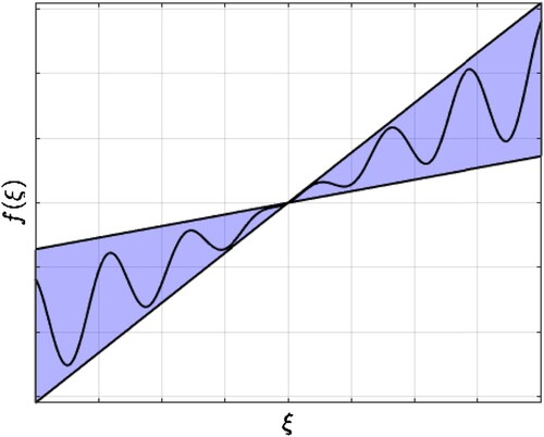The inequalities in (48(48) $\begin{array}{r}{k}_1{\xi }^2+{\alpha }_1(|\xi |)|\xi |\le \mathrm{\xi f}(\xi )\le k_2{\xi }^2-{\alpha }_2(|\xi |)|\xi |\mathrm{\forall }\xi \in \mathbb{R},\end{array}$(48) ) mean that the graph of f is ‘sandwiched’ between the straight lines $k_1\xi$ and $k_2\xi$ and is bounded away from these lines by ${\alpha }_j(|\xi |)$. A graphical illustration is shown in Figure 1.

Figure 1. Illustrative sector condition (48(48) $\begin{array}{r}{k}_1{\xi }^2+{\alpha }_1(|\xi |)|\xi |\le \mathrm{\xi f}(\xi )\le k_2{\xi }^2-{\alpha }_2(|\xi |)|\xi |\mathrm{\forall }\xi \in \mathbb{R},\end{array}$(48) ) when m = p = 1 with $0<k_1<k_2$. The straight lines have slopes $k_i$.

To link the conditions (47(47) $\begin{array}{r}⟨f(\xi )-K_1\xi ,f(\xi )-K_2\xi ⟩\le -\alpha (\Vert \xi \Vert )\Vert \xi \Vert \mathrm{\forall }\xi \in {\mathbb{R}}^p,\end{array}$(47) ) and (48(48) $\begin{array}{r}{k}_1{\xi }^2+{\alpha }_1(|\xi |)|\xi |\le \mathrm{\xi f}(\xi )\le k_2{\xi }^2-{\alpha }_2(|\xi |)|\xi |\mathrm{\forall }\xi \in \mathbb{R},\end{array}$(48) ), the following simple result on comparison functions is useful.

Lemma 5.5

If $h:(0,\mathrm{\infty })\to (0,\mathrm{\infty })$ is continuous and such that $\underset{s\to \mathrm{\infty }}{lim inf}h(s)>0$, then there exists $\alpha \in \mathcal{K}$ such that $\alpha (s)\le h(s)$ for all s>0. Furthermore, if  $\underset{s\to \mathrm{\infty }}{lim inf}h(s)=\mathrm{\infty }$, then $\alpha \in {\mathcal{K}}_{\mathrm{\infty }}$.

Although the proof of the above lemma is not difficult, it is, for completeness and for the convenience of the reader, included in the Appendix.

The corollary below provides the desired link between (47(47) $\begin{array}{r}⟨f(\xi )-K_1\xi ,f(\xi )-K_2\xi ⟩\le -\alpha (\Vert \xi \Vert )\Vert \xi \Vert \mathrm{\forall }\xi \in {\mathbb{R}}^p,\end{array}$(47) ) and (48(48) $\begin{array}{r}{k}_1{\xi }^2+{\alpha }_1(|\xi |)|\xi |\le \mathrm{\xi f}(\xi )\le k_2{\xi }^2-{\alpha }_2(|\xi |)|\xi |\mathrm{\forall }\xi \in \mathbb{R},\end{array}$(48) ).

Corollary 5.6

Let $k_1$ and $k_2$ be real scalars with $k_1<k_2$, let ${\alpha }_1,{\alpha }_2:{\mathbb{R}}_{+}\to {\mathbb{R}}_{+}$ be continuous and such that ${\alpha }_j(s)>0$ for all s>0, j = 1, 2, and (49) $\begin{array}{r}{l}_j:=\underset{s\to \mathrm{\infty }}{lim inf}{\alpha }_j(s)>0,j=1,2\end{array}$(49) If (48(48) $\begin{array}{r}{k}_1{\xi }^2+{\alpha }_1(|\xi |)|\xi |\le \mathrm{\xi f}(\xi )\le k_2{\xi }^2-{\alpha }_2(|\xi |)|\xi |\mathrm{\forall }\xi \in \mathbb{R},\end{array}$(48) ) holds, then there exists $\alpha \in \mathcal{K}$ such that $\begin{array}{r}(f(\xi )-k_1\xi )(f(\xi )-k_2\xi )\le -\alpha (|\xi |)|\xi |\mathrm{\forall }\xi \in \mathbb{R}.\end{array}$Furthermore, if $l_j=\mathrm{\infty }$ for j = 1, 2, then $\alpha \in {\mathcal{K}}_{\mathrm{\infty }}$.

Proof.

Arguments similar to those used in the proof of Sarkans and Logemann (2015, Corollary 3.13) show that if (48(48) $\begin{array}{r}{k}_1{\xi }^2+{\alpha }_1(|\xi |)|\xi |\le \mathrm{\xi f}(\xi )\le k_2{\xi }^2-{\alpha }_2(|\xi |)|\xi |\mathrm{\forall }\xi \in \mathbb{R},\end{array}$(48) ) holds, then $\begin{array}{rl}& (f(\xi )-k_1\xi )(f(\xi )-k_2\xi )\\ & \le -\frac{k_2-k_1}{2}min({\alpha }_1(|\xi |),{\alpha }_2(|\xi |))|\xi |\mathrm{\forall }\xi \in \mathbb{R}.\end{array}$The claim now follows from Lemma 5.5

Proof

Proof of Theorem 5.2

Let $S=(A,B,B_{\mathrm{e}},C,D,D_{\mathrm{e}})$ be the state-space realisation of the input-output system $(\mathbf{P},\mathbf{Q},{\mathbf{Q}}_{\mathrm{e}})$ guaranteed to exist by Theorem 4.6. As $K\in {\mathbb{S}}_{\mathrm{io}}(\mathbf{P},\mathbf{Q})$, it is clear that I−DK is invertible. Setting $L:=K(I-\mathrm{DK}{)}^{-1}$, we have that $I+\mathrm{DL}=(I-\mathrm{DK}{)}^{-1}$. Therefore, $\mathbf{P}(I+\mathrm{DL})-\mathbf{Q}L=(\mathbf{P}-\mathbf{Q}K)(I-\mathrm{DK}{)}^{-1}$, and so, $\mathbf{P}(I+\mathrm{DL})-\mathbf{Q}L$ is Hurwitz. It follows from statement (5) of Theorem 4.6 that $(A,B)$ is stabilizable. Now $(C,A)$ is observable, and a fortiori $(C,A)$ is detectable, implying that (5(5) $\begin{array}{rl}& {\mathbb{S}}_{\mathrm{ss}}(A,B,C,D)=\{K\in {\mathbb{C}}^{m\times p}:det(I-K\mathbf{G}(s))\not\equiv 0\mathrm{and}\\ & \mathbf{G}(I-K\mathbf{G}{)}^{-1}\in H^{\mathrm{\infty }}({\mathbb{C}}^{p\times m})\}.\end{array}$(5) ) holds. Furthermore, $\text{rk}(\mathbf{P}(s),\mathbf{Q}(s))=p$ for all $s\in {\overline{\mathbb{C}}}_0$ (because otherwise $\mathbf{P}-\mathbf{Q}K$ could not be Hurwitz), and thus, (43(43) $\begin{array}{rl}& {\mathbb{S}}_{\mathrm{io}}(\mathbf{P},\mathbf{Q})=\{K\in {\mathbb{C}}^{p\times m}:det(I-K\mathbf{G}(s))\not\equiv 0\text{ and}\\ & \mathbf{G}(I-K\mathbf{G}{)}^{-1}\in H^{\mathrm{\infty }}({\mathbb{C}}^{p\times m})\}.\end{array}$(43) ) is satisfied. Consequently, ${\mathbb{S}}_{\mathrm{ss}}(A,B,C,D)={\mathbb{S}}_{\mathrm{io}}(\mathbf{P},\mathbf{Q})$, whence ${\mathbb{B}}_{\mathbb{C}}(K,r)\subset {\mathbb{S}}_{\mathrm{ss}}(A,B,C,D)$ by assumption. We conclude that the hypotheses of Theorem 3.1 are satisfied.

To prove statement (1), we first note that, for all $(v,x,y)\in \mathcal{B}(S^f)$, $y=C^{K}x+D^K(f\circ y-\mathrm{Ky})+D_{\mathrm{e}}^{K}v$, where $C^K:=(I-\mathrm{DK}{)}^{-1}C$, $D^K:=(I-\mathrm{DK}{)}^{-1}D$ and $D_{\mathrm{e}}^K:=(I-\mathrm{DK}{)}^{-1}{D}_{\mathrm{e}}$, and thus, $\begin{array}{rl}& \Vert C^K\Vert \Vert x(t)\Vert +\Vert D_{\mathrm{e}}^K\Vert \Vert v(t)\Vert \ge \Vert y(t)\Vert -r\Vert D^K\Vert \Vert y(t)\Vert \\ & \text{a.e.}t\ge 0,\mathrm{\forall }(v,x,y)\in \mathcal{B}(S^f).\end{array}$By hypothesis, $r\Vert D^K\Vert <1$, and we conclude that there exists a constant b>0 such that (50) $\begin{array}{r}b(\Vert x(t)\Vert +\Vert v(t)\Vert )\ge \Vert y(t)\Vert \text{a.e.}t\ge 0,\mathrm{\forall }(v,x,y)\in \mathcal{B}(S^f).\end{array}$(50) Next we apply statement (1) of Theorem 3.1 by which there exist ${\beta }_0\in \mathcal{K}\mathcal{L}$ and ${\gamma }_0\in \mathcal{K}$ such that, for all $(v,x,y)\in \mathcal{B}(S^f)$ $\begin{array}{r}\Vert x(t)\Vert \le {\beta }_0(\Vert x(0)\Vert ,t)+{\gamma }_0(\Vert v{\Vert }_{L^{\mathrm{\infty }}(0,t)})\mathrm{\forall }t\ge 0.\end{array}$Combining this with (50(50) $\begin{array}{r}b(\Vert x(t)\Vert +\Vert v(t)\Vert )\ge \Vert y(t)\Vert \text{a.e.}t\ge 0,\mathrm{\forall }(v,x,y)\in \mathcal{B}(S^f).\end{array}$(50) ) yields, for all $(v,x,y)\in \mathcal{B}(S^f)$ (51) $\begin{array}{r}\Vert y(t)\Vert \le {\beta }_1(\Vert x(0)\Vert ,t)+\gamma (\Vert v{\Vert }_{L^{\mathrm{\infty }}(0,t)})\text{a.e.}t\ge 0,\end{array}$(51) where ${\beta }_1\in \mathcal{K}\mathcal{L}$ and $\gamma \in {\mathcal{K}}_{\mathrm{\infty }}$ are defined by ${\beta }_1(s,t):=b{\beta }_0(s,t)$ and $\gamma (s):=b({\gamma }_0(s)+s)$ for all $s,t\ge 0$. Using Proposition 5.1, there exists c>0 such that $\begin{array}{r}\Vert x(0)\Vert \le c\Vert J(f\circ y,v,y)\Vert \mathrm{\forall }(v,y)\in \mathcal{B}(\mathbf{P},\mathbf{Q},{\mathbf{Q}}_{\mathrm{e}},f),\end{array}$where x is the unique function in $W_{\mathrm{loc}}^{1,1}({\mathbb{R}}_{+},{\mathbb{R}}^n)$ such that $(v,x,y)\in \mathcal{B}(S^f)$. Hence, invoking (51(51) $\begin{array}{r}\Vert y(t)\Vert \le {\beta }_1(\Vert x(0)\Vert ,t)+\gamma (\Vert v{\Vert }_{L^{\mathrm{\infty }}(0,t)})\text{a.e.}t\ge 0,\end{array}$(51) ), we conclude that, for all $(v,y)\in \mathcal{B}(\mathbf{P},\mathbf{Q},{\mathbf{Q}}_{\mathrm{e}},f)$, $\begin{array}{r}\Vert y(t)\Vert \le \beta (\Vert J(f\circ y,v,y)\Vert ,t)+\gamma (\Vert v{\Vert }_{L^{\mathrm{\infty }}(0,t)})\text{a.e.}t\ge 0,\end{array}$where $\beta \in \mathcal{K}\mathcal{L}$ is given by $\beta (s,t):={\beta }_1(\mathrm{cs},t)$ for all $s,t\ge 0$, completing the proof of statement (1).

Statement (2) can be proved by a similar argument, with the application of statement (1) of Theorem 3.1 replaced by that of statement (2) of Theorem 3.1.

In the corollary below, we consider the situation wherein condition (44(44) $\begin{array}{r}\Vert f(\xi )-\mathrm{K\xi }\Vert \le r\Vert \xi \Vert -\alpha (\Vert \xi \Vert )\mathrm{\forall }\xi \in {\mathbb{R}}^p.\end{array}$(44) ) is only satisfied on the complement of a bounded set. It turns out that some form of stability, reminiscent of practical ISS or ISS with bias (see, for example, Jayawardhana et al., 2009, 2011; Mironchenko, 2019), is retained under this weaker assumption.

Corollary 5.7

Let $(\mathbf{P},\mathbf{Q},{\mathbf{Q}}_{\mathrm{e}})\in {\mathrm{\Sigma }}_{\mathrm{io}}$, $f:{\mathbb{R}}^p\to {\mathbb{R}}^m$ be continuous, $K\in {\mathbb{R}}^{m\times p}$ and r>0. If ${\mathbb{B}}_{\mathbb{C}}(K,r)\subset {\mathbb{S}}_{\mathrm{io}}(\mathbf{P},\mathbf{Q})$, $r\Vert D(I-\mathrm{KD}{)}^{-1}\Vert <1$, where $D:=\mathbf{G}(\mathrm{\infty })$, and there exist $\alpha \in {\mathcal{K}}_{\mathrm{\infty }}$ and a>0 such that $\begin{array}{r}\Vert f(\xi )-\mathrm{K\xi }\Vert \le r\Vert \xi \Vert -\alpha (\Vert \xi \Vert )\text{for all}\xi \in {\mathbb{R}}^p\mathrm{with}\Vert \xi \Vert \ge a,\end{array}$then there exist $\beta \in \mathcal{K}\mathcal{L}$, $\gamma \in \mathcal{K}$ and b>0 such that, for all $(v,y)\in \mathcal{B}(\mathbf{P},\mathbf{Q},{\mathbf{Q}}_{\mathrm{e}},f)$, (52) $\begin{array}{r}\Vert y(t)\Vert \le \beta (\Vert J(f\circ y,v,y)\Vert ,t)+\gamma (\Vert v{\Vert }_{L^{\mathrm{\infty }}(0,t)}+b)\text{a.e.}t\ge 0.\end{array}$(52)

Proof.

To make use of Theorem 5.2, we introduce a modified nonlinearity $\tilde{f}$ defined by $\begin{array}{r}\tilde{f}(\xi ):=\{\begin{array}{ll}f(\xi ),& \mathrm{if}\Vert \xi \Vert \ge a,\\ (\Vert \xi \Vert /a)f((a/\Vert \xi \Vert )\xi ),& \mathrm{if}0<\Vert \xi \Vert <a,\\ 0,& \mathrm{if}\xi =0.\end{array}\end{array}$Note that $\tilde{f}$ is continuous and $\begin{array}{r}\Vert \tilde{f}(\xi )-\mathrm{K\xi }\Vert \le r\Vert \xi \Vert -\tilde{\alpha }(\Vert \xi \Vert )\mathrm{\forall }\xi \in {\mathbb{R}}^p,\end{array}$where $\tilde{\alpha }\in {\mathcal{K}}_{\mathrm{\infty }}$ is given by $\begin{array}{r}\tilde{\alpha }(s):=\{\begin{array}{ll}\alpha (s),& \mathrm{if}s\ge a,\\ (s/a)\alpha (a),& \mathrm{if}0\le s<a.\end{array}\end{array}$An application of Theorem 5.2 to the system $(\mathbf{P},\mathbf{Q},{\mathbf{Q}}_{\mathrm{e}},\tilde{f})$ shows that there exist $\beta \in \mathcal{K}\mathcal{L}$ and $\gamma \in \mathcal{K}$ such that, for all $(\tilde{v},\tilde{y})\in \mathcal{B}(\mathbf{P},\mathbf{Q},{\mathbf{Q}}_{\mathrm{e}},\tilde{f})$, (53) $\begin{array}{r}\Vert \tilde{y}(t)\Vert \le \beta (\Vert J(\tilde{f}\circ \tilde{y},\tilde{v},\tilde{y})\Vert ,t)+\gamma (\Vert \tilde{v}{\Vert }_{L^{\mathrm{\infty }}(0,t)})\text{a.e.}t\ge 0.\end{array}$(53) Furthermore, if $(v,y)\in \mathcal{B}(\mathbf{P},\mathbf{Q},{\mathbf{Q}}_{\mathrm{e}},f)$, then $(v+d,y)\in \mathcal{B}(\mathbf{P},\mathbf{Q},{\mathbf{Q}}_{\mathrm{e}},\tilde{f})$, where $d(t)=f(y(t))-\tilde{f}(y(t))$ for all $t\ge 0$. Clearly, $\Vert d(t)\Vert \le \underset{\Vert \xi \Vert \le a}{max}\Vert f(\xi )-\tilde{f}(\xi )\Vert$ for all $t\ge 0$. It now follows from (53(53) $\begin{array}{r}\Vert \tilde{y}(t)\Vert \le \beta (\Vert J(\tilde{f}\circ \tilde{y},\tilde{v},\tilde{y})\Vert ,t)+\gamma (\Vert \tilde{v}{\Vert }_{L^{\mathrm{\infty }}(0,t)})\text{a.e.}t\ge 0.\end{array}$(53) ) that, for all $(v,y)\in \mathcal{B}(\mathbf{P},\mathbf{Q},{\mathbf{Q}}_{\mathrm{e}},f)$, (52(52) $\begin{array}{r}\Vert y(t)\Vert \le \beta (\Vert J(f\circ y,v,y)\Vert ,t)+\gamma (\Vert v{\Vert }_{L^{\mathrm{\infty }}(0,t)}+b)\text{a.e.}t\ge 0.\end{array}$(52) ) holds with $b:=\underset{\Vert \xi \Vert \le a}{max}\Vert \tilde{f}(\xi )-f(\xi )\Vert$.

Finally, we introduce a certain type of initial-value problem for (38(38) $\begin{array}{r}\mathbf{P}(\mathcal{D})y=\mathbf{Q}(\mathcal{D})(f\circ y)+{\mathbf{Q}}_{\mathrm{e}}(\mathcal{D})v,\end{array}$(38) ). Due to the lack of regularity of weak trajectories, it is not immediately clear how an initial-value problem for (38(38) $\begin{array}{r}\mathbf{P}(\mathcal{D})y=\mathbf{Q}(\mathcal{D})(f\circ y)+{\mathbf{Q}}_{\mathrm{e}}(\mathcal{D})v,\end{array}$(38) ) can be defined. We will now briefly explain how this can be done. To this end, we introduce the vector space $\begin{array}{r}\mathcal{J}:=\{{\mathrm{col}}_{0\le i\le \ell -1}(w^{(i)}(0)):w\in \ker \mathbf{P}(\mathcal{D})\}\subset {\mathbb{R}}^{\mathrm{\ell p}}\end{array}$and note that $\dim \mathcal{J}=\mathrm{deg}det\mathbf{P}$, as follows from statement (1) of Proposition 4.3 and statement (1) of Theorem 4.6. Moreover, $J(f\circ y,v,y)\in \mathcal{J}$ for every $(v,y)\in \mathcal{B}(\mathbf{P},\mathbf{Q},{\mathbf{Q}}_{\mathrm{e}},f)$ (because if $(v,y)\in \mathcal{B}(\mathbf{P},\mathbf{Q},{\mathbf{Q}}_{\mathrm{e}},f)$, then $(f\circ y,v,y)\in \mathcal{B}(\mathbf{P},\mathbf{Q},{\mathbf{Q}}_{\mathrm{e}})$, and thus, $y-G\star (f\circ y)-G_{\mathrm{e}}\star v\in \ker \mathbf{P}(\mathcal{D})$ by Proposition 4.3).

The next result shows that, under a suitable local invertibility conditions on the map I−Df, the assumptions of Theorem 5.2 ensure that, for every $v\in L_{\mathrm{loc}}^{\mathrm{\infty }}({\mathbb{R}}_{+},{\mathbb{R}}^{m_{\mathrm{e}}})$ and every $\zeta \in \mathcal{J}$, there exists a unique $y\in L_{\mathrm{loc}}^{\mathrm{\infty }}({\mathbb{R}}_{+},{\mathbb{R}}^p)$ such that $(v,y)\in \mathcal{B}(\mathbf{P},\mathbf{Q},{\mathbf{Q}}_{\mathrm{e}},f)$ and $J(f\circ y,v,y)=\zeta$.

Proposition 5.8

Imposing the notation and assumptions of Theorem 5.2, assume further that f is locally Lispchitz, (44(44) $\begin{array}{r}\Vert f(\xi )-\mathrm{K\xi }\Vert \le r\Vert \xi \Vert -\alpha (\Vert \xi \Vert )\mathrm{\forall }\xi \in {\mathbb{R}}^p.\end{array}$(44) ) holds with $\alpha \in \mathcal{K}$, and $f_D$ defined by (10(10) $\begin{array}{r}{f}_D(\xi ):=\mathrm{Df}(\xi )\mathrm{\forall }\xi \in {\mathbb{R}}^p\end{array}$(10) ) is of class $C^1$ with $det(I-f_D^{\prime }(\xi ))\ne 0$ for all $\xi \in {\mathbb{R}}^p$, where $D:=\mathbf{G}(\mathrm{\infty })$. Then, for all $v\in L_{\mathrm{loc}}^{\mathrm{\infty }}({\mathbb{R}}_{+},{\mathbb{R}}^{m_{\mathrm{e}}})$ and $\zeta \in \mathcal{J}$, there exists a unique $y\in L_{\mathrm{loc}}^{\mathrm{\infty }}({\mathbb{R}}_{+},{\mathbb{R}}^p)$ such that $(v,y)\in \mathcal{B}(\mathbf{P},\mathbf{Q},{\mathbf{Q}}_{\mathrm{e}},f)$ and $J(f\circ y,v,y)=\zeta$.

Trivially, the conditions involving $f_D$ are satisfied when D = 0.

Proof

Proof of Proposition 5.8

Let $S=(A,B,B_{\mathrm{e}},C,D,D_{\mathrm{e}})$ be the state-space realisation of the input-output system $(\mathbf{P},\mathbf{Q},{\mathbf{Q}}_{\mathrm{e}})$ guaranteed to exist by Theorem 4.6. As has been shown in the proof of Theorem 5.2, ${\mathbb{B}}_{\mathbb{C}}(K,r)\subset {\mathbb{S}}_{\mathrm{ss}}(A,B,C,D)$, and so, the assumptions of statement (3) of Proposition 3.2 are satisfied.

Let $v\in L_{\mathrm{loc}}^{\mathrm{\infty }}({\mathbb{R}}_{+},{\mathbb{R}}^{m_{\mathrm{e}}})$ and $\zeta \in \mathcal{J}$. Recalling the notation $y_z(t)=C{\mathrm{e}}^{\mathrm{At}}z$, $t\ge 0$ and $z\in {\mathbb{R}}^n$, and invoking Theorem 4.6, there exists $x^0\in {\mathbb{R}}^n$ such that (54) $\begin{array}{r}{\mathrm{col}}_{0\le i\le \ell -1}((y_{x^0}{)}^{(i)}(0))=\zeta ,\text{where}\ell ={\mathrm{deg}}_{\mathrm{left}}\mathbf{P}.\end{array}$(54) By statement (3) of Proposition 3.2, there exists a unique pair $(x,y)$ such that $(v,x,y)\in \mathcal{B}(S^f)$ and $x(0)=x^0$. An application of statement (1) of Proposition 5.1 shows that $(v,y)\in \mathcal{B}(\mathbf{P},\mathbf{Q},{\mathbf{Q}}_{\mathrm{e}},f)$. As $\begin{array}{r}y=\mathrm{Cx}+D(f\circ y)+D_{\mathrm{e}}v=y_{x^0}+G\star (f\circ y)+G_{\mathrm{e}}\star v,\end{array}$we have that $y-G\star (f\circ y)-G_{\mathrm{e}}\star v=y_{x^0}$, and so $J(f\circ y,v,y)=\zeta$. To show uniqueness, assume that $(v,\tilde{y})\in \mathcal{B}(\mathbf{P},\mathbf{Q},{\mathbf{Q}}_{\mathrm{e}},f)$ satisfies $J(f\circ \tilde{y},v,\tilde{y})=\zeta$. Another application of statement (1) of Proposition 5.1 shows that there exists $\tilde{x}\in W_{\mathrm{loc}}^{1,1}({\mathbb{R}}_{+},{\mathbb{R}}^n)$ such that $(v,\tilde{x},\tilde{y})\in \mathcal{B}(S^f)$ and so $\tilde{y}-G\star (f\circ \tilde{y})-G_{\mathrm{e}}\star v=y_{\tilde{x}(0)}$. Consequently, ${\mathrm{col}}_{0\le i\le \ell -1}((y_{\tilde{x}(0)}{)}^{(i)}(0))=\zeta$, and thus, appealing to (54(54) $\begin{array}{r}{\mathrm{col}}_{0\le i\le \ell -1}((y_{x^0}{)}^{(i)}(0))=\zeta ,\text{where}\ell ={\mathrm{deg}}_{\mathrm{left}}\mathbf{P}.\end{array}$(54) ), ${\mathrm{col}}_{0\le i\le \ell -1}((y_{\tilde{x}(0)}{)}^{(i)}(0))={\mathrm{col}}_{0\le i\le \ell -1}((y_{x^0}{)}^{(i)}(0))$. This in turn leads to $\begin{array}{r}{\mathrm{col}}_{0\le i\le \ell -1}(C{A}^i\tilde{x}(0))={\mathrm{col}}_{0\le i\le \ell -1}(C{A}^i{x}^0).\end{array}$It now follows from (28(28) $\begin{array}{r}\ker \left(\begin{array}{c}C\\ \mathrm{CA}\\ ⋮\\ C{A}^{\ell -1}\end{array}\right)=\{0\}.\end{array}$(28) ) that $\tilde{x}(0)=x^0$. But as $(x,y)$ is the unique pair such that $(v,x,y)\in \mathcal{B}(S^f)$ and $x(0)=x^0$, it follows that $\tilde{x}=x$ and $\tilde{y}=y$, completing the proof.

6. Examples

In this section we will illustrate the input-to-output stability results of Section 5 by three examples.

Example 6.1

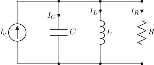
Consider the resistor-inductor-capacitor (RLC) circuit with a current source shown in Figure 2 and inspired by the electrical circuit example discussed in Jayawardhana et al. (2011, p. 34). The inductor and capacitor are modelled as linear, time-invariant components, with positive constants L (inductance) and C (capacitance). The resistor is nonlinear with current-voltage characteristic given by the (continuous) function f, that is, $I_R=f(V_R)$, where $I_R$ and $V_R$ denote the current and voltage, respectively, associated with the nonlinear resistive element. Taking into account the signs of the potential differences, an application of Kirchoff's voltage law gives that the voltages across all the components are equal, and the following differential equation $\begin{array}{r}C\frac{{\mathrm{d}}^2}{\mathrm{d}{t}^2}V+\frac{1}{L}V=-\frac{\mathrm{d}}{\mathrm{d}t}f(V)+\frac{\mathrm{d}}{\mathrm{d}t}{I}_{\mathrm{e}},\end{array}$holds, where V is the voltage and $I_{\mathrm{e}}$ is the current of the external source. Setting y = V, $u=I_R=f(y)$ and $v=I_{\mathrm{e}}$, we arrive at (55) $\begin{array}{rl}\mathbf{P}(\mathcal{D})y& =\mathbf{Q}(\mathcal{D})(f\circ y)+{\mathbf{Q}}_{\mathrm{e}}(\mathcal{D})v,\\ & \text{where}\mathbf{P}(s):=C{s}^2+\frac{1}{L},\mathbf{Q}(s):=-s,{\mathbf{Q}}_{\mathrm{e}}(s):=s,\end{array}$(55) which is of the the form (38(38) $\begin{array}{r}\mathbf{P}(\mathcal{D})y=\mathbf{Q}(\mathcal{D})(f\circ y)+{\mathbf{Q}}_{\mathrm{e}}(\mathcal{D})v,\end{array}$(38) ) with $m=m_{\mathrm{e}}=p=1$. As C and L are positive, it it is clear that, in the linear case wherein $f(y)=\mathrm{ky}$, with real gain parameter k, the associated differential equation $\begin{array}{r}C\frac{{\mathrm{d}}^2}{\mathrm{d}{t}^2}y+\frac{\mathrm{d}}{\mathrm{d}t}\mathrm{ky}+\frac{1}{L}y=0,\end{array}$is asymptotically stable if, and only if, k>0. Setting $\mathbf{G}:=\mathbf{Q}/\mathbf{P}$, we have that $\begin{array}{r}{\mathbf{G}}^k(s):=\frac{\mathbf{G}(s)}{1-k\mathbf{G}(s)}=\frac{-s}{C{s}^2+\mathrm{ks}+1/L},\end{array}$and ${\mathbf{G}}^k\in H^{\mathrm{\infty }}(\mathbb{C})$ if, and only if, k>0. As $\mathrm{rk}(\mathbf{P}(s),\mathbf{Q}(s))=1$ for all $s\in \mathbb{C}$, we conclude that $k\in {\mathbb{S}}_{\mathrm{io}}(\mathbf{P},\mathbf{Q})$ if, and only if, k>0. Using elementary calculus, it can be shown that $\begin{array}{r}\Vert {\mathbf{G}}^k{\Vert }_{H^{\mathrm{\infty }}}=|{\mathbf{G}}^k(\pm i/\sqrt{\mathrm{CL}})|=1/k\mathrm{\forall }k>0.\end{array}$Consequently, it follows from statement (1) of Theorem 5.2 and Remark 5.3 that, for every continuous function $f:\mathbb{R}\to \mathbb{R}$ satisfying (56) $\begin{array}{r}|f(\xi )-\mathrm{k\xi }|\le k|\xi |-\alpha (|\xi |)\mathrm{\forall }\xi \in \mathbb{R}\end{array}$(56) for some k>0 and $\alpha \in {\mathcal{K}}_{\mathrm{\infty }}$, there exist $\beta \in \mathcal{K}\mathcal{L}$ and $\gamma \in \mathcal{K}$ such that (45(45) $\begin{array}{r}\Vert y(t)\Vert \le \beta (\Vert J(f\circ y,v,y)\Vert ,t)+\gamma (\Vert v{\Vert }_{L^{\mathrm{\infty }}(0,t)})\text{a.e.}t\ge 0.\end{array}$(45) ) holds for all $(v,y)\in \mathcal{B}(\mathbf{P},\mathbf{Q},{\mathbf{Q}}_{\mathrm{e}},f)$, where $v=I_{\mathrm{e}}$ and y = V.

Figure 2. RLC circuit of Example 6.1.

To capture the situation when f is a so-called negative resistance element (such as a tunnel-diode see, for example, Khalil, 2002, Section 1.2.2), meaning that $f(0)=0$, $\underset{|\xi |\to 0}{lim sup}(f(\xi )/\xi )<0$, and $\mathrm{sign}(\xi )f(\xi )\to \mathrm{\infty }$ as $|\xi |\to \mathrm{\infty }$, we note that Remark 5.3 and Corollary 5.7 guarantee that, for every continuous function $f:\mathbb{R}\to \mathbb{R}$ satisfying (57) $\begin{array}{r}|f(\xi )-\mathrm{k\xi }|\le k|\xi |-\alpha (|\xi |)\text{for all}\xi \in \mathbb{R}\text{with}|\xi |\ge a\end{array}$(57) for some a, k>0 and $\alpha \in {\mathcal{K}}_{\mathrm{\infty }}$, there exist $\beta \in \mathcal{K}\mathcal{L}$, $\gamma \in \mathcal{K}$ and b>0 such that (52(52) $\begin{array}{r}\Vert y(t)\Vert \le \beta (\Vert J(f\circ y,v,y)\Vert ,t)+\gamma (\Vert v{\Vert }_{L^{\mathrm{\infty }}(0,t)}+b)\text{a.e.}t\ge 0.\end{array}$(52) ) holds for all $(v,y)\in \mathcal{B}(\mathbf{P},\mathbf{Q},{\mathbf{Q}}_{\mathrm{e}},f)$, where $v=I_{\mathrm{e}}$ and y = V.

Noting that for this example $\mathcal{J}={\mathbb{R}}^2$, it follows from Proposition 5.8 that, for every $\zeta =({\zeta }_1,{\zeta }_2{)}^T\in {\mathbb{R}}^2$, there exists a unique weak trajectory $(v,y)\in \mathcal{B}(\mathbf{P},\mathbf{Q},{\mathbf{Q}}_{\mathrm{e}},f)$) satisfying $J(f\circ y,v,y)=\zeta$. A routine calculation shows that ζ and $(y(0),\dot{y}(0){)}^T$ are related as follows $\begin{array}{r}y(0)={\zeta }_1\text{and}\dot{y}(0)={\zeta }_2+(v(0)-f(y(0))/C.\end{array}$To illustrate our results numerically, we present two simulations. The following model data are common to both: $\begin{array}{r}C=1,L=1,k=1,y(0)=\dot{y}(0)=\frac{1}{2},\end{array}$and the bounded, periodic and discontinuous forcing term $\begin{array}{r}v(t):=\{\begin{array}{ll}-a& t\in [2m,2m+1],\\ a& t\in (2m+1,2(m+1))\end{array},m\in {\mathbb{N}}_0\end{array}$where $a\ge 0$ is an amplitude parameter, with a = 0 giving rise to the unforced input-output Lur'e system. We consider two nonlinearities $f_j:\mathbb{R}\to \mathbb{R}$ given by $\begin{array}{rl}{f}_1(\xi )& :=\mathrm{sign}(\xi )g_1(|\xi |),\\ \text{with}{g}_1(\xi )& :=(k/2)min\{\mathrm{mod}(\xi ,2),1\}+(k/2)\lfloor \xi /(2k)\rfloor ,\\ \text{and}{f}_2(\xi )& :=\mathrm{k\xi }(\frac{|\xi |}{1+|\xi |}-4{\mathrm{e}}^{-|\xi |}),\end{array}$where $\lfloor x\rfloor$ denotes the largest integer less or equal to x and $\mathrm{mod}(x,z):=x-z\lfloor x/z\rfloor$, $x,z\in \mathbb{R}$, $z\ne 0$ (if x and z are integers, then $\mathrm{mod}(x,z)$ is the remainder after division of x by z). The functions $f_1$ and $f_2$ have been chosen somewhat arbitrarily to illustrate a positive- and negative-resistance element, respectively. The function $f_1$ is globally Lipschitz, but not differentiable everywhere. Graphs of the functions $f_1$ and $f_2$ are plotted in Figure 3(a,b) illustrates that $f_1$ and $f_2$, respectively, satisfy (56(56) $\begin{array}{r}|f(\xi )-\mathrm{k\xi }|\le k|\xi |-\alpha (|\xi |)\mathrm{\forall }\xi \in \mathbb{R}\end{array}$(56) ) and (57(57) $\begin{array}{r}|f(\xi )-\mathrm{k\xi }|\le k|\xi |-\alpha (|\xi |)\text{for all}\xi \in \mathbb{R}\text{with}|\xi |\ge a\end{array}$(57) ), both for some $\alpha \in {\mathcal{K}}_{\mathrm{\infty }}$. Furthermore, note that $f_2$ does not satisfy (56(56) $\begin{array}{r}|f(\xi )-\mathrm{k\xi }|\le k|\xi |-\alpha (|\xi |)\mathrm{\forall }\xi \in \mathbb{R}\end{array}$(56) ). These properties are readily verified mathematically.

Figure 3. Numerical simulation results from Example 6.1. (a) Graphs of $f_j$ (b) Graphs of $f_j(\xi )-\mathrm{k\xi }$. The dotted straight lines have slope $\pm k$. In both panels, j = 1 is shown in solid line and j = 2 in dashed-dotted line. (c) Outputs $y=y_1$ for specified values of a. (d) Outputs $y=y_2$ for specified values of a.

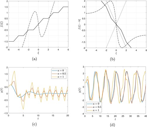
Let $(v,y_j)$ denote the unique weak trajectory of (55(55) $\begin{array}{rl}\mathbf{P}(\mathcal{D})y& =\mathbf{Q}(\mathcal{D})(f\circ y)+{\mathbf{Q}}_{\mathrm{e}}(\mathcal{D})v,\\ & \text{where}\mathbf{P}(s):=C{s}^2+\frac{1}{L},\mathbf{Q}(s):=-s,{\mathbf{Q}}_{\mathrm{e}}(s):=s,\end{array}$(55) ) with $f=f_j$, that is, $(v,y_j)\in \mathcal{B}(\mathbf{P},\mathbf{Q},{\mathbf{Q}}_{\mathrm{e}},f_j)$ for $j=1,2$. Graphs of the output trajectories plotting $y_j$ against t are shown in Figures 3(c) (j = 1) and 3(d) (j = 2). In both figures, the blue lines denote the output trajectory subject to zero forcing, which converges to zero when $f=f_1$, and is seen to boundedly oscillate when $f=f_2$. These trajectories have been plotted for comparison purposes. As expected from the estimate (45(45) $\begin{array}{r}\Vert y(t)\Vert \le \beta (\Vert J(f\circ y,v,y)\Vert ,t)+\gamma (\Vert v{\Vert }_{L^{\mathrm{\infty }}(0,t)})\text{a.e.}t\ge 0.\end{array}$(45) ), the solutions $y_1$ are bounded and we observe larger deviation from the converging solution of the unforced equation as the magnitude parameter a increases. Similar observations apply to $y_2$, but now deviations from the oscillatory unforced solution are observed–behaviour which is compatible with the practical input-to-output stability estimate (52(52) $\begin{array}{r}\Vert y(t)\Vert \le \beta (\Vert J(f\circ y,v,y)\Vert ,t)+\gamma (\Vert v{\Vert }_{L^{\mathrm{\infty }}(0,t)}+b)\text{a.e.}t\ge 0.\end{array}$(52) ) via the ‘offset’ term b.

In the next example, we provide an illustration of Corollary 5.4 (the circle criterion).

Example 6.2

The following linear input-output system is considered in Polderman and Willems (1998, Example 3.3.25) (58) $\begin{array}{rl}\mathbf{P}(\mathcal{D})y& =\mathbf{Q}(\mathcal{D})u,\text{where}\mathbf{P}(s):=(s+1{)}^2\text{and}\\ & \mathbf{Q}(s):=4s^2-3s+1.\end{array}$(58) The transfer function $\mathbf{G}(s)=\mathbf{Q}(s)/\mathbf{P}(s)=(4s^2-3s+1)/(s+1{)}^2$ is proper, but not strictly proper. Applying the feedback $u=\mathbf{Q}(\mathcal{D})(f(y)+v)$ to (58(58) $\begin{array}{rl}\mathbf{P}(\mathcal{D})y& =\mathbf{Q}(\mathcal{D})u,\text{where}\mathbf{P}(s):=(s+1{)}^2\text{and}\\ & \mathbf{Q}(s):=4s^2-3s+1.\end{array}$(58) ) leads to $\begin{array}{r}\mathbf{P}(\mathcal{D})y=\mathbf{Q}(\mathcal{D})f(y)+\mathbf{Q}(\mathcal{D})v\end{array}$which is of the form (38(38) $\begin{array}{r}\mathbf{P}(\mathcal{D})y=\mathbf{Q}(\mathcal{D})(f\circ y)+{\mathbf{Q}}_{\mathrm{e}}(\mathcal{D})v,\end{array}$(38) ) with ${\mathbf{Q}}_{\mathrm{e}}=\mathbf{Q}$. 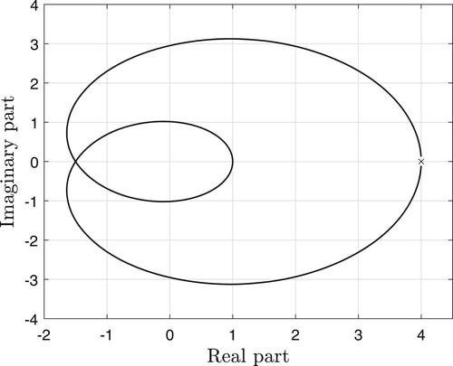To apply Corollary 5.4, we set $\mathbf{H}:=(1-k_2\mathbf{G})/(1-k_1\mathbf{G})$ for $k_1,k_2\in \mathbb{R}$, plot the Nyquist diagram of $\mathbf{G}$ in Figure 4, and consider two cases.

Figure 4. Nyquist plot for $\mathbf{G}$ in Example 6.2.

Case 1: $k_1<0=k_2$. In this case, $\mathbf{H}$ is positive real if, and only if, $1/(1-k_1\mathbf{G})$ is positive real, or, equivalently, if, and only if, (59) $\begin{array}{r}\mathrm{Re}\mathbf{G}(\mathrm{i\omega })\ge \frac{1}{k_1}\mathrm{\forall }\omega \in \mathbb{R}.\end{array}$(59) An inspection of Figure 4 yields that (59(59) $\begin{array}{r}\mathrm{Re}\mathbf{G}(\mathrm{i\omega })\ge \frac{1}{k_1}\mathrm{\forall }\omega \in \mathbb{R}.\end{array}$(59) ) holds if $k_1=k=-0.6095$. Consider a continuous nonlinearity satisfying $\begin{array}{r}k{\xi }^2+{\alpha }_1(|\xi |)|\xi |\le f(\xi )\xi \le -{\alpha }_2(|\xi |)|\xi |\mathrm{\forall }\xi \in \mathbb{R},\end{array}$for continuous functions ${\alpha }_1,{\alpha }_2:{\mathbb{R}}_{+}\to {\mathbb{R}}_{+}$, where it is assumed that ${\alpha }_1(s)>0$ and ${\alpha }_2(s)>0$ for all s>0 and (49(49) $\begin{array}{r}{l}_j:=\underset{s\to \mathrm{\infty }}{lim inf}{\alpha }_j(s)>0,j=1,2\end{array}$(49) ) holds. An application of Corollary 5.6 shows that there exists $\alpha \in \mathcal{K}$ (with $\alpha \in {\mathcal{K}}_{\mathrm{\infty }}$ if $l_j=\mathrm{\infty }$ for j = 1, 2) such that $\begin{array}{r}(f(\xi )-\mathrm{k\xi })f(\xi )\le -\alpha (|\xi |)|\xi |\mathrm{\forall }\xi \in \mathbb{R},\end{array}$which is of the form (47(47) $\begin{array}{r}⟨f(\xi )-K_1\xi ,f(\xi )-K_2\xi ⟩\le -\alpha (\Vert \xi \Vert )\Vert \xi \Vert \mathrm{\forall }\xi \in {\mathbb{R}}^p,\end{array}$(47) ) with $K_1=k$ and $K_2=0$. If $l_j=\mathrm{\infty }$ for j = 1, 2, then it follows from statement (1) of Corollary 5.4 that there exist $\beta \in \mathcal{K}\mathcal{L}$ and $\gamma \in \mathcal{K}$ such that (45(45) $\begin{array}{r}\Vert y(t)\Vert \le \beta (\Vert J(f\circ y,v,y)\Vert ,t)+\gamma (\Vert v{\Vert }_{L^{\mathrm{\infty }}(0,t)})\text{a.e.}t\ge 0.\end{array}$(45) ) holds for all $(v,y)\in \mathcal{B}(\mathbf{P},\mathbf{Q},{\mathbf{Q}}_{\mathrm{e}},f)$. Similarly, if $l_1<\mathrm{\infty }$ or $l_2<\mathrm{\infty }$ then statement (2) of Corollary 5.4 shows that there exist $\beta ,\psi \in \mathcal{K}\mathcal{L}$, $\gamma ,\varphi ,\theta \in \mathcal{K}$ and b>0 such that (45(45) $\begin{array}{r}\Vert y(t)\Vert \le \beta (\Vert J(f\circ y,v,y)\Vert ,t)+\gamma (\Vert v{\Vert }_{L^{\mathrm{\infty }}(0,t)})\text{a.e.}t\ge 0.\end{array}$(45) ) holds for all $(v,y)\in \mathcal{B}(\mathbf{P},\mathbf{Q},{\mathbf{Q}}_{\mathrm{e}},f)$ with $\Vert v{\Vert }_{L^{\mathrm{\infty }}}\le b$ and (46(46) $\begin{array}{rl}\Vert y(t)\Vert & \le \psi (\Vert J(f\circ y,v,y)\Vert ,t)+\varphi ({\int }_0^t\theta (\Vert v(\tau )\Vert )\mathrm{d}\tau )\\ & \text{a.e.}t\ge 0\end{array}$(46) ) is satisfied for every trajectory $(v,y)\in \mathcal{B}(\mathbf{P},\mathbf{Q},{\mathbf{Q}}_{\mathrm{e}},f)$.

Case 2: $k_1=0<k_2$. We note that $\mathbf{H}$ is positive real if, and only if, $1-k_2\mathbf{G}$ is positive real, or, equivalently, if, and only if, $\begin{array}{r}\mathrm{Re}\mathbf{G}(\mathrm{i\omega })\le \frac{1}{k_2}\mathrm{\forall }\omega \in \mathbb{R}.\end{array}$It follows from Figure 4 that the above condition is satisfied for $k_2=1/4$. Consider a continuous nonlinearity satisfying $\begin{array}{r}{\alpha }_1(|\xi |)|\xi |\le f(\xi )\xi \le {\xi }^2/4-{\alpha }_2(|\xi |)|\xi |\mathrm{\forall }\xi \in \mathbb{R},\end{array}$where ${\alpha }_1,{\alpha }_2:{\mathbb{R}}_{+}\to {\mathbb{R}}_{+}$ are continuous, ${\alpha }_1(s)>0$ and ${\alpha }_2(s)>0$ for all s>0 and (49(49) $\begin{array}{r}{l}_j:=\underset{s\to \mathrm{\infty }}{lim inf}{\alpha }_j(s)>0,j=1,2\end{array}$(49) ) holds. Corollaries 5.4 and 5.6 allow us to derive conclusions similar to those in Case 1. We leave the details to the reader.

In the third and final example, we study a simple multivariable system.

Example 6.3

Consider the input-output Lur'e system (60) $\begin{array}{r}\mathbf{P}(\mathcal{D})y=\mathbf{Q}(\mathcal{D})f(y)+{\mathbf{Q}}_{\mathrm{e}}(\mathcal{D})v,\end{array}$(60) where $\begin{array}{rl}\mathbf{P}(s)& :=\left(\begin{array}{cc}s& 0\\ s(s+1)& s\end{array}\right)=s\left(\begin{array}{cc}1& 0\\ s+1& 1\end{array}\right),\\ \mathbf{Q}(s)& :=\left(\begin{array}{cc}s+1& 0\\ s^2& 1\end{array}\right),{\mathbf{Q}}_{\mathrm{e}}:=\mathbf{Q},\end{array}$and $f:{\mathbb{R}}^2\to {\mathbb{R}}^2$ is continuous. As usual, we set $\mathbf{G}:={\mathbf{P}}^{-1}\mathbf{Q}$ and thus, $\begin{array}{r}\mathbf{G}(s)=\frac{1}{s}\left(\begin{array}{cc}s+1& 0\\ -(2s+1)& 1\end{array}\right).\end{array}$Furthermore, defining $\begin{array}{r}L:=\left(\begin{array}{cc}1& 0\\ 1& 1\end{array}\right),\end{array}$it is a routine exercise to show that $I+\mathrm{\lambda L}\mathbf{G}$ is positive real if, and only if, $\lambda \in [0,2{\lambda }^{\ast }]$, where ${\lambda }^{\ast }:=1+\sqrt{2}$. It follows from Logemann and Townley (1997, Lemma 3.10) that (61) $\begin{array}{r}\Vert L\mathbf{G}(I+\mathrm{\lambda L}\mathbf{G}{)}^{-1}{\Vert }_{H^{\mathrm{\infty }}}=\frac{1}{\lambda }\mathrm{\forall }\lambda \in (0,{\lambda }^{\ast }].\end{array}$(61) Consequently, $\begin{array}{r}\Vert \mathbf{G}(I+\mathrm{\lambda L}\mathbf{G}{)}^{-1}{\Vert }_{H^{\mathrm{\infty }}}\le \frac{\Vert L^{-1}\Vert }{\lambda }\mathrm{\forall }\lambda \in (0,{\lambda }^{\ast }],\end{array}$and, as $(\mathbf{G}(I+\mathrm{\lambda L}\mathbf{G}{)}^{-1})(0)=(\mathrm{\lambda L}{)}^{-1}$, the above equation yields that $\begin{array}{r}\Vert \mathbf{G}(I+\mathrm{\lambda L}\mathbf{G}{)}^{-1}{\Vert }_{H^{\mathrm{\infty }}}=\frac{\Vert L^{-1}\Vert }{\lambda }=\frac{\sqrt{3+\sqrt{5}}}{\lambda \sqrt{2}}\mathrm{\forall }\lambda \in (0,{\lambda }^{\ast }].\end{array}$As $\mathrm{rk}(\mathbf{P}(s),\mathbf{Q}(s))=2$ for all $s\in \mathbb{C}$, we conclude that $-\mathrm{\lambda L}\in {\mathbb{S}}_{\mathrm{io}}(\mathbf{P},\mathbf{Q})$ for all $\lambda \in (0,{\lambda }^{\ast }]$. An application of statement (1) of Theorem 5.2 and Remark 5.3 with $K:=-\mathrm{\lambda L}$, $\lambda \in (0,{\lambda }^{\ast }]$, shows that, for every continuous function $f:{\mathbb{R}}^2\to {\mathbb{R}}^2$ for which there exist $\lambda \in (0,{\lambda }^{\ast }]$ and $\alpha \in {\mathcal{K}}_{\mathrm{\infty }}$ such that $\begin{array}{rl}\Vert f(\xi )+\mathrm{\lambda L\xi }\Vert & \le \frac{\lambda }{\Vert L^{-1}\Vert }\Vert \xi \Vert -\alpha (\Vert \xi \Vert )\\ & =\frac{\lambda \sqrt{2}}{\sqrt{3+\sqrt{5}}}\Vert \xi \Vert -\alpha (\Vert \xi \Vert )\mathrm{\forall }\xi \in {\mathbb{R}}^2,\end{array}$there exist $\beta \in \mathcal{K}\mathcal{L}$ and $\gamma \in \mathcal{K}$ such that (45(45) $\begin{array}{r}\Vert y(t)\Vert \le \beta (\Vert J(f\circ y,v,y)\Vert ,t)+\gamma (\Vert v{\Vert }_{L^{\mathrm{\infty }}(0,t)})\text{a.e.}t\ge 0.\end{array}$(45) ) holds for all $(v,y)\in \mathcal{B}(\mathbf{P},\mathbf{Q},{\mathbf{Q}}_{\mathrm{e}},f)$.

Now consider system (60(60) $\begin{array}{r}\mathbf{P}(\mathcal{D})y=\mathbf{Q}(\mathcal{D})f(y)+{\mathbf{Q}}_{\mathrm{e}}(\mathcal{D})v,\end{array}$(60) ) with $\mathbf{P}(s)$ replaced by $\tilde{\mathbf{P}}(s):=\mathbf{P}(s)L^{-1}$, that is, $\begin{array}{r}\tilde{\mathbf{P}}(\mathcal{D})y=\mathbf{Q}(\mathcal{D})f(y)+{\mathbf{Q}}_{\mathrm{e}}(\mathcal{D})v,\end{array}$where $\begin{array}{r}\tilde{\mathbf{P}}(s):=\left(\begin{array}{cc}s& 0\\ s^2& s\end{array}\right)=s\left(\begin{array}{cc}1& 0\\ s& 1\end{array}\right)\end{array}$and the polynomial matrices $\mathbf{Q}$ and ${\mathbf{Q}}_{\mathrm{e}}$ are as before. We set $\tilde{\mathbf{G}}:={\tilde{\mathbf{P}}}^{-1}\mathbf{Q}=L\mathbf{G}$, and so, $\begin{array}{r}\tilde{\mathbf{G}}(s)=\frac{1}{s}\left(\begin{array}{cc}s+1& 0\\ -s& 1\end{array}\right).\end{array}$Setting ${\tilde{\mathbf{G}}}^k:=\tilde{\mathbf{G}}(I-k\tilde{\mathbf{G}}{)}^{-1}$, it follows from (61(61) $\begin{array}{r}\Vert L\mathbf{G}(I+\mathrm{\lambda L}\mathbf{G}{)}^{-1}{\Vert }_{H^{\mathrm{\infty }}}=\frac{1}{\lambda }\mathrm{\forall }\lambda \in (0,{\lambda }^{\ast }].\end{array}$(61) ) that $\begin{array}{r}\Vert {\tilde{\mathbf{G}}}^k{\Vert }_{H^{\mathrm{\infty }}}=\frac{1}{|k|}\mathrm{\forall }k\in [-{\lambda }^{\ast },0)\end{array}$Obviously, $\mathrm{rk}(\tilde{\mathbf{P}}(s),\mathbf{Q}(s))=2$ for all $s\in \mathbb{C}$, and thus, $\mathrm{kI}\in {\mathbb{S}}_{\mathrm{io}}(\mathbf{P},\mathbf{Q})$ for all $k\in [-{\lambda }^{\ast },0)$. An application of statement (2) of Theorem 5.2 and Remark 5.3 with K: = kI, $k\in [-{\lambda }^{\ast },0)$, shows that, for every continuous function $f:{\mathbb{R}}^2\to {\mathbb{R}}^2$ for which there exist $k\in [-{\lambda }^{\ast },0)$ and $\alpha \in \mathcal{K}$ such that (62) $\begin{array}{r}\Vert f(\xi )-\mathrm{k\xi }\Vert \le |k|\Vert \xi \Vert -\alpha (\Vert \xi \Vert )\mathrm{\forall }\xi \in {\mathbb{R}}^2,\end{array}$(62) there exist $\beta ,\psi \in \mathcal{K}\mathcal{L}$, $\gamma ,\varphi ,\theta \in \mathcal{K}$ and b>0 such that (45(45) $\begin{array}{r}\Vert y(t)\Vert \le \beta (\Vert J(f\circ y,v,y)\Vert ,t)+\gamma (\Vert v{\Vert }_{L^{\mathrm{\infty }}(0,t)})\text{a.e.}t\ge 0.\end{array}$(45) ) holds for all $(v,y)\in \mathcal{B}(\tilde{\mathbf{P}},\mathbf{Q},{\mathbf{Q}}_{\mathrm{e}},f)$ with $\Vert b{\Vert }_{L^{\mathrm{\infty }}}\le b$ and (46(46) $\begin{array}{rl}\Vert y(t)\Vert & \le \psi (\Vert J(f\circ y,v,y)\Vert ,t)+\varphi ({\int }_0^t\theta (\Vert v(\tau )\Vert )\mathrm{d}\tau )\\ & \text{a.e.}t\ge 0\end{array}$(46) ) is satisfied for all $(v,y)\in \mathcal{B}(\tilde{\mathbf{P}},\mathbf{Q},{\mathbf{Q}}_{\mathrm{e}},f)$.

Finally, let us analyse the special case wherein $k=-{\lambda }^{\ast }$ and f is a saturation nonlinearity of the form $\begin{array}{r}{f}_a(\xi ):=\{\begin{array}{ll}-\xi ,& \mathrm{if}\Vert \xi \Vert \le a,\\ -(a/\Vert \xi \Vert )\xi ,& \mathrm{if}\Vert \xi \Vert >a,\end{array}\text{where}a>0.\end{array}$Then (63) $\begin{array}{rl}\Vert f_a(\xi )-\mathrm{k\xi }\Vert & =\Vert f_a(\xi )+{\lambda }^{\ast }\xi \Vert \\ & =\{\begin{array}{ll}\sqrt{2}\Vert \xi \Vert ,& \mathrm{if}\Vert \xi \Vert \le a,\\ (1+\sqrt{2})\Vert \xi \Vert -a,& \mathrm{if}\Vert \xi \Vert >a,\end{array}\end{array}$(63) whence $\begin{array}{rl}\Vert f_a(\xi )-\mathrm{k\xi }\Vert & \le (1+\sqrt{2})\Vert \xi \Vert -{\alpha }_a(\Vert \xi \Vert )=|k|\Vert \xi \Vert -{\alpha }_a(\Vert \xi \Vert )\\ & \mathrm{\forall }\xi \in {\mathbb{R}}^2,\end{array}$where ${\alpha }_a\in \mathcal{K}$ is given by $\begin{array}{r}{\alpha }_a(s):=\{\begin{array}{ll}s/2,& \mathrm{if}0\le s\le a,\\ \mathrm{as}/(s+a),& \mathrm{if}s>a.\end{array}\end{array}$Hence (62(62) $\begin{array}{r}\Vert f(\xi )-\mathrm{k\xi }\Vert \le |k|\Vert \xi \Vert -\alpha (\Vert \xi \Vert )\mathrm{\forall }\xi \in {\mathbb{R}}^2,\end{array}$(62) ) holds with $f=f_a$, and thus, for every a>0, there exist comparison functions $\beta ,\psi \in \mathcal{K}\mathcal{L}$, $\gamma ,\varphi ,\theta \in \mathcal{K}$ and a constant b>0 such that (45(45) $\begin{array}{r}\Vert y(t)\Vert \le \beta (\Vert J(f\circ y,v,y)\Vert ,t)+\gamma (\Vert v{\Vert }_{L^{\mathrm{\infty }}(0,t)})\text{a.e.}t\ge 0.\end{array}$(45) ) holds for all $(v,y)\in \mathcal{B}(\tilde{\mathbf{P}},\mathbf{Q},{\mathbf{Q}}_{\mathrm{e}},f_a)$ with $\Vert b{\Vert }_{L^{\mathrm{\infty }}}\le b$ and (46(46) $\begin{array}{rl}\Vert y(t)\Vert & \le \psi (\Vert J(f\circ y,v,y)\Vert ,t)+\varphi ({\int }_0^t\theta (\Vert v(\tau )\Vert )\mathrm{d}\tau )\\ & \text{a.e.}t\ge 0\end{array}$(46) ) is satisfied for all $(v,y)\in \mathcal{B}(\tilde{\mathbf{P}},\mathbf{Q},{\mathbf{Q}}_{\mathrm{e}},f_a)$. Finally, (63(63) $\begin{array}{rl}\Vert f_a(\xi )-\mathrm{k\xi }\Vert & =\Vert f_a(\xi )+{\lambda }^{\ast }\xi \Vert \\ & =\{\begin{array}{ll}\sqrt{2}\Vert \xi \Vert ,& \mathrm{if}\Vert \xi \Vert \le a,\\ (1+\sqrt{2})\Vert \xi \Vert -a,& \mathrm{if}\Vert \xi \Vert >a,\end{array}\end{array}$(63) ) necessitates that any $\alpha \in \mathcal{K}$ for which (62(62) $\begin{array}{r}\Vert f(\xi )-\mathrm{k\xi }\Vert \le |k|\Vert \xi \Vert -\alpha (\Vert \xi \Vert )\mathrm{\forall }\xi \in {\mathbb{R}}^2,\end{array}$(62) ) holds with $f=f_a$ and $k=-{\lambda }^{\ast }$ satisfies $\alpha (\Vert \xi \Vert )\le a$ for all $\xi \in {\mathbb{R}}^2$, that is, α is bounded. Consequently, (62(62) $\begin{array}{r}\Vert f(\xi )-\mathrm{k\xi }\Vert \le |k|\Vert \xi \Vert -\alpha (\Vert \xi \Vert )\mathrm{\forall }\xi \in {\mathbb{R}}^2,\end{array}$(62) ) cannot hold with $\alpha \in {\mathcal{K}}_{\mathrm{\infty }}$, and therefore, we should not expect the conclusions of statement (1) of Theorem 5.2 to hold in the current scenario.

7. Conclusions

We have studied a class of forced continuous-time Lur'e systems obtained by applying nonlinear feedback to a higher-order linear differential equation which defines an input-output system in the sense of behavioural systems theory. A stability theory has been developed for this class of systems with the underlying stability concepts being input-output versions of the input-to-state stability and strong integral input-to-state properties for nonlinear state-space control systems. Our main results are Theorem 5.2 and Corollary 5.4. Theorem 5.2 is reminiscent of the complexified Aizerman conjecture, and states that if all complex gains in a certain ball are stabilising for the associated unforced, linear input-output system, then stability for the corresponding input-output Lur'e system is ensured for all nonlinearities satisfying the corresponding ‘nonlinear’ ball condition (44(44) $\begin{array}{r}\Vert f(\xi )-\mathrm{K\xi }\Vert \le r\Vert \xi \Vert -\alpha (\Vert \xi \Vert )\mathrm{\forall }\xi \in {\mathbb{R}}^p.\end{array}$(44) ). Corollary 5.4 is a novel version of the circle criterion, the hypotheses of which can be checked graphically in the single-input single-output case, although the result is valid in the general multivariable case.

The ISS theory for controlled state-space Lur'e systems developed in Sarkans and Logemann (2015) and Guiver and Logemann (2020) provide key tools for the proof of our main results. For this suitable state-state space realisations are required (or, more accurately, relationships between the behaviours of state-space and input-output Lur'e systems) which can be found in Theorem 4.6 and Proposition 5.1, and are of some independent interest. Whilst these results do show that stability of higher-order input-output Lur'e systems can be resolved by converting to a state-space formulation, in practice this is often unsatisfactory. Indeed, many control systems are naturally specified in input-output form and state-space realisations frequently introduce ‘unphysical’ variables irrelevant to the problem under consideration. The availability of stability criteria formulated in terms of the input-output model, such as Theorem 5.2 and Corollary 5.4, is therefore of key importance.

By way of potential future work, it has recently been commented in Sepulchre et al. (2022) that, roughly, incremental stability concepts are more important than stability notions alone. In fact, the work (Sepulchre et al., 2022) notes that incremental stability used to have more prominence in the control theory community than perhaps it currently does, and that attention should refocus on this area. Incremental stability broadly refers to bounding the difference of two arbitrary trajectories of a given system; see, for instance Aminzare and Sontagy (2014), Angeli (2002), and Rüffer et al. (2013). The recent works (Gilmore et al., 2020, 2021; Guiver et al., 2019) have shown how many absolute stability criteria generalise to ensure incremental stability for various forced state-space Lur'e systems, and we expect that input-output versions of some of these results could be derived.

Statements and declarations

The Matlab routines used to generate the figures in Section 6 are available from the corresponding author on request. Data sharing is not otherwise applicable to this article as no other datasets were generated or analysed during the current study.

Disclosure statement

The authors have no relevant financial or non-financial interests to disclose.

Additional information

Funding

Chris Guiver's contribution to this work was supported by a Personal Research Fellowship from the Royal Society of Edinburgh (RSE) [REF2168].

Appendix

Here we provide proofs of Proposition 2.2, and Lemmas 2.3 and 5.5.

Proof

Proof of Proposition 2.2

To prove statement (1), denote the entries of $\mathbf{P}$, $\mathbf{Q}$ and $\mathbf{G}={\mathbf{P}}^{-1}\mathbf{Q}$ by ${\mathbf{P}}_{\mathrm{ij}}$, ${\mathbf{Q}}_{\mathrm{ij}}$ and ${\mathbf{G}}_{\mathrm{ij}}$, respectively. Choose $i\in \{1,\dots ,p\}$ and $j\in \{1,\dots ,m\}$ such that $\mathrm{deg}{\mathbf{Q}}_{\mathrm{ij}}=\mathrm{deg}\mathbf{Q}$. As ${\mathbf{Q}}_{\mathrm{ij}}=\sum _{l=1}^p{\mathbf{P}}_{\mathrm{il}}{\mathbf{G}}_{\mathrm{lj}}$, we conclude that (A1) $\begin{array}{r}\mathrm{deg}\mathbf{Q}=\mathrm{deg}{\mathbf{Q}}_{\mathrm{ij}}\le \underset{1\le l\le p}{max}(\mathrm{deg}{\mathbf{P}}_{\mathrm{il}}-{\mathrm{deg}}_{\mathrm{rel}}{\mathbf{G}}_{\mathrm{lj}}).\end{array}$(A1) Let $l_0\in \{1,\dots ,p\}$ be such that the maximum on the RHS of (A1(A1) $\begin{array}{r}\mathrm{deg}\mathbf{Q}=\mathrm{deg}{\mathbf{Q}}_{\mathrm{ij}}\le \underset{1\le l\le p}{max}(\mathrm{deg}{\mathbf{P}}_{\mathrm{il}}-{\mathrm{deg}}_{\mathrm{rel}}{\mathbf{G}}_{\mathrm{lj}}).\end{array}$(A1) ) is achieved for $l=l_0$. It follows from (A1(A1) $\begin{array}{r}\mathrm{deg}\mathbf{Q}=\mathrm{deg}{\mathbf{Q}}_{\mathrm{ij}}\le \underset{1\le l\le p}{max}(\mathrm{deg}{\mathbf{P}}_{\mathrm{il}}-{\mathrm{deg}}_{\mathrm{rel}}{\mathbf{G}}_{\mathrm{lj}}).\end{array}$(A1) ) that $\begin{array}{rl}{\mathrm{deg}}_{\mathrm{rel}}({\mathbf{P}}^{-1}\mathbf{Q})& ={\mathrm{deg}}_{\mathrm{rel}}\mathbf{G}\le {\mathrm{deg}}_{\mathrm{rel}}{\mathbf{G}}_{l_{0}j}\le \mathrm{deg}{\mathbf{P}}_{i{l}_0}-\mathrm{deg}\mathbf{Q}\\ & \le \mathrm{deg}\mathbf{P}-\mathrm{deg}\mathbf{Q}.\end{array}$We proceed to establish statement (2). Let $\mathbf{L},\mathbf{U}\in \mathbb{R}[s{]}^{p\times p}$ be such that $det\mathbf{L}(s)\not\equiv 0$, $\mathbf{U}$ is unimodular and $\mathbf{U}\mathbf{P}$ is row reduced. It is sufficient to show that $\mathrm{deg}(\mathbf{L}\mathbf{P})\ge \mathrm{deg}(\mathbf{U}\mathbf{P})$. Let ${\rho }_1,\dots ,{\rho }_p$ be the row degrees of $\mathbf{U}\mathbf{P}$ and set $\begin{array}{r}\mathbf{D}(s):={\mathrm{diag}}_{1\le j\le p}(s^{{\rho }_j}).\end{array}$Using statement (2) of Lemma 2.1, we conclude that the limit matrix $\begin{array}{r}R:=\underset{|s|\to \mathrm{\infty }}{lim}{\mathbf{D}}^{-1}(s)\mathbf{U}(s)\mathbf{P}(s)\in {\mathbb{R}}^{p\times p}\end{array}$is invertible. Therefore, as $\mathbf{L}\mathbf{P}=(\mathbf{L}{\mathbf{U}}^{-1}\mathbf{D})({\mathbf{D}}^{-1}\mathbf{U}\mathbf{P})$, we may conclude that (A2) $\begin{array}{r}\mathrm{deg}(\mathbf{L}\mathbf{P})=\mathrm{deg}(\mathbf{L}{\mathbf{U}}^{-1}\mathbf{D}).\end{array}$(A2) Furthermore, writing $\begin{array}{r}\mathbf{L}{\mathbf{U}}^{-1}=({\mathbf{v}}_1,\dots ,{\mathbf{v}}_p),\text{where}{\mathbf{v}}_j\in \mathbb{R}[s{]}^p,j=1,\dots ,p,\end{array}$we have that $\begin{array}{r}\mathbf{L}(s){\mathbf{U}}^{-1}(s)\mathbf{D}(s)=(s^{{\rho }_1}{\mathbf{v}}_1(s),\dots ,s^{{\rho }_p}{\mathbf{v}}_p(s))\end{array}$As $det(\mathbf{L}(s){\mathbf{U}}^{-1}(s))\not\equiv 0$, we see that ${\mathbf{v}}_j(s)\not\equiv 0$, $j=1,\dots ,p$, and thus $\begin{array}{r}\mathrm{deg}(s^{{\rho }_j}{\mathbf{v}}_j(s))\ge {\rho }_j,j=1,\dots ,p,\end{array}$implying that $\begin{array}{r}\mathrm{deg}(\mathbf{L}{\mathbf{U}}^{-1}\mathbf{D})=\underset{1\le j\le p}{max}\mathrm{deg}(s^{{\rho }_j}{\mathbf{v}}_j(s))\ge \underset{1\le j\le p}{max}{\rho }_j=\mathrm{deg}(\mathbf{U}\mathbf{P}).\end{array}$Hence, by (A2(A2) $\begin{array}{r}\mathrm{deg}(\mathbf{L}\mathbf{P})=\mathrm{deg}(\mathbf{L}{\mathbf{U}}^{-1}\mathbf{D}).\end{array}$(A2) ), $\mathrm{deg}(\mathbf{L}\mathbf{P})\ge \mathrm{deg}(\mathbf{U}\mathbf{P})$, showing that $\mathrm{deg}(\mathbf{U}\mathbf{P})={\mathrm{deg}}_{\mathrm{left}}\mathbf{P}$.

Statement (3) follows from statement (2) and the fact that there exists a unimodular matrix $\mathbf{U}\in \mathbb{R}[s{]}^{p\times p}$ such that $\mathbf{U}\mathbf{P}$ is row reduced (see statement (1) of Lemma 2.1).

To prove statements (4) and (5), we use statement (1) of Lemma 2.1 which guarantees the existence of unimodular $\mathbf{U}\in \mathbb{R}[s{]}^{p\times p}$ such that $\mathbf{U}\mathbf{P}$ is row reduced. By statement (2), ${\mathrm{deg}}_{\mathrm{left}}\mathbf{P}=\mathrm{deg}(\mathbf{U}\mathbf{P})$ and thus, $\begin{array}{rl}{\mathrm{deg}}_{\mathrm{left}}\mathbf{P}& =\mathrm{deg}(\mathbf{U}\mathbf{P})=\underset{1\le j\le p}{max}{r}_j(\mathbf{U}\mathbf{P})\le \sum _{j=1}^p{r}_j(\mathbf{U}\mathbf{P})=\mathrm{deg}det(\mathbf{U}\mathbf{P})\\ & =\mathrm{deg}det\mathbf{P},\end{array}$showing that statement (4) holds. Moreover, since $\mathbf{G}=(\mathbf{U}\mathbf{P}{)}^{-1}(\mathbf{U}\mathbf{Q})$, statement (1) yields that (A3) $\begin{array}{r}{\mathrm{deg}}_{\mathrm{rel}}\mathbf{G}\le \mathrm{deg}(\mathbf{U}\mathbf{P})-\mathrm{deg}(\mathbf{U}\mathbf{Q})={\mathrm{deg}}_{\mathrm{left}}\mathbf{P}-\mathrm{deg}(\mathbf{U}\mathbf{Q}).\end{array}$(A3) By hypothesis, $\mathbf{Q}(s)\not\equiv 0$, and so, $\mathbf{U}(s)\mathbf{Q}(s)\not\equiv 0$, whence $\mathrm{deg}(\mathbf{U}\mathbf{Q})\ge 0$. Invoking (A3(A3) $\begin{array}{r}{\mathrm{deg}}_{\mathrm{rel}}\mathbf{G}\le \mathrm{deg}(\mathbf{U}\mathbf{P})-\mathrm{deg}(\mathbf{U}\mathbf{Q})={\mathrm{deg}}_{\mathrm{left}}\mathbf{P}-\mathrm{deg}(\mathbf{U}\mathbf{Q}).\end{array}$(A3) ) shows that ${\mathrm{deg}}_{\mathrm{left}}\mathbf{P}\ge {\mathrm{deg}}_{\mathrm{rel}}\mathbf{G}$, establishing statement (5).

Finally, we proceed to prove statement (6). By statement (3) there exists unimodular $\mathbf{U}\in \mathbb{R}[s{]}^{p\times p}$ such that $\mathrm{deg}(\mathbf{U}\mathbf{P})=0$. This means that there exists $\mathrm{\Gamma }\in {\mathbb{R}}^{p\times p}$ such that $\mathbf{U}(s)\mathbf{P}(s)\equiv \mathrm{\Gamma }$. As $det(\mathbf{U}(s)\mathbf{P}(s))\not\equiv 0$, we conclude that Γ is invertible. Thus, ${\mathbf{P}}^{-1}={\mathrm{\Gamma }}^{-1}\mathbf{U}\in \mathbb{R}[s{]}^{p\times p}$, showing that $\mathbf{P}$ is unimodular.

Proof

Proof of Lemma 2.3

Let $u\in W_{\mathrm{loc}}^{l,q}({\mathbb{R}}_{+},{\mathbb{R}}^m)$. We may assume that $l+d\ge 1$. By a well-known result on the differentiation of a convolution (see, for instance, Doetsch, 1950, Kapitel 2, Section 14, Satz 10), (A4) $\begin{array}{r}(G\star u{)}^{\prime }=G_0^{\prime }\star u+G_0(0)u+\mathbf{G}(\mathrm{\infty })u^{\prime }.\end{array}$(A4)

We note that if $d\ge 1$, then $\mathbf{G}(\mathrm{\infty })=0$ and $G_0=G$. By differentiating (A4(A4) $\begin{array}{r}(G\star u{)}^{\prime }=G_0^{\prime }\star u+G_0(0)u+\mathbf{G}(\mathrm{\infty })u^{\prime }.\end{array}$(A4) ) repeatedly, we conclude that $G\star u\in W_{\mathrm{loc}}^{l,q}({\mathbb{R}}_{+},{\mathbb{R}}^p)$. If d = 1, then (A4(A4) $\begin{array}{r}(G\star u{)}^{\prime }=G_0^{\prime }\star u+G_0(0)u+\mathbf{G}(\mathrm{\infty })u^{\prime }.\end{array}$(A4) ) implies that $G\star u\in W_{\mathrm{loc}}^{l+1,q}({\mathbb{R}}_{+},{\mathbb{R}}^p)$. Moreover, if $d\ge 2$, then the initial-value theorem (see, for example, Doetsch, 1950, Kapitel 14, Section 2, Satz 4 or Zemanian, 1987, Corollary 8.6-1a) guarantees that $\begin{array}{r}{G}_0(0)=G_0^{\prime }(0)=\dots =G_0^{(d-2)}(0)=0,\end{array}$and repeated differentiation of (A4(A4) $\begin{array}{r}(G\star u{)}^{\prime }=G_0^{\prime }\star u+G_0(0)u+\mathbf{G}(\mathrm{\infty })u^{\prime }.\end{array}$(A4) ) shows that $G\star u\in W_{\mathrm{loc}}^{l+d,q}({\mathbb{R}}_{+},{\mathbb{R}}^p)$. Finally, in each case, the process of repeated differentiation leads to (3(3) $\begin{array}{r}(G\star u{)}^{(l+d)}=\{\begin{array}{ll}\begin{array}{l}{\displaystyle G_0^{(l)}\star u+\mathbf{G}(\mathrm{\infty })u^{(l)}}\\ {\displaystyle +\sum _{i=0}^{l-1}{G}_0^{(l-1-i)}(0)u^{(i)},}\end{array}& \mathrm{if}d=0,\\ \begin{array}{l}{\displaystyle G^{(l+d)}\star u}\\ +\sum _{i=0}^l{G}^{(l+d-1-i)}(0)u^{(i)},\end{array}& \mathrm{if}d\ge 1.\end{array}\end{array}$(3) ).

Proof

Proof of Lemma 5.5

Define $\beta :{\mathbb{R}}_{+}\to {\mathbb{R}}_{+}$ by $\beta (0):=0$ and $\begin{array}{r}\beta (s):=\underset{t\in [s,\mathrm{\infty })}{inf}min(h(t),t)\mathrm{\forall }s>0.\end{array}$The function β is continuous and non-decreasing, $\beta (s)>0$ and $\beta (s)\le h(s)$ for all s>0. Furthermore, if $\underset{s\to \mathrm{\infty }}{lim inf}h(s)=\mathrm{\infty }$, then $\beta (s)\to \mathrm{\infty }$ as $s\to \mathrm{\infty }$. Setting $\begin{array}{r}\alpha (s):=\frac{s}{s+1}\beta (s)\mathrm{\forall }s\ge 0,\end{array}$we have that $\alpha \in \mathcal{K}$, $\alpha (s)<\beta (s)\le h(s)$ for all s>0, and, if $\underset{s\to \mathrm{\infty }}{lim inf}h(s)=\mathrm{\infty }$, then $\alpha \in {\mathcal{K}}_{\mathrm{\infty }}$.

References

- Ambrosetti, A., & Prodi, G. (1993). A primer of nonlinear analysis, Cambridge Studies in Advanced Mathematics, vol. 34, Cambridge University Press.
- Aminzare, Z., & Sontagy, E. D. (2014). Contraction methods for nonlinear systems: A brief introduction and some open problems. In 53rd IEEE conference on decision and control (pp. 3835–3847). IEEE.
- Angeli, D. (2002). A Lyapunov approach to the incremental stability properties. IEEE Transactions on Automatic Control, 47(3), 410–421. https://doi.org/10.1109/9.989067
- Arcak, M., & Teel, A. (2002). Input-to-state stability for a class of Lurie systems. Automatica Journal of IFAC, 38(11), 1945–1949. https://doi.org/10.1016/S0005-1098(02)00100-0
- Blomberg, H., & Ylinen, R. (1983). Algebraic theory for multivariable linear systems, Mathematics in Science and Engineering, vol. 166, Academic Press Inc.
- Boiko, I. M., Kuznetsov, N. V., Mokaev, R. N., Mokaev, T. N., Yuldashev, M. V., & Yuldashev, R. V. (2022). On counter-examples to Aizerman and Kalman conjectures. International Journal of Control, 95(4), 906–913. https://doi.org/10.1080/00207179.2020.1830304
- Brockett, R. W., & Willems, J. L. (1965a). Frequency domain stability criteria. I. IEEE Transactions on Automatic Control, AC-10(3), 255–261. https://doi.org/10.1109/TAC.1965.1098143
- Brockett, R. W., & Willems, J. L. (1965b). Frequency domain stability criteria. II. IEEE Trans. Automatic Control, AC-10(4), 407–413. https://doi.org/10.1109/TAC.1965.1098198
- Carrasco, J., & Heath, W. P. (2021). Absolute stability. In J. Webster (Ed.), Wiley encyclopedia of electrical and electronics engineering (pp. 1–12). John Wiley & Sons, Ltd.
- Carrasco, J., Turner, M. C., & Heath, W. P. (2016). Zames-Falb multipliers for absolute stability: from O'Shea's contribution to convex searches. European Journal of Control, 28, 1–19. https://doi.org/10.1016/j.ejcon.2015.10.003
- Chaillet, A., Angeli, D., & Ito, H. (2014). Combining iISS and ISS with respect to small inputs: the strong iISS property. IEEE Transactions on Automatic Control, 59(9), 2518–2524. https://doi.org/10.1109/TAC.9
- Dashkovskiy, S., Efimov, D. V., & Sontag, E. D. (2011). Input to state stability and allied system properties. Automation and Remote Control, 72(8), 1579–1614. https://doi.org/10.1134/S0005117911080017
- Deimling, K. (1985). Nonlinear functional analysis. Springer-Verlag.
- Delchamps, D. F. (1988). State space and input-output linear systems. Springer-Verlag.
- De Marco, G., Gorni, G., & Zampieri, G. (1994). Global inversion of functions: an introduction. Nonlinear Differential Equations and Applications NoDEA, 1(3), 229–248. https://doi.org/10.1007/BF01197748
- Desoer, C. A., & Vidyasagar, M. (1975). Feedback systems: input-output properties. Academic Press.
- Doetsch, G. (1950). Handbuch der Laplace-Transformation. Band I. Theorie der Laplace-Transformation. Verlag Birkhäuser.
- Drummond, R., Guiver, C., & Turner, M. C (2022). Aizerman Conjectures for a class of multivariate positive systems. IEEE Transactions on Automatic Control, 68(8), 5073–5080. https://doi.org/10.1109/TAC.2022.3217740
- Franco, D., Guiver, C., & Logemann, H. (2021). Persistence and stability for a class of forced positive nonlinear delay-differential systems. Acta Applicandae Mathematicae, 174(1), 1. https://doi.org/10.1007/s10440-021-00414-5
- Fuhrmann, P. A., & Helmke, U. (2015). The mathematics of networks of linear systems, Universitext, Springer.
- Gilmore, M. E., Guiver, C., & Logemann, H. (2020). Infinite-dimensional Lur'e systems with almost periodic forcing. Mathematics of Control, Signals, and Systems, 32(3), 327–360. https://doi.org/10.1007/s00498-020-00262-y
- Gilmore, M. E., Guiver, C., & Logemann, H. (2021). Incremental input-to-state stability for Lur'e systems and asymptotic behaviour in the presence of Stepanov almost periodic forcing. Journal of Differential Equations, 300, 692–733. https://doi.org/10.1016/j.jde.2021.08.009
- Gohberg, I., Lancaster, P., & Rodman, L. (1982). Matrix polynomials, Computer Science and Applied Mathematics, Academic Press, Inc. [Harcourt Brace Jovanovich, Publishers].
- Guiver, C., & Logemann, H. (2020). A circle criterion for strong integral input-to-state stability. Automatica, 111, Article 108641. https://doi.org/10.1016/j.automatica.2019.108641
- Guiver, C., & Logemann, H. (2022). The circle criterion for a class of sector-bounded dynamic nonlinearities. Mathematics of Control, Signals, and Systems, 34(3), 461–492. https://doi.org/10.1007/s00498-022-00324-3
- Guiver, C., Logemann, H., & Opmeer, M. R. (2017). Transfer functions of infinite-dimensional systems: positive realness and stabilization. Mathematics of Control, Signals, and Systems, 29(4), 1–61. https://doi.org/10.1007/s00498-017-0203-z
- Guiver, C., Logemann, H., & Opmeer, M. R. (2019). Infinite-dimensional Lur'e systems: Input-to-state stability and convergence properties. SIAM Journal on Control and Optimization, 57(1), 334–365. https://doi.org/10.1137/17M1150426
- Haddad, W. M., & Chellaboina, V. (2008). Nonlinear dynamical systems and control. Princeton University Press.
- Hinrichsen, D., & Pritchard, A. J. (1992). Destabilization by output feedback. Differential and Integral Equations, 5(2), 357–386. https://doi.org/10.57262/die/1371043976
- Hinrichsen, D., & Pritchard, A. J. (2010). Mathematical systems theory I, Texts in Applied Mathematics vol 48, Springer.
- Jayawardhana, B., Logemann, H., & Ryan, E. P. (2009). Input-to-state stability of differential inclusions with applications to hysteretic and quantized feedback systems. SIAM Journal on Control and Optimization, 48(2), 1031–1054. https://doi.org/10.1137/070711323
- Jayawardhana, B., Logemann, H., & Ryan, E. P. (2011). The circle criterion and input-to-state stability. IEEE Control Systems Magazine, 31(4), 32–67. https://doi.org/10.1109/MCS.2011.941143
- Kailath, T. (1980). Linear systems, Prentice-Hall Information and System Sciences Series, Prentice-Hall, Inc.
- Kellett, C. M. (2014). A compendium of comparison function results. Mathematics of Control, Signals, and Systems, 26(3), 339–374. https://doi.org/10.1007/s00498-014-0128-8
- Khalil, H. K. (2002). Nonlinear systems (3rd ed.). Prentice Hall.
- Kwakernaak, H., & Sivan, R. (1991). Modern signals and systems. Prentice-Hall.
- Leonov, G. A. (2001). Mathematical problems of control theory, Series on Stability, Vibration and Control of Systems. Series A: Textbooks, Monographs and Treatises, vol. 6, World Scientific Publishing Co., Inc.
- Logemann, H., & Townley, S. (1997). Discrete-time low-gain control of uncertain infinite-dimensional systems. IEEE Transactions on Automatic Control, 42(1), 22–37. https://doi.org/10.1109/9.553685
- Mironchenko, A. (2019). Criteria for input-to-state practical stability. IEEE Transactions on Automatic Control, 64(1), 298–304. https://doi.org/10.1109/TAC.2018.2824983
- Pendharkar, I., & Pillai, H. K. (2008). Systems with sector bound nonlinearities: A behavioral approach. Systems & Control Letters, 57(2), 112–122. https://doi.org/10.1016/j.sysconle.2007.06.019
- Polderman, J. W., & Willems, J. C. (1998). Introduction to mathematical systems theory, Texts in Applied Mathematics, vol. 26. Springer-Verlag.
- Rosenbrock, H. H. (1970). State-space and multivariable theory. John Wiley & Sons, Inc. [Wiley Interscience Division].
- Rüffer, B. S., van de Wouw, N., & Mueller, M. (2013). Convergent system vs. incremental stability. Systems & Control Letters, 62(3), 277–285. https://doi.org/10.1016/j.sysconle.2012.11.015
- Sandberg, I. W. (1980). Global inverse function theorems. IEEE Transactions on Circuits and Systems, 27(11), 998–1004. https://doi.org/10.1109/TCS.1980.1084740
- Sarkans, E., & Logemann, H. (2015). Input-to-state stability of Lur'e systems. Mathematics of Control, Signals, and Systems, 27(4), 439–465. https://doi.org/10.1007/s00498-015-0147-0
- Sarkans, E., & Logemann, H. (2016a). Stability of higher-order discrete-time Lur'e systems. Linear Algebra and Its Applications, 506, 183–211. https://doi.org/10.1016/j.laa.2016.05.012
- Sarkans, E., & Logemann, H. (2016b). Input-to-state stability of discrete-time Lur'e systems. SIAM Journal on Control and Optimization, 54(3), 1739–1768. https://doi.org/10.1137/130939067
- Sepulchre, R., Chaffey, T., & Forni, F. (2022). On the incremental form of dissipativity. arXiv preprint. https://doi.org/10.48550/arXiv.2208.04879
- Sontag, E. D. (1989). Smooth stabilization implies coprime factorization. IEEE Transactions on Automatic Control, 34(4), 435–443. https://doi.org/10.1109/9.28018
- Sontag, E. D. (2008). Input to state stability: Basic concepts and results. In Nonlinear and optimal control theory. Lecture Notes in Math., vol. 1932 (pp. 163–220). Springer.
- Sontag, E. D., & Wang, Y. (1999). Notions of input to output stability. Systems & Control Letters, 38(4–5), 235–248. https://doi.org/10.1016/S0167-6911(99)00070-5
- Vidyasagar, M. (2002). Nonlinear systems analysis, Classics in Applied Mathematics, vol. 42, Society for Industrial and Applied Mathematics (SIAM). Reprint of the second (1993) edition.
- Willems, J. C. (1983). Input-output and state-space representations of finite-dimensional linear time-invariant systems. Linear Algebra and Its Applications, 50, 581–608. https://doi.org/10.1016/0024-3795(83)90070-8
- Willems, J. L. (1970). Stability theory of dynamical systems. John Wiley & Sons.
- Yakubovich, V. A., Leonov, G. A., & Gelig, A. K. (2004). Stability of stationary sets in control systems with discontinuous nonlinearities, Series on Stability, Vibration and Control of Systems. Series A: Textbooks, Monographs and Treatises, vol. 14, World Scientific Publishing Co., Inc.
- Zemanian, A. H. (1987). Distribution theory and transform analysis. Dover Publications, Inc. Reprint of the 1965 original published by McGraw-Hill.