Order release planning with predictive lead times: a machine learning approach

Abstract

An essential task in manufacturing planning and control is to determine when to release orders to the shop floor. One key parameter is the lead time which is the planned time that elapses between the release of an order and its completion. Lead times are normally determined based on the observed time orders previously took to traverse the production system (flow times). Traditional order release models assume static lead times, although it has been shown that they should be set dynamically to reflect the dynamics of the system. Therefore, we present a flow time estimation procedure to set lead times dynamically using an artificial neural network. Additionally, we implement a safety lead time to incorporate the underlying cost ratio between finished inventory holding and backorder costs in the order release model. We test our proposed approach using a simulation model of a three-stage make-to-order flow-shop and compare the forecast accuracy and the cost performance to other forecast-based order release models from the literature. We show that our proposed model using artificial neural networks outperforms the other tested approaches, especially for scenarios with high utilisation and high variability in processing times.

Keywords:

• Lead time management
• order release
• artificial neural network
• simulation
• production planning

1. Introduction

Manufacturing planning and control (MPC) systems are designed to efficiently manage the flow of materials and goods, and the utilisation of people, equipment and capacity. In order to handle the complexity of manufacturing firms, MPC systems, especially for discrete manufacturing, are often hierarchically structured into two levels: a top level and a base level. The top level coordinates the material flow over the entire logistic chain or manufacturing process and the base level is primarily responsible for detailed scheduling (Bertrand, Wortmann, and Wijngaard 1990; Vollmann, Berry, and Whybark 2005). These two planning levels are interrelated by instructions set by the top level (e.g. which orders to be released) and feedback from the base level. Targets set by the top level have to be feasible in terms of the resource constraints at the base level. This is done by employing an aggregated (i.e. implicit) model of the base level within the top level model (Schneeweiss 1995, 2003; de Kok and Fransoo 2003). Therefore, the top level has to anticipate the future states of the base level such as inventory levels, total available capacity and flow times. The interface between the top and the base level is the order release decision, which is defined as the earliest possible start date of the production of this order, it is the point at which material is made available to the production system and control over its progress passes to the base level. Thus, the order release quantity determines the workload of the shop floor. The timing of the order release decision is generally based on a planned lead time which makes it one of the key modelling parameters for the top level within hierarchical MPC models. The lead time refers to the planned time that will elapse between the release of an order and its arrival in the finished goods inventory. In contrast to that, the observable actual time an order needs through the production system, the flow time (or cycle time), is commonly used as a performance measure.

Setting ‘correct’ lead times has been of concern both in academia and industry for decades (see e.g. Mather and Plossl 1978; Billington, McClain, and Thomas 1983; Selcuk, Fransoo, and Kok 2006; Milne, Mahapatra, and Wang 2015). In traditional production planning models (e.g. MRP) lead times are static parameters (constants) where a large body of literature exists on how to set these fixed lead times optimally. This stream of literature covers stochastic and deterministic methods in both make-to-order and make-to-stock environments by using different approaches like analytical modelling, mathematical programming or simulation models (e.g. Mohan and Ritzman 1998; Enns 2001; Dolgui and Ould-Louly 2002; Ould-Louly and Dolgui 2004; Dolgui and Prodhon 2007; Teo, Bhatnagar, and Graves 2012; Ben-Ammar and Dolgui 2018). Within MRP systems, lead times are adjusted only seldom, although the benefits of updating lead times have long been recognised (e.g. Hoyt 1978). An early study by Kanet (1986) and a more recent paper by Milne, Mahapatra, and Wang (2015) show that dynamically set lead times can lead to favourable results in a MRP setting. Enns and Suwanruji (2004) introduce a reactive lead time management approach where they investigate the use of exponential smoothing to forecast flow times. Based on these forecasts they set the lead times in a supply chain setting, and show the sensitivity of the system to safety lead time factors and lot-sizing choices. Similar to the latter study, Selcuk, Fransoo, and Kok (2006) use exponential smoothing to forecast flow times and set lead times within a multi-period optimisation based order release model.

Interestingly, there is no forecast-based order release model that uses artificial neural networks (ANN), although these are capable of modelling non-linearity and interaction effects. Therefore, we propose an order release model that forecasts flow times through an ANN to set lead times in combination with an extended schedule visibility (Bergamaschi et al. 1997). We also present a technique to add safety lead times which takes the cost ratio of finished goods inventory and backorder cost into account, and provide evidence of the viability of our approach by comparing it to other forecast-based order release methods from literature using a simulation model of a multi-stage, multi-product flow shop in a rolling horizon setting. This performance increase is measured in two ways: We show an increased forecast accuracy for ANN-based flow time forecasts and the proposed method leads to lower total costs, especially reducing costs related to timing performance (finished goods holding and backorder costs).

In summary, the main contribution of this paper is as follows: We apply a machine learning technique – an ANN – to forecast flow times to set lead times dynamically, which are used to make order release decisions. Our proposed model goes beyond earlier approaches by using an extended schedule visibility to anticipate future backorders and adjust the order release decision accordingly. Thus, our new predictive order release approach paves the way for this new generation of order release models. Furthermore, we provide insights to feature selection, i.e. a correlation analysis, which detects the production characteristics that best describe the system state and thus should be used in an ANN. Finally, we apply a recently introduced safety time procedure (Haeussler, Schneckenreither, and Gerhold 2019), which uses the cost ratio between finished goods inventory holding costs and backorder costs.

The rest of the paper is structured as follows. The next section presents related work. Section 3 introduces the required formalisms and additionally provides details of the simulation models and the experimental setup. Section 4 elaborates on static and dynamic lead times and presents the proposed method. In Section 5 the results are discussed, while Section 6 concludes the paper.

2. Related work

In most MPC systems order releases are determined by a planning parameter – the lead time – which is based on the observed flow times of past orders (Bertrand, Wortmann, and Wijngaard 1990). Most companies and researchers using traditional MPC systems (e.g. MRP) assume that lead times are constant over time (e.g. Yano 1987; Molinder 1997; Teo, Bhatnagar, and Graves 2012). In order to cope with uncertainties and the dynamic environment, most practitioners add safety time to cover ‘worst-case’ scenarios (Enns and Suwanruji 2004; Graves 2011). This behaviour was criticised early on by Hoyt (1978) who argues that lead times should be set dynamically in order to reflect the dynamic operational characteristics of the production process. Intuitively, the problem of setting lead times dynamically is solved by perfectly matching the lead times to the flow times. We can distinguish two major streams of research (Tatsiopoulos and Kingsman 1983). The first treats lead times as a control problem assuming that lead times are an endogenous variable and should be managed by controlling the workload on the shop floor. An enormous body of research on workload control models has evolved over time incorporating fixed and dynamic lead times (Thuerer, Stevenson, and Silva 2011; Haeussler and Netzer 2020; Missbauer and Uzsoy 2020). The second approach assumes that lead times are an exogenous variable that should be based on flow time forecasts, although we must be distinguish between setting lead times and making decisions based on the set lead times.

Here, we can further divide the approaches into three groups:

1. Reactive lead time management approaches set lead times by reacting to earlier flow times (e.g. Enns and Suwanruji 2004; Selcuk, Fransoo, and Kok 2006).

2. Proactive lead time management may incorporate past information as well as the current system state, i.e. it assumes a certain behaviour of the system in the future to set lead times (e.g. Bertrand 1983; Chung and Huang 2002).

3. Predictive lead time management may not only incorporate past data and the current system state, but also utilises the anticipated future system state to detect arising issues of future periods and react accordingly (e.g. Paternina-Arboleda and Das 2001; Schneckenreither and Haeussler 2019).

In this paper we use the terms reactive, proactive and predictive to refer to the corresponding lead time management approaches.

The remainder of this section is structured into three application areas, which are quite unconnected problems, but share the common theme of setting lead times based on flow time forecasts: (i) due date assignment, (ii) scheduling and (iii) order release planning.

Due date assignment rules differ from each other depending on which information is used such as the order characteristics or the (dynamic) shop floor status. The early static approaches (e.g. Conway and Maxwell 1967) set the due dates by adding a factor depending on the processing time (Total Work Content (TWK) rule) or the number of operations of an order. These due date assignment rules have been extended by several researchers to proactive approaches (Eilon and Chowdhury 1976; Kanet 1986; Enns 1995)). Furthermore, Bertrand (1983) shows the dependency of flow times on the workload and the machine capacity in the shop, which led to the development of workload dependent due date assignment rules. The basic idea is to estimate the flow time of an order on its arrival by measuring the number of orders queued on the order's routing which can be done analytically (e.g. Chung and Huang 2002), by the use of a simulation model (e.g. Vig and Dooley 1991), statistical methods (e.g. Tai, Pearn, and Lee 2012) or using hybrid approaches (e.g. Kaplan and Unal 1993).

To incorporate non-linear and interaction effects, several proactive due date assignment methods that utilise neural networks exist. Philipoom, Rees, and Wiegmann (1994); Philipoom, Wiegmann, and Rees (1997) use a neural network to forecast the due date of orders in a simple flow shop. They show that their approach outperforms the traditional approaches such as the TWK rule and regression models in most of the test instances with regard to forecast quality and standard deviation of lateness. Hsu and Sha (2004) use a neural network to forecast flow times in a complex job shop and test the performance of their due date assignment method under different order release and dispatching rules. The performance of their approach is superior to traditional due date assignment methods yielding better on-time delivery and mean tardiness measures. Patil (2008) develops a hybrid method consisting of machine learning and genetic algorithms to predict flow times in order to set due dates for a job shop production system. Their hybrid model yields better forecast accuracy and standard deviation of lateness than conventional neural network approaches in most experiments. Chang, Wang, and Ting (2008) also suggest a hybrid approach to forecast flow times for a semiconductor factory. They combine a neural network and fuzzy logic where fuzzy rules are created using the neural network. Their method performs better with regard to forecast accuracy than case-based reasoning and a conventional neural network approach.

In the context of dispatching, the flow time estimates are used to determine the priority of the orders on the shop floor. If the estimated flow time is greater than the slack time of an order, then the order gets a higher priority. Several different estimation methods are studied ranging from analytical and statistical methods (Chung and Huang 2002; Ioannou and Dimitriou 2012) to reactive (e.g. Chang 1997) and proactive methods using artificial intelligence like expert systems (e.g. Savell, Perez, and Koh 1989), decision and regression trees (e.g. Öztürk, Kayalıgil and Özdemirel 2006; Metan, Sabuncuoglu, and Pierreval 2010; Tirkel 2013) or approaches using neural networks sometimes in conjunction with other methods (e.g. Raaymakers and Weijters 2003; Li et al. 2007; Akyol and Bayhan 2007) which show promising results. However, these studies neglect or use a simple immediate release logic although the order release level largely influences lead times and the performance of the dispatching level (e.g. Wein 1988; Ragatz and Mabert 1988; Lu, Ramaswamy, and Kumar 1994; Land and Gaalman 1996; Fowler, Hogg, and Mason 2002; Stevenson and Hendry 2006).

Finally, in regard to order release planning, which is the focus of this study, Enns and Suwanruji (2004) use a reactive approach and investigate the use of exponential smoothing to forecast flow times and based on that set lead times in a two-stage distribution requirements planning (DRP) system. They use a simulation model of a multi-stage, multi-product supply chain and show the sensitivity of the system to lot-sizing decisions and safety lead time factors. With regard to setting safety times, a large body of literature exists that focuses on inventory control (e.g. Weeks 1979; Yano 1987; Gong, Kok, and Ding 1994; Rao, Swaminathan, and Zhang 2005; Atan et al. 2016; Jansen et al. 2018, 2019). Most studies within this research domain make use of the analogy between the problem of setting lead times to the newsvendor problem. The aim is to find an optimal lead time for each production stage while minimising the expected inventory holding and backorder costs and at the optimum backorder and holding costs are balanced. This line of thought is also followed in this paper (see Section 4.2.2 below). Selcuk, Fransoo, and Kok (2006) also use exponential smoothing to forecast flow times to set lead times for a capacitated multi-stage make-to-stock system. They show that their approach performs better than fixed lead time approaches for most experiments. However, they also exhibit an extreme scenario of this problem, called ‘lead time syndrome’, which describes a vicious cycle where increasing flow times perpetually inflate the lead times which leads to worse performance (e.g. Mather and Plossl 1978; Selcuk, Fransoo, and Kok 2006; Knollmann and Windt 2013).

To the best of the authors' knowledge there are only three studies that use machine learning technique for the order release problem. Lee, Piramuthu, and Tsai (1997) combine a genetic algorithm with an induced decision tree. They test their approach on two job shops in which a CONWIP release rule determines the release of the orders and a decision tree to find the order release sequence. Paternina-Arboleda and Das (2001) introduce a predictive order release model by using reinforcement learning in a single product, serial flow line and compare its performance (WIP costs) with conventional order release policies (e.g. Kanban and CONWIP). Both studies use a continuous order release method (CONWIP) although in practice order release decisions often need to be made on a periodical basis, e.g. daily (Gelders and Wassenhove 1982). Finally, Schneckenreither and Haeussler (2019) use several different predictive reinforcement learning algorithms to make periodic order release decisions for a flow shop production system. They show that their approach outperforms static order release mechanisms by yielding lower costs, lateness and standard deviation of lateness.

Given the reviewed literature above, there is a lack of studies that use AI techniques for making order release decisions. This is quite interesting since early studies that use forecast-based order release models utilising dynamic lead times have shown their potential to outperform traditional static models. This gap in the literature might also be explained by the increased complexity of order release planning in comparison to due date assignment and scheduling. The key difference, in terms of problem complexity, is that for both of the latter methods the order release is independent of the forecasts. In due date assignment the release mechanism is predetermined and thus not dependent of the assignment of due dates, while for scheduling the order release quantities are given. This breaks the vicious cycle, and thus the lead time syndrome and its effects on the production system are either non-existing or independent of the generated flow time forecasts. This paper addresses this gap by proposing a periodic predictive order release model in a rolling horizon environment that utilises flow time estimations inferred by an ANN. The proposed method is a predictive lead time management approach that iterates between the (re-)calculation of the lead times according to the system state at hand and the order release decision by repeatedly updating its forecasts after each release of an order.

3. Simulation model

To evaluate the viability of our approach we use a simulation model of a make-to-order (MTO) flow shop with six different products and six work-centres. We examine the system under moderate and high utilisation in combination with moderate or high variability in demand and processing times. This section provides the details of the simulation model and the experimental setup.

3.1. Make-to-order flow shop

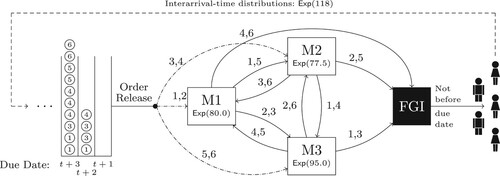
In our simulation model, depicted in Figure 1, the customers initiate the process by placing orders. This is indicated by the dashed line.

Figure 1. Production System of the Simulation Model with routing, processing time distributions and demand interarrival time distributions.

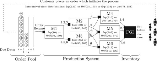
The manufacturer produces six different product types, each of which is identified by a natural number $1,2,\dots ,6$ and has a different routing through the production system. The routing setup is provided by corresponding labels of the edges. For instance, product types 1–3 are routed from machine $M1$ to machine $M2$, while the other products are transferred to machine $M3$. The production system consists of three production stages with diverging material flow and no return visits. We expect the incoming orders to be uniformly distributed among the product types. A period lasts 960 minutes ($=16$ hours) which represent two 8-hour shifts. At the beginning of each period orders can be released into the production system assuming material availability for all orders at their release date. Upon release, the orders are placed in the buffer at machine $M1$. Buffers and inventories are plotted as filled squares. Thus, each workstation is equipped with a buffer which queues the orders until processing is started. All buffers use a first-come-first-serve dispatching rule. Furthermore, each workstation processes only one order at a time and early deliveries are prohibited. Orders completed ahead if their due date remain in the finished goods inventory (FGI) until they are due and sent to the customer.

3.1.1. Processing times

The machine processing time distributions are given under the corresponding node labels of the machines. To simulate high or moderate variance the processing times for all machines are drawn from an exponential or an uniform distribution, respectively. There is one bottleneck machine ($M5$) and therefore we refer to product types 2 and 5, those routed through machine $M5$, as bottleneck products whereas products 1, 3, 4, 6 are non-bottleneck products.

3.1.2. Demand

The incoming orders are placed in the order pool with a due date slack of 10 periods, that is each order arriving within period t will be due at the end of period t + 10. The due date slack of 10 is chosen to (i) ensure sufficient time between the first occurrence of orders in the order pool and the latest possible release of orders and (ii) to have a clear cause and effect relationship between the order release decision and the cost performance in the analysis. To simulate high and moderate variability of the demand process the interarrival time between consecutive incoming orders is either drawn from an exponential ($\mathsf{E}\mathsf{x}\mathsf{p}$) or an uniform ($\mathsf{U}\mathsf{n}\mathsf{i}\mathsf{f}$) distribution, which are adjusted to yield the desired bottleneck utilisation level of either $70\mathrm{\%}$ with $\mathsf{E}\mathsf{x}\mathsf{p}\left(135\right)$ and $\mathsf{U}\mathsf{n}\mathsf{i}\mathsf{f}(95,175)$, or $80\mathrm{\%}$ with $\mathsf{E}\mathsf{x}\mathsf{p}\left(118\right)$ and $\mathsf{U}\mathsf{n}\mathsf{i}\mathsf{f}(78,158)$. These values were chosen to test the influence of the non-linear relationship between flow times and high utilisation levels.

3.1.3. Order release

Before the order release decision is made, all orders in the order pool are sorted by due date. This portrays the implementation of a sequencing rule (for a review on order pool sequencing rules see Thuerer, Stevenson, and Qu 2016). According to this sequence, orders are considered for release in the beginning of each period starting with the highest priority order.

In our model, orders are released by specifying lead times ${\mathsf{L}\mathsf{T}}_1,{\mathsf{L}\mathsf{T}}_2,\dots ,{\mathsf{L}\mathsf{T}}_6⩾1$, where the index corresponds to the product type and ${\mathsf{L}\mathsf{T}}_i\in \mathbb{N}$. By setting a lead time ${\mathsf{L}\mathsf{T}}_i$ a planned release date is computed for each order j of product type i in the order pool given by (1) $\mathsf{P}\mathsf{R}\mathsf{D}{}_j=\mathsf{D}\mathsf{D}{}_j-{\mathsf{L}\mathsf{T}}_i,$(1) where ${\mathsf{D}\mathsf{D}}_j$ denotes the due date of the order. For dynamic order releases the lead times ${\mathsf{L}\mathsf{T}}_i$ may vary from period to period, whereas in static order release methods the lead times are predetermined and fixed (Ragatz and Mabert 1988; Kim and Bobrowski 1995). For both approaches a job of product type i with lead time $\mathsf{L}\mathsf{T}{}_i$ in period t and due date ${\mathsf{D}\mathsf{D}}_j$ is released at the end of period t if and only if $t⩾\mathsf{P}\mathsf{R}\mathsf{D}{}_j$. Thus, in the dynamic setting the planned release date $\mathsf{P}\mathsf{R}\mathsf{D}{}_j$ of order j can be updated several times before it is actually released to the production system. However, once an order is released its release cannot be revoked. If there are several orders with the same due date the order release sequence is randomised. Hence, if the set lead time corresponds with the actual flow time the product is finished in the same period as it is shipped. If the lead times are set either too long or short, the order has to wait in the FGI until it is due or the order is late and backorder (BO) costs occur.

3.1.4. Costs

The cost parameters are set by assuming an increase in value from raw material (1 Dollar per order and period) to the final product (4 Dollar per order and period) and the backorder costs are set very high (16 Dollar per order and period) due to the MTO environment. All costs are assessed based on the production system state at the end of each period.

4. Lead time setting

This section describes the examined static and dynamic lead time setting approaches. For the dynamic approach we also integrate safety lead times (Enns and Suwanruji 2004, see also Haeussler, Schneckenreither, and Gerhold 2019). This addition incorporates the ratio of FGI and backorder costs into the lead time setting procedure.

4.1. Static lead times

A common approach for handling order release decisions is to use fixed (static) lead times. Therefore, we use a backward infinite loading (BIL) technique as an external benchmark, where the lead time planning parameters ${\mathsf{L}\mathsf{T}}_i$ are predetermined and constant over time.

4.2. Dynamic lead times

As stated above, a forecast-based order release model may generate an erratic order release pattern resulting in the lead time syndrome (Mather and Plossl 1978; Selcuk, Fransoo, and Kok 2006; Knollmann and Windt 2013). Thus, updating lead times may trigger the lead time syndrome as an increase of the lead time usually happens once the flow times exceeded the lead times. The increased lead times result in additional releases, i.e. a higher work-in-process level and thus over time in increased flow times, which may cause another increase of the lead time. For example, consider the flow time as the only input for forecasting the lead time. By definition the flow time can only be observed after the orders traverse the whole production system, which may take several periods. Thus, the flow times observed at a particular time were caused by an order release decision that was taken various periods in the past. Therefore, if the actual flow times exceed the lead times, the lead time may be increased accordingly. In other words, if the previously used expectations (lead times) are not matched by extended flow times the expectations are readjusted to match the measured values. However, this leads to more releases and therefore a higher work-in-process level which again increases the flow times, i.e. the effects of the lead-time syndrome occur. Thus, to prevent an uncontrolled increase of the lead times (and order releases), we enforce an upper bound on it. Based on pilot runs we set the maximum lead time to 4 periods which provides a sensible bound for the lead time of our simulation model. This approach is comparable to a backward finite loading technique (e.g. Ragatz and Mabert 1988; Bobrowski 1989; Kim and Bobrowski 1995), but instead of a maximum workload norm we set a upper bound for the lead times. By setting this upper lead time bound we enable the possibility of adaptively changing the lead times without triggering the lead time syndrome.

Figure 2 illustrates the opportunity of dynamic lead time setting, where the dashed line depicts the upper bound of the lead time. The expected minimum lead time required to fulfil all orders on time for a predetermined demand and constant maximum capacity is depicted as the solid black line. Note that the minimum required lead time to fulfil the demand of two consecutive periods are connected. For instance, in Figure 2 if a static lead time is used to release the orders, the gap between periods of the minimum required lead time consists only of the difference of orders that left the production system and the number of jobs that arrived within the upper lead time bound of the order pool between these two periods. Therefore, the size of the gaps of the required lead time is due to the variability of the demand and the manufacturing process.

Figure 2. Setting adaptive lead times.

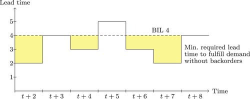
The shaded areas are the opportunities a simple reactive order release mechanism may use to reduce the flow times to save holding costs. In contrast, proactive and predictive forecasting technique may be able to shift the additional load of period t + 5 to an earlier period to prevent backorders. However, in the context of flow time forecasts this requires per order forecasts of the production system state as this allows an iterative process of releasing an order and updating the production system state by adding the released order to the corresponding queue.

In the sequel we introduce the reactive and predictive approaches analysed. The first two models stem from reactive lead time management and are based on the study of Enns and Suwanruji (2004). Afterwards the more comprehensive predictive approach using an ANN is presented.

4.2.1. Reactive lead time management: exponentially smoothed lead times

We use exponential smoothing to forecast the flow times for each product type. That is, at period t we set the lead times ${\mathsf{L}\mathsf{T}}_{i,t}=\alpha \mathsf{F}\mathsf{T}{}_{i,t}+(1-\alpha )\cdot \mathsf{L}\mathsf{T}{}_{i,t-1},$of product type i based on the forecasted flow times, where $\mathsf{F}\mathsf{T}{}_{i,t}$ is the last observed flow time for product type i and $0⩽\alpha ⩽1$ the smoothing parameter. Clearly at period t the release mechanism is initialised with ${\mathsf{L}\mathsf{T}}_i={\mathsf{L}\mathsf{T}}_{i,t}$. We test α-values of 0.1 and 0.2, as these have been shown to perform well for the given setup (Haeussler, Schneckenreither, and Gerhold 2019). To increase accuracy we forecast the flow time in minutes and round to the closest period.

4.2.2. Reactive lead time management: exponentially smoothed lead times with safety lead time

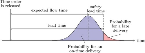
Neglecting the periodicity, and under the assumption of normally distributed deviations of the actual flow times from the lead times, the BO costs exceed the FGI costs by about the ratio of these costs. We observed deviations from this rule of thumb mainly if (i) high forecast errors occurred, and (ii) the lead times were often overridden by the upper lead time bound. Nonetheless, balancing these costs constitutes an important enhancement, especially for cost-related measures. Therefore, we developed a method to incorporate the cost ratio similar to safety stock levels in inventory systems (e.g. Silver, Pyke, and Peterson 1998). To clarify, consider Figure 3 which depicts the deviations between lead times and flow times. To match the ratio of FGI and backorder costs we select the z-quantile of the normal distribution to be at $80\mathrm{\%}$. The standard deviation used for calculating the actual safety lead time from the z-quantile is continuously updated. The additional safety lead time is then added to the forecasted flow time. A similar approach was presented by Enns and Suwanruji (2004) in a supply chain context. However, their motivation rather lies in safety stock than in balancing of cost ratios. Additionally, they simply use a constant value as opposed to deducing the safety lead time from the cost structure.

Figure 3. Safety lead time under the assumption of normally distributed deviations of the flow time forecasts.

4.2.3. Predictive lead time management via artificial neural network forecasting

In the sequel we present a predictive lead time management approach which is based on forecasts obtained using a feedforward ANN. Therefore, we first introduce the concept of feedforward ANNs, its parameterisation and the training procedure, before presenting the iterative order release algorithm.

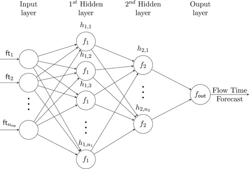
Feedforward Neural Networks. ANNs are used to approximate functions learned using sample data. In this paper we use fully-connected feedforward ANNs and thus for a more comprehensive introduction to ANNs refer to Yegnanarayana (2009). Figure 4 depicts a fully-connected feedforward ANN, in which $n_{\mathsf{i}\mathsf{n}\mathsf{p}}$ scalar input data values ${\mathsf{f}\mathsf{t}}_i$, called features, are streamed from node to node along the directed edges and thus in one direction only. Each edge represents a weight parameter $w_{i,j}$ for layer i and numbered by j. To preserve readability these are not labelled in the figure. All edges pointing to a node are linearly connected between each other. For instance node $h_{1,1}=\sum _{i=1}^{n_{\mathsf{i}\mathsf{n}\mathsf{p}}}{w}_{1,i}{\mathsf{f}\mathsf{t}}_i$. Therefore, to be able to approximate non-linear functions after each layer, except for the input layer, a non-linear (activation) function is applied to the weighted sum, i.e. instead of using the value of $h_{1,1}$ in the next layer an activation function $f_{\mathsf{1}}$ is applied and $f_{\mathsf{1}}\left(h_{1,1}\right)$ passed to the next layer.

Figure 4. The artificial neural network architecture.

Feature Extraction and Selection. As there is no standard procedure for the model building process and rules of thumb work only for special problems (Zhang 2006) we manually optimised the ANN architecture by trial-and-error and found the following as most appropriate in our setting. To reduce the complexity and computation time we developed separate flow time forecasting models for bottleneck and non-bottleneck products. That is, we train and evaluate on two separate neural networks. For both networks the input layer nodes were preselected by using the PMI-based (Sharma 2000) input selection algorithm PMIS as presented by Galelli et al. (2014). The PMIS algorithm is a filter input variable selection method which evaluates the relevance of potential input nodes based on mutual information of the input variable and the output. Additionally to account for redundancy of input variables, conditionals on any inputs that have already been selected are also evaluated.

As possible features we identified 36 production system characteristics with regard to the product type for which the forecast is demanded: The total expected processing time of the product type (P), number of operations of the product type (NO), the mean flow time of the product type (MF order), the mean flow time of the last three periods of the product type (MF LP order), the mean queuing time of the product type at each stage (MQ S1, MQ S2, MQ S3), the mean queuing time of the product type at each stage of the last three periods (MQ S1 LP, MQ S2 LP,MQ S2 LP), the mean queuing time per operation of the product type (Mq), the mean queuing time per operation of the product of the last three periods (Mq LP), the standard deviation of the flow times of the product type (SF order), the standard deviation of the product type's queueing time at each stage (SQ S1, SQ S2, SQ S3), the standard deviation of queuing time per operation of the product type (Sq), the exponentially smoothed flow time ($\alpha =0.3$ for all exponentially smoothed features) of the product type (MF EX order), the exponentially smoothed queueing time of the product type at each stage (MQ S1 EX, MQ S2 EX, MQ S3 EX), the expected total processing time of all jobs at stage 1, 2, and 3 on the product's routing (WIQ 1, WIQ 2, WIQ 3), the number of jobs in the queues of stage 1, 2 and 3 on the product's routing (JIQ 1, JIQ 2, and JIQ 3 respectively), the number of jobs in the system (JIS), the mean flow time of all jobs in the system (MF), the mean flow time of all jobs in the system of the last three periods (MF LP), the mean queuing time of all jobs in the system (MQ), the mean queuing time of all jobs in the system of the last three periods (MQ LP), the standard deviation of the flow times of all jobs in the system (SF), the standard deviation of the queuing time of all jobs in the system (SQ), the exponentially smoothed flow time of all jobs in the system (MF EX) and finally the exponentially smoothed queuing time of all jobs in the system (MQ EX).

Input Features and Network Output. The result of the feature selection provides 30 input features for both networks, cf. Table 1 where the features are sorted by their partial mutual information (PMI), of which 19 input nodes for the neural network of the bottleneck products and 21 for the non-bottleneck products are significant. Note that the jobs in queue in stage 3 are the most relevant feature for the bottleneck network, while for the non-bottleneck network the jobs in the buffer of stage 1 are the most important feature. This is due to the bottleneck machine being located at stage 3. Similarly, for both networks the exponentially smoothed overall mean queuing time (MQ,EX) is an important feature, while the exponentially smoothed mean queuing time of stage 3 (MQ,EX,S3) is much more relevant in the bottleneck network. Overall the actual numbers of jobs (JIS, JIQ1, ·) are the most relevant input features for the bottleneck product network, while ?>accumulated key figures like exponentially smoothed queuing times over the last 3 periods (e.g. MF,LP) are less important. The expected total processing times (WIQ1–WIQ3) are only a good predictor for the flow time of non-bottleneck products.

Table 1. Result of feature selection for bottleneck products (top) and non-bottleneck products (bottom), where features with $5\mathrm{\%}$-significance are printed in bold.

Feat.	JIQ3	JIS	JIQ2	JIQ1	MQ,EX	MQ,EX,S3
PMI	0.6971	0.5133	0.1019	0.07736	0.02878	0.02683
Feat.	WIQ2	MQ,EX,S1	MF,LP	MQ,LP	Mq,LP	MQ,S2
PMI	0.02608	0.02421	0.02286	0.02241	0.02215	0.02099
Feat.	MQ,S3,LP	MF,EX	MF,EX,item	MF,LP,item	MQ,EX,S2	MQ,LP,S1
PMI	0.02068	0.01691	0.01561	0.01543	0.01434	0.01393
Feat.	MQ,S2,LP	SF	Sq	SQ,S2	SQ,S3	MF
PMI	0.01239	0.01025	0.008127	0.007766	0.007221	0.005646
Feat.	MQ	SQ	Mq	MQ,S3	MF,item	SF,item
PMI	0.005482	0.005285	0.003558	0.002541	0.002164	0.001189
Feat.	JIQ1	WIQ2	WIQ3	MQ,EX	JIS	MF,EX,item
PMI	0.6484	0.1636	0.07729	0.02794	0.02545	0.02508
Feat.	MQ,LP,S1	MQ,EX,S1	MQ,LP	JIQ2	MQ,EX,S2	MF,LP
PMI	0.02494	0.02351	0.02345	0.02107	0.0201	0.01984
Feat.	MF,LP,item	JIQ3	MQ,S2	Mq,LP	MQ,S2,LP	MQ,S3,LP
PMI	0.01906	0.01785	0.01779	0.01774	0.01751	0.01674
Feat.	MQ,EX,S3	SQ,S3	MF,EX	MQ,S3	Sq	SQ,S2
PMI	0.01562	0.01392	0.01232	0.01001	0.009969	0.009168
Feat.	MF,item	SF,item	Mq	P	MF	SF
PMI	0.005694	0.004931	0.002631	−0.00143	−0.002299	−0.006629

Thus overall the mean queuing times and the flow times, i.e. current waiting times, are main factors that influence (near) future flow times. This is consistent with results of queuing theory. For instance, if we consider a single-server first-come-first-served queue with infinite buffer, i.e. a G/G/1 queue, with customers $n\in {\mathbb{N}}^{+}$ then the waiting time $w_n$ of customer n can be specified with Lindley's equations as $w_{n+1}=max(0,w_n+s_n-(a_{n+1}-a_n\left)\right)$, where $s_n$ is the service time of customer n, $a_n$ the arrival time of customer n, and $w_1=0$ (Lindley 1952 or e.g. Bambos and Walrand 1990). This means that the waiting time of the subsequent customers (orders in our context) are governed by the waiting time of the previous customers and the corresponding service times. This is represented by the WIP level as a measure for waiting times and the observed flow times, which include the service time.

As the order release problem faces sampling issues since the system's state depends on the order release quantities the training set is generated based on static order release mechanisms only. This prevents learning from data that fall into the lead time syndrome. We also performed a manual evaluation of the selected features, by comparing the forecast accuracy of using all features to the accuracy when disabling a specific feature. It resulted in dropping the mean queuing time of the job at stage 2 (MQ S2) for both networks and the standard deviation of queuing time of the product type at stage 3 (SQ S3) for the non-bottleneck products. Thus the input layers consist of 18 nodes for the neural network of the bottleneck products and 19 nodes for the non-bottleneck products. The output layers consist of a single node representing the flow time, as depicted in Figure 4.

Both input and output values are scaled to the range $[-1,1]$ using the $min$-$max$ normalisation before being fed into the network. The minimum and maximum values are computed beforehand over the training data. Thus, the output of the neural network is re-scaled to gain the estimated flow time ${\overline{FT}}_{i,\mathsf{p}\mathsf{s}\mathsf{s}}$ of product type i and under the current production system state $\mathsf{p}\mathsf{s}\mathsf{s}$. The lead time ${\mathsf{L}\mathsf{T}}_{i,\mathsf{p}\mathsf{s}\mathsf{s}}$ is calculated by adding the safety lead time as described in Section 4.2.2: ${\mathsf{L}\mathsf{T}}_{i,\mathsf{p}\mathsf{s}\mathsf{s}}={\overline{FT}}_{i,\mathsf{p}\mathsf{s}\mathsf{s}}+\mathsf{L}\mathsf{T}{}_{i,\mathsf{s}\mathsf{a}\mathsf{f}\mathsf{e}\mathsf{t}\mathsf{y}}.$Therefore, the release mechanism is initialised with ${\mathsf{L}\mathsf{T}}_i={\mathsf{L}\mathsf{T}}_{i,\mathsf{p}\mathsf{s}\mathsf{s}}$, whenever $\mathsf{p}\mathsf{s}\mathsf{s}$ is the currently observable production system state.

Hidden Layers and Activation Functions. For both networks there are two hidden layers, where the first consists of 28 nodes and the second of 14 nodes. We arrived at this setup by repeatedly training different network architectures. We started with the hidden layers each containing 1.5 times the sum of input and output nodes, i.e. 3, and then iteratively reduced the number of nodes while searching for the smallest mean squared error (MSE) of the validation set (20% of the training data). After each layer, except the input layer, the commonly used activation function $\mathsf{R}\mathsf{e}\mathsf{L}\mathsf{U}$ (rectified linear unit) is applied, that is $f_1=f_2=f_{\mathsf{o}\mathsf{u}\mathsf{t}}=\mathsf{R}\mathsf{e}\mathsf{L}\mathsf{U}$. This allows the neural network to disable some neurons on certain inputs leading to sparse networks, similar to the hypothesised sparsity of brain structures (Glorot, Bordes, and Bengio 2011).

Training. As ANNs are a data-driven approach a data set must be generated and trained before the neural network returns sensible output. For this data-generation process we used overall about 400 thousand orders, where the orders were released using BIL with lead times 1−5 (see Equation (1(1) $\mathsf{P}\mathsf{R}\mathsf{D}{}_j=\mathsf{D}\mathsf{D}{}_j-{\mathsf{L}\mathsf{T}}_i,$(1) )). The generated data was randomised and split into batches of 256 orders to smooth the learning process. As recommended by Zhang (2006) 80% of the data was used for training and $20\mathrm{\%}$ as a validation set, where we dropped the fine-tuning portion, as we were able to regenerate data from the simulation. Other batch-sizes (64, 128, 512) were evaluated but discarded due to worse estimates (higher MSEs). To obtain an acceptable mean squared error of around $3.5\mathrm{\%}$ on the validation set we cycled the training process up to 5 times. For training the gradients based on the squared loss are propagated back using Adagrad (Duchi, Elad, and Yoram 2011) with a learning rate of 0.01, where again we tested different values ($0.001,0.005,0.01$) and chose the best performing one. We also tested the RMSProp (Tieleman and Hinton 2012) backpropagation algorithm as optimiser, but favoured Adagrad due to better performance.

Order Release. As this forecasting technique is order-based and incorporates the status of the shop floor we iteratively forecast the flow time of orders and release them accordingly. This allows us to anticipate future backorders and, avoid them by releasing orders earlier. According to the reference framework of Bergamaschi et al. (1997), the procedure is similar to a time bucketing approach (e.g. Bobrowski 1989) with an extended schedule visibility and works as follows, where t is initialised as current period:

Step 0	Forecast the flow time of all orders in the order pool, one at a time, starting with the order having the earliest due date and release all orders j with ${\mathsf{P}\mathsf{R}\mathsf{D}}_j⩽t$. Initialise the time-bucketing algorithm with the current production system state, unmark all orders remaining in the order pool and set $t^{\prime }=t+1$.
Step 1	For each unmarked order j in the order pool, starting with the order having the earliest due date, forecast the flow time, where the marked orders are added to the WIP level of the orders' gateway work centre. Then by calculating the corresponding lead time infer its planned release date ${\mathsf{P}\mathsf{R}\mathsf{D}}_j$: if ${\mathsf{P}\mathsf{R}\mathsf{D}}_j<t^{\prime }$: Release the order with the earlierst due date of the order pool and remove order j from the simulation, further unmark all orders, set $t^{\prime }=t+1$ and go to Step 1. if ${\mathsf{P}\mathsf{R}\mathsf{D}}_j=t^{\prime }$: Mark the order and continue the loop. if ${\mathsf{P}\mathsf{R}\mathsf{D}}_j>t^{\prime }$: Continue the loop.
Step 2	Increment $t^{\prime }$ by 1, reduce the WIP level of all stages by the expected system output and go to Step 1 until all orders of the order pool are marked.

This algorithm continuously loops through the orders of the order pool, evaluates the expected planned release date for each order and marks orders to keep track of orders that are expected to be completed on time. If an order is expected to arrive at the inventory after its due date, the algorithm is designed to release orders earlier, i.e. it shifts the expected additional load of later periods to the previous periods. The loop halts if, based on the forecasts generated by the ANN, all orders are expected to arrive on time.

Example 4.1

For simplicity consider a single product type (product type 1), suppose the current period is t, and that there are no orders in the bucket with due date t + 1 (bucket A), 4 orders in the bucket with t + 2 (bucket B) and 10 orders in the bucket t + 3 (bucket C) as in Figure 1. Furthermore, let the lead time ${\mathsf{L}\mathsf{T}}_1=1$ for all orders.

Then in the current period there is nothing to be released as all orders have ${\mathsf{P}\mathsf{R}\mathsf{D}}_j⩾t+1$. Thus, the time-bucketing algorithm starts with no released orders in the current period. In the first iteration $t^{\prime }=t+1$ the algorithm marks the orders of bucket B one after the other. After processing bucket B assume a lead time update to ${\mathsf{L}\mathsf{T}}_{1,\mathsf{p}\mathsf{s}\mathsf{s}}=2$ due to the additional load in the buffer of M1. Then after marking all jobs of bucket B it continues with checking the orders of bucket C. It may happen that after marking some but not all orders of bucket C the estimated flow time again increases due to the additionally marked orders. In this case the next job will have a planned release date of $t^{\prime }-1$, thus another order of bucket B is released at the current period t, and the process restarts, until all orders of the order pool are expected to be on time.

5. Results

This section presents the results of the forecast accuracy and proofs the viability of dynamic order release methods. The length of each simulation run to evaluate the performance was 8000 periods including a warm-up period of 1000 periods. Each simulated scenario was run for 30 replications and their means are reported. Welch's procedure was applied to approximate the length of the warm-up period (see Law and Kelton 2000).

5.1. Forecast accuracy

The forecast accuracy is measured as average absolute deviation over all products between forecasted and actual flow times (given in minutes). Figure 5 depicts the forecast accuracy for all tested scenarios. For brevity, we use a triple to denote each scenario: The first component corresponds to either 70% or 80% bottleneck utilisation, the second denotes the interarrival times of the demand, and the third, $\mathsf{E}\mathsf{x}\mathsf{p}$ or $\mathsf{U}\mathsf{n}\mathsf{i}\mathsf{f}$, represents the distribution for the processing times.

Figure 5. Flow time forecast accuracy of all products for all scenarios.

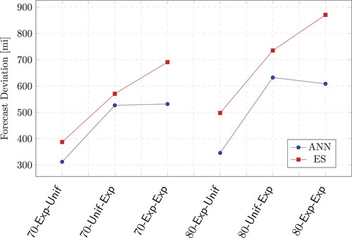
Figure 5 reveals that the process time variability has the biggest impact on forecast accuracy, since the forecast deviations increase from cases with uniformly to exponentially distributed processing times.

Overall, the forecasts of the artificial neural network are more accurate than with the exponential smoothing technique for all scenarios and the relative advantage increases from 70% to 80% utilisation and is biggest for the 80-$\mathsf{E}\mathsf{x}\mathsf{p}$-$\mathsf{E}\mathsf{x}\mathsf{p}$ scenario.

5.2. Computational experiments

Table 2 shows the results of the evaluations for an utilisation level of 70%. The first column denotes the tested order release approaches, namely (i) the static lead time approach (denoted as $\mathsf{B}\mathsf{I}\mathsf{L}$), (ii) the reactive approaches ${\mathsf{E}\mathsf{S}\mathsf{S}\mathsf{L}\mathsf{T}}_{0.1}$ and ${\mathsf{E}\mathsf{S}\mathsf{S}\mathsf{L}\mathsf{T}}_{0.2}$ with safety lead time where the corresponding α-value is given as index, and (iii) the predictive $\mathsf{A}\mathsf{N}\mathsf{N}$ approach using the artificial neural network. Column two to six depict the cost-based performance measures in ${10}^3$ Dollars: the costs for held WIP (WIPC), finished goods inventory costs (FGIC), backorder costs (BOC), timing costs which is the sum of FGIC and BOC and sum over all costs (SUM). The mean of all values are compared for all algorithms at a significance level of p = 0.05 using a Wilcoxon/Mann–Whitney-U Test. The values marked with an asterisk are not significantly different from the best performing model. Finally, the last column shows the service level denoted as SL(%) reached in percent.

Table 2. Results for a bottleneck utilisation of 70%.

70-$\mathsf{E}\mathsf{x}\mathsf{p}$-$\mathsf{U}\mathsf{n}\mathsf{i}\mathsf{f}$	WIPC	FGIC	BOC	FGIC+BOC	SUM	SL(%)
${\mathsf{E}\mathsf{S}\mathsf{S}\mathsf{L}\mathsf{T}}_{0.1}$	34.2	47.2	151.8	199.0	233.2	82.5%
$\mathsf{A}\mathsf{N}\mathsf{N}$	48.5	187.2	10.8	198.0${}^{\ast }$	246.4	98.8%
${\mathsf{E}\mathsf{S}\mathsf{S}\mathsf{L}\mathsf{T}}_{0.2}$	35.4	39.0	184.3	223.3	258.6	78.7%
$\mathsf{B}\mathsf{I}\mathsf{L}$	29.3	480.2	0.5	480.7	510.0	99.9%
70-$\mathsf{U}\mathsf{n}\mathsf{i}\mathsf{f}$-$\mathsf{E}\mathsf{x}\mathsf{p}$	WIPC	FGIC	BOC	FGIC+BOC	SUM	SL(%)
${\mathsf{E}\mathsf{S}\mathsf{S}\mathsf{L}\mathsf{T}}_{0.1}$	45.3	75.6	177.5	253.2	298.4	82.7%
$\mathsf{A}\mathsf{N}\mathsf{N}$	67.5	180.7	60.2	240.9	308.4	94.3%
${\mathsf{E}\mathsf{S}\mathsf{S}\mathsf{L}\mathsf{T}}_{0.2}$	48.3	73.1	207.0	280.1	328.4	79.9%
$\mathsf{B}\mathsf{I}\mathsf{L}$	40.1	439.7	11.1	450.8	490.8	99.1%
70-$\mathsf{E}\mathsf{x}\mathsf{p}$-$\mathsf{E}\mathsf{x}\mathsf{p}$	WIPC	FGIC	BOC	FGIC+BOC	SUM	SL(%)
$\mathsf{A}\mathsf{N}\mathsf{N}$	76.6	169.7	92.5	262.2	338.8	91.6%
${\mathsf{E}\mathsf{S}\mathsf{S}\mathsf{L}\mathsf{T}}_{0.1}$	55.3	89.1	228.0	317.2	372.5	79.5%
${\mathsf{E}\mathsf{S}\mathsf{S}\mathsf{L}\mathsf{T}}_{0.2}$	57.9	88.7	242.5	331.2	398.1	78.5%
$\mathsf{B}\mathsf{I}\mathsf{L}$	48.6	409.0	24.2	433.2	481.8	98.0%

As one can see, for an utilisation level of $70\mathrm{\%}$, ${\mathsf{E}\mathsf{S}\mathsf{S}\mathsf{L}\mathsf{T}}_{0.1}$ performs best regarding the total costs measure for two out of three scenarios. However, the differences between the two best performing approaches (${\mathsf{E}\mathsf{S}\mathsf{S}\mathsf{L}\mathsf{T}}_{0.1}$ and $\mathsf{A}\mathsf{N}\mathsf{N}$) is rather small (13.3 for 70-$\mathsf{E}\mathsf{x}\mathsf{p}$-$\mathsf{U}\mathsf{n}\mathsf{i}\mathsf{f}$ and 9.9 for 70-$\mathsf{U}\mathsf{n}\mathsf{i}\mathsf{f}$-$\mathsf{E}\mathsf{x}\mathsf{p}$) but significant. The main difference between these two approaches is that the $\mathsf{A}\mathsf{N}\mathsf{N}$ yields the highest WIP costs of all tested approaches which we attribute to its strong emphasis on timing performance. In this regard, the $\mathsf{A}\mathsf{N}\mathsf{N}$ model performs best (lowest FGI+BOC costs for all scenarios) where since it yields the second highest service level together with a quite balanced ratio between FGI and BO costs for all scenarios. This suggests that the proposed method can be further refined by reducing the WIP costs (for a first step into this direction see Section 5.3.4 below). However, additionally optimising in regard to this cost is out of the scope of this paper and thus left as future work.

Table 3 depicts the results for an utilisation level of 80%. Similar to the results presented above, the $\mathsf{A}\mathsf{N}\mathsf{N}$ model yields the highest WIP costs for all scenarios. Due to this, $\mathsf{A}\mathsf{N}\mathsf{N}$ performs second-best in the scenario with exponentially distributed interarrival-times and uniform processing times. Here the ${\mathsf{E}\mathsf{S}\mathsf{S}\mathsf{L}\mathsf{T}}_{0.1}$ model has the lowest overall costs which is mainly due to the much lower WIP costs which are only 62.9% of the WIPC for the $\mathsf{A}\mathsf{N}\mathsf{N}$ model. For the other two scenarios (80-$\mathsf{U}\mathsf{n}\mathsf{i}\mathsf{f}$-$\mathsf{E}\mathsf{x}\mathsf{p}$ and 80-$\mathsf{E}\mathsf{x}\mathsf{p}$-$\mathsf{E}\mathsf{x}\mathsf{p}$) the $\mathsf{A}\mathsf{N}\mathsf{N}$ model performs best. It is noteworthy that in the case of exponentially distributed interarrival- and processing times (80-$\mathsf{E}\mathsf{x}\mathsf{p}$-$\mathsf{E}\mathsf{x}\mathsf{p}$) the static order release model ($\mathsf{B}\mathsf{I}\mathsf{L}$) yields the third-best performance.

Table 3. Results for a bottleneck utilisation of 80%.

80-$\mathsf{E}\mathsf{x}\mathsf{p}$-$\mathsf{U}\mathsf{n}\mathsf{i}\mathsf{f}$	WIPC	FGIC	BOC	FGIC+BOC	SUM	SL(%)
${\mathsf{E}\mathsf{S}\mathsf{S}\mathsf{L}\mathsf{T}}_{0.1}$	55.4	71.1	170.6	241.8	297.2	84.7%
$\mathsf{A}\mathsf{N}\mathsf{N}$	88.1	165.0	69.2	234.1	322.2	93.9%
${\mathsf{E}\mathsf{S}\mathsf{S}\mathsf{L}\mathsf{T}}_{0.2}$	59.1	64.5	211.4	275.9	335.0	81.1%
$\mathsf{B}\mathsf{I}\mathsf{L}$	45.9	501.8	7.8	509.6	555.5	99.4%
80-$\mathsf{U}\mathsf{n}\mathsf{i}\mathsf{f}$-$\mathsf{E}\mathsf{x}\mathsf{p}$	WIPC	FGIC	BOC	FGIC+BOC	SUM	SL(%)
$\mathsf{A}\mathsf{N}\mathsf{N}$	109.2	211.2	141.9	353.0	462.2	90.3%
${\mathsf{E}\mathsf{S}\mathsf{S}\mathsf{L}\mathsf{T}}_{0.1}$	79.5	103.0	311.7	414.7	494.3	77.3%
${\mathsf{E}\mathsf{S}\mathsf{S}\mathsf{L}\mathsf{T}}_{0.2}$	83.1	96.6	333.7	430.3	513.3	76.0%
$\mathsf{B}\mathsf{I}\mathsf{L}$	65.4	436.2	57.6	493.8	559.2	96.5%
80-$\mathsf{E}\mathsf{x}\mathsf{p}$-$\mathsf{E}\mathsf{x}\mathsf{p}$	WIPC	FGIC	BOC	FGIC+BOC	SUM	SL(%)
$\mathsf{A}\mathsf{N}\mathsf{N}$	116.3	188.0	220.0	407.9	524.3	86.0%
${\mathsf{E}\mathsf{S}\mathsf{S}\mathsf{L}\mathsf{T}}_{0.1}$	93.0	136.9	367.9	504.8	597.8	76.2%
$\mathsf{B}\mathsf{I}\mathsf{L}$	78.4	396.0	131.8	527.8	606.2	94.0%
${\mathsf{E}\mathsf{S}\mathsf{S}\mathsf{L}\mathsf{T}}_{0.2}$	98.4	121.6	411.9	533.5	631.8	73.9%

5.3. Sensitivity analysis

In this subsection, the different order release approaches are analysed in multiple settings. More precisely, we test the influence of a job shop production environment, the safety lead time, different cost parameters and limiting the release quantity. We use the 80-$\mathsf{E}\mathsf{x}\mathsf{p}$-$\mathsf{E}\mathsf{x}\mathsf{p}$ scenario as a base treatment and compare the cost performance between $\mathsf{A}\mathsf{N}\mathsf{N}$, ${\mathsf{E}\mathsf{S}\mathsf{S}\mathsf{L}\mathsf{T}}_{0.1}$, ${\mathsf{E}\mathsf{S}\mathsf{S}\mathsf{L}\mathsf{T}}_{0.2}$ and $\mathsf{B}\mathsf{I}\mathsf{L}$.

5.3.1. Job shop production environment

In order to guarantee comparability to the tested flow shop we use a restricted job shop (as defined by Oosterman, Land, and Gaalman 2000) with three machines where six products are processed. All products visit all work centres, but the sequence of the visits is different for each product (see Figure 6). The interarrival time of orders at the job shop are equal to the interarrival times for the flow shop which yields an average utilisation of 80% and there is one bottleneck work centre (M3).

Figure 6. Job Shop Simulation Model with routing, processing time distributions and demand interarrival time distributions.

Regarding the forecast accuracy the $\mathsf{A}\mathsf{N}\mathsf{N}$ yields an average forecast deviation of 482.4 compared to 532.13 with the exponential smoothing technique. This means that, similar to above (see Figure 5), the forecasts of the $\mathsf{A}\mathsf{N}\mathsf{N}$ are more accurate, although the relative difference is smaller for the job shop.

Table 4 shows the cost performance of the tested order release models for the job shop environment for exponential interarrival and processing times.

Table 4. Results for job shop production environment.

80-$\mathsf{E}\mathsf{x}\mathsf{p}$-$\mathsf{E}\mathsf{x}\mathsf{p}$	WIPC	FGIC	BOC	FGIC+BOC	SUM	SL(%)
$\mathsf{A}\mathsf{N}\mathsf{N}$	77.2	189.8	95.5	285.3	362.6	91.1%
${\mathsf{E}\mathsf{S}\mathsf{S}\mathsf{L}\mathsf{T}}_{0.1}$	45.2	88.7	232.6	321.3	366.5${}^{\ast }$	79.4%
${\mathsf{E}\mathsf{S}\mathsf{S}\mathsf{L}\mathsf{T}}_{0.2}$	52.2	80.9	274.2	355.1	407.3	76.0%
$\mathsf{B}\mathsf{I}\mathsf{L}$	34.5	545.2	2.5	547.7	582.2	99.8%

The general insights from above hold here as well: (i) The $\mathsf{A}\mathsf{N}\mathsf{N}$ approach yields the highest WIP costs, i.e. 170% in comparison to ${\mathsf{E}\mathsf{S}\mathsf{S}\mathsf{L}\mathsf{T}}_{0.1}$ and (ii) the lowest timing costs (FGI+BOC) and (iii) the $\mathsf{A}\mathsf{N}\mathsf{N}$ model yields the lowest total costs, although, for the job shop, there is no significant difference from the ${\mathsf{E}\mathsf{S}\mathsf{S}\mathsf{L}\mathsf{T}}_{0.1}$ model¹.

5.3.2. Safety lead time

Table 5 compares the order release methods in regard to the safety lead time. In the top part of the Table, all methods are configured to use the safety lead times as specified in Subsection 4.2.2, whereas the bottom part of the table shows the results for the base treatment (80-$\mathsf{E}\mathsf{x}\mathsf{p}$-$\mathsf{E}\mathsf{x}\mathsf{p}$), but with safety lead times disabled. For all ‘no safety lead time’ scenarios we test whether the results are significantly different from to the initial results at a significance level of p = 0.05 using a Wilcoxon/Mann–Whitney-U Test. Thus, the values marked with an asterisk are not significantly different from the corresponding ‘safety lead time’ values.

Table 5. Results for 80-$\mathsf{E}\mathsf{x}\mathsf{p}$-$\mathsf{E}\mathsf{x}\mathsf{p}$ with (top) and without safety lead times (bottom).

Safety lead time	WIPC	FGIC	BOC	FGIC+BOC	SUM	SL(%)
$\mathsf{A}\mathsf{N}\mathsf{N}$	116.3	188.0	220.0	407.9	524.3	86.0%
${\mathsf{E}\mathsf{S}\mathsf{S}\mathsf{L}\mathsf{T}}_{0.1}$	93.0	136.9	367.9	504.8	597.8	76.2%
${\mathsf{E}\mathsf{S}\mathsf{S}\mathsf{L}\mathsf{T}}_{0.2}$	98.4	121.6	411.9	533.5	631.8	73.9%
No Safety lead time	WIPC	FGIC	BOC	FGIC+BOC	SUM	SL(%)
${\mathsf{A}\mathsf{N}\mathsf{N}}_{-}{\mathsf{n}\mathsf{o}}_{-}\mathsf{s}\mathsf{a}\mathsf{f}\mathsf{e}\mathsf{t}\mathsf{y}$	124.9	168.0	315.2	483.2	608.2	79.9%
${\mathsf{E}\mathsf{S}}_{0.1}$	97.6	37.2	896.7	933.8	1031.4	43.4%
${\mathsf{E}\mathsf{S}}_{0.2}$	103.3	31.2	957.1	988.3	1091.6	40.2%

One can see that setting the safety lead time has a positive effect on the total costs and the service level of all treatments. The latter increases for all methods and the total costs decrease by 83.9, 433.6 and 459.8 for $\mathsf{A}\mathsf{N}\mathsf{N}$, ${\mathsf{E}\mathsf{S}\mathsf{S}\mathsf{L}\mathsf{T}}_{0.1}$, and ${\mathsf{E}\mathsf{S}\mathsf{S}\mathsf{L}\mathsf{T}}_{0.2}$ respectively. Thus, exponential smoothing benefits more from safety lead times than $\mathsf{A}\mathsf{N}\mathsf{N}$, which is due to the worse estimates and reactive behaviour. Finally, the comparative advantage of ${\mathsf{A}\mathsf{N}\mathsf{N}}_{-}{\mathsf{n}\mathsf{o}}_{-}\mathsf{s}\mathsf{a}\mathsf{f}\mathsf{e}\mathsf{t}\mathsf{y}$ over the two exponential smoothing approaches (${\mathsf{E}\mathsf{S}}_{0.1}$ and ${\mathsf{E}\mathsf{S}}_{0.2}$) remains unchanged where $\mathsf{A}\mathsf{N}\mathsf{N}\mathsf{\_}\mathsf{n}\mathsf{o}\mathsf{\_}\mathsf{s}\mathsf{a}\mathsf{f}\mathsf{e}\mathsf{t}\mathsf{y}$ yields the highest WIPC (128.0% of ${\mathsf{E}\mathsf{S}}_{0.1}$) better timing (FGIC+BOC) and total costs. However, the relative advantage increased vastly: $\mathsf{A}\mathsf{N}\mathsf{N}\mathsf{\_}\mathsf{n}\mathsf{o}\mathsf{\_}\mathsf{s}\mathsf{a}\mathsf{f}\mathsf{e}\mathsf{t}\mathsf{y}$ results in 51.7% of the timing and 59.0% of the total costs compared to ${\mathsf{E}\mathsf{S}}_{0.1}$.

5.3.3. Cost parameters

To investigate the behaviour under different cost structures, which alter the safety lead times by changing the used z-values (cf. Section 4.2.2), Table 6 establishes a sensitivity analysis for all treatments with modified cost ratios of 1:9 and 1:19 in regard to FGIC and BOC as supposed to 1:4 in the initial experimental design, where the WIP costs remain unchanged (see Table 3). The mean of all values are compared for all algorithms at a significance level of p = 0.05 using a Wilcoxon/Mann–Whitney-U Test. The values marked with an asterisk are not significantly different from the best performing model.

Table 6. Sensitivity analysis for modified cost ratios of FGIC and BOC.

80-$\mathsf{E}\mathsf{x}\mathsf{p}$-$\mathsf{U}\mathsf{n}\mathsf{i}\mathsf{f}$ 1:9	WIPC	FGIC	BOC	FGIC+BOC	SUM	SL(%)
$\mathsf{A}\mathsf{N}\mathsf{N}$	83.6	188.2	106.3	294.6	378.2	95.9%
${\mathsf{E}\mathsf{S}\mathsf{S}\mathsf{L}\mathsf{T}}_{0.1}$	58.3	97.5	339.0	436.5	494.8	86.7%
${\mathsf{E}\mathsf{S}\mathsf{S}\mathsf{L}\mathsf{T}}_{0.2}$	61.4	100.8	352.9	453.7	515.1	86.2%
80-$\mathsf{E}\mathsf{x}\mathsf{p}$-$\mathsf{U}\mathsf{n}\mathsf{i}\mathsf{f}$ 1:19	WIPC	FGIC	BOC	FGIC+BOC	SUM	SL(%)
$\mathsf{A}\mathsf{N}\mathsf{N}$	81.1	212.1	168.3	380.4	461.4	96.9%
${\mathsf{E}\mathsf{S}\mathsf{S}\mathsf{L}\mathsf{T}}_{0.1}$	59.1	163.5	480.8	644.3	703.4	90.9%
${\mathsf{E}\mathsf{S}\mathsf{S}\mathsf{L}\mathsf{T}}_{0.2}$	61.6	155.5	505.1	660.6	722.2	90.6%
80-$\mathsf{U}\mathsf{n}\mathsf{i}\mathsf{f}$-$\mathsf{E}\mathsf{x}\mathsf{p}$ 1:9	WIPC	FGIC	BOC	FGIC+BOC	SUM	SL(%)
$\mathsf{A}\mathsf{N}\mathsf{N}$	101.9	262.9	227.0	489.9	591.8	93.1%
${\mathsf{E}\mathsf{S}\mathsf{S}\mathsf{L}\mathsf{T}}_{0.1}$	77.1	200.4	397.0	597.3	674.4	87.8%
${\mathsf{E}\mathsf{S}\mathsf{S}\mathsf{L}\mathsf{T}}_{0.2}$	81.9	178.2	472.6	650.7	732.6	85.5%
80-$\mathsf{U}\mathsf{n}\mathsf{i}\mathsf{f}$-$\mathsf{E}\mathsf{x}\mathsf{p}$ 1:19	WIPC	FGIC	BOC	FGIC+BOC	SUM	SL(%)
$\mathsf{A}\mathsf{N}\mathsf{N}$	96.8	294.2	441.2	735.4	832.2	94.0%
${\mathsf{E}\mathsf{S}\mathsf{S}\mathsf{L}\mathsf{T}}_{0.1}$	74.8	244.5	583.9	828.4	903.1	91.8%
${\mathsf{E}\mathsf{S}\mathsf{S}\mathsf{L}\mathsf{T}}_{0.2}$	78.4	233.5	677.5	911.0	989.4	90.7%
80-$\mathsf{E}\mathsf{x}\mathsf{p}$-$\mathsf{E}\mathsf{x}\mathsf{p}$ 1:9	WIPC	FGIC	BOC	FGIC+BOC	SUM	SL(%)
$\mathsf{A}\mathsf{N}\mathsf{N}$	109.9	238.1	398.5	636.6	746.4	89.2%
${\mathsf{E}\mathsf{S}\mathsf{S}\mathsf{L}\mathsf{T}}_{0.1}$	87.3	221.7	459.8	681.5	768.7${}^{\ast }$	87.3%
${\mathsf{E}\mathsf{S}\mathsf{S}\mathsf{L}\mathsf{T}}_{0.2}$	91.7	201.6	536.9	738.5	830.2	85.2%
80-$\mathsf{E}\mathsf{x}\mathsf{p}$-$\mathsf{E}\mathsf{x}\mathsf{p}$ 1:19	WIPC	FGIC	BOC	FGIC+BOC	SUM	SL(%)
$\mathsf{A}\mathsf{N}\mathsf{N}$	105.1	281.5	733.5	1015.0	1120.2	90.9%
${\mathsf{E}\mathsf{S}\mathsf{S}\mathsf{L}\mathsf{T}}_{0.1}$	88.2	270.9	816.7	1087.6	1175.8	89.4%
${\mathsf{E}\mathsf{S}\mathsf{S}\mathsf{L}\mathsf{T}}_{0.2}$	91.5	253.2	935.6	1188.8	1280.3	88.2%

The results with altered cost parameters show that the comparative advantage of our proposed $\mathsf{A}\mathsf{N}\mathsf{N}$ remains unchanged: Again the WIPC are the highest, the timing and total costs (FGI+BOC) are the lowest for the $\mathsf{A}\mathsf{N}\mathsf{N}$ approach for all scenarios. Additionally, the cost ratios can be interpreted as target service levels such that a cost ratio of 1:9 and 1:19 represent a target value of 90% and 95%. As can be seen in Table 6 our proposed $\mathsf{A}\mathsf{N}\mathsf{N}$ approach meets that target in five out of eight cases, while in two cases the target service level was only missed by less than 1.1% (80-$\mathsf{U}\mathsf{n}\mathsf{i}\mathsf{f}$-$\mathsf{E}\mathsf{x}\mathsf{p}$ 1:19 and 80-$\mathsf{E}\mathsf{x}\mathsf{p}$-$\mathsf{E}\mathsf{x}\mathsf{p}$ 1:9) and in one case (80-$\mathsf{E}\mathsf{x}\mathsf{p}$-$\mathsf{E}\mathsf{x}\mathsf{p}$ 1:19) by 4.1%. The exponential smoothing approaches never reach the target service level. The conclusion from this sensitivity analysis is twofold: First, the safety time procedure works quite well for our predictive order release approach. Second from a practical point of view, it eases the applicability of our approach since the safety time procedure is easy to understand and well known from inventory control literature.

5.3.4. Limiting the release quantities

Since in all of the above tested scenarios our proposed predictive order release approach ($\mathsf{A}\mathsf{N}\mathsf{N}$) yields the highest WIP costs, we also analyse the potential of limiting the release quantity. Therefore, we introduce a limit to the jobs in the queue of the gateway work centre. This limit is checked after each released order, if the limit is reached no more orders are released and thus remain in the order pool until the next period.

Table 7 is divided into four parts where, for convenience, the top part depicts the initial results without limit (denoted as ‘no limit’) and the second to the lowest part present the cost performance for simulation runs with limits of 10, 12 and 14 orders (recall the expected arrival of just above 8 orders per period). For all scenarios with limited release quantities, we test whether the results are significant different to the initial results at a significance level of p = 0.05 using a Wilcoxon/Mann–Whitney-U Test. Thus, the values marked with an asterisk are not significantly different from the corresponding ‘no limit’ values.

Table 7. Results for 80-$\mathsf{E}\mathsf{x}\mathsf{p}$-$\mathsf{E}\mathsf{x}\mathsf{p}$ with limited release quantity.

No limit	WIPC	FGIC	BOC	FGIC+BOC	SUM	SL(%)
$\mathsf{A}\mathsf{N}\mathsf{N}$	116.3	188.0	220.0	407.9	524.3	86.0%
${\mathsf{E}\mathsf{S}\mathsf{S}\mathsf{L}\mathsf{T}}_{0.1}$	93.0	136.9	367.9	504.8	597.8	76.2%
${\mathsf{E}\mathsf{S}\mathsf{S}\mathsf{L}\mathsf{T}}_{0.2}$	98.4	121.6	411.9	533.5	631.8	73.9%
Limit 10	WIPC	FGIC	BOC	FGIC+BOC	SUM	SL(%)
$\mathsf{A}\mathsf{N}\mathsf{N}$	100.3	157.2	268.0	425.2	525.5${}^{\ast }$	82.7%
${\mathsf{E}\mathsf{S}\mathsf{S}\mathsf{L}\mathsf{T}}_{0.1}$	87.2	111.0	434.2	545.3	632.5	71.6%
${\mathsf{E}\mathsf{S}\mathsf{S}\mathsf{L}\mathsf{T}}_{0.2}$	92.4	98.3	491.6	589.9	682.3	69.0%
Limit 12	WIPC	FGIC	BOC	FGIC+BOC	SUM	SL(%)
$\mathsf{A}\mathsf{N}\mathsf{N}$	102.9	174.1	216.9${}^{\ast }$	391.0	493.9	85.4%
${\mathsf{E}\mathsf{S}\mathsf{S}\mathsf{L}\mathsf{T}}_{0.1}$	91.7${}^{\ast }$	125.1	402.5	527.6	619.3	74.1%
${\mathsf{E}\mathsf{S}\mathsf{S}\mathsf{L}\mathsf{T}}_{0.2}$	95.2	112.8	435.1	547.9	643.0${}^{\ast }$	72.1%
Limit 14	WIPC	FGIC	BOC	FGIC+BOC	SUM	SL(%)
$\mathsf{A}\mathsf{N}\mathsf{N}$	108.3	180.4	225.4${}^{\ast }$	405.8${}^{\ast }$	514.1${}^{\ast }$	85.6%
${\mathsf{E}\mathsf{S}\mathsf{S}\mathsf{L}\mathsf{T}}_{0.1}$	92.3${}^{\ast }$	132.8	378.7	511.5${}^{\ast }$	603.7${}^{\ast }$	75.5%
${\mathsf{E}\mathsf{S}\mathsf{S}\mathsf{L}\mathsf{T}}_{0.2}$	95.9	114.4	421.1${}^{\ast }$	535.4${}^{\ast }$	631.4${}^{\ast }$	72.8%

As expected, the introduction of a release limit reduces the service level for all scenarios. Furthermore, the order release approaches using exponential smoothing do not benefit from this extension. Regarding the $\mathsf{A}\mathsf{N}\mathsf{N}$ approach one can see that the limits have an influence on its performance: The WIPC can be decreased for all scenarios and for a limit of 12 orders also the timing and total costs are significantly lower in comparison to the ‘no limit’ scenario. Thus, we conclude that this rather simple extension highlights the potential of combining the $\mathsf{A}\mathsf{N}\mathsf{N}$ approach with more sophisticated workload control mechanisms (e.g. Yan et al. 2016; Thuerer, Stevenson, and Qu 2016; Hutter, Haeussler, and Missbauer 2018).

5.4. Managerial implications

The $\mathsf{A}\mathsf{N}\mathsf{N}$ model yields high quality flow time estimates which can help decision makers to adapt lead times dynamically. Furthermore, if the resource configuration remains unchanged for a relatively long period, an order release model using $\mathsf{A}\mathsf{N}\mathsf{N}$-based flow time forecasts may be a viable alternative to existing approaches. Therefore, the main practical relevance of this research is that $\mathsf{A}\mathsf{N}\mathsf{N}$ models can support planners to make refined order release decisions.

Thus, we encourage companies to use ANN based flow time forecasts to reduce production costs and preserve marketability. The presented examples of making order release decisions based on these forecasts show that, especially in cases with high processing times variability, our predictive model outperforms static and reactive lead time approaches. For instance, the $\mathsf{A}\mathsf{N}\mathsf{N}$ model reduced the total aggregated costs to about $70.3\mathrm{\%}$ as compared to a model that uses static lead times in the case of moderate utilisation ($70\mathrm{\%}$) and high variability in demand and processing times (see Table 2). Therefore, we suggest to implement the presented predictive approach in both, flow shops and job shops.

6. Conclusion

An essential task in manufacturing planning and control is to determine when to release orders to the shop floor. One key parameter is the lead time, which is defined as the planned time that elapses between the release of an order and its completion. Lead times are normally determined based on the actual duration that an order takes to traverse through the production system (flow times). Traditional order release models assume static lead times, although they should be set dynamically to reflect the dynamic operational characteristics of the system. Therefore, this paper presents a flow time estimation procedure to set lead times dynamically using an artificial neural network. We use a simulation of a three-stage flow-shop and compare the performance to other forecast-based order release models from literature and measure the performance by comparing the forecast accuracy and the aggregate holding and backorder costs. The results show that regarding the forecast accuracy, the machine learning model outperform the approach using exponential smoothing in all scenarios with high processing time variability and in cases with high utilisation. With regard to the cost performance, our proposed order release model perform best for all but one scenario with 80% utilisation (exponentially distributed interarrival times and uniform processing times) and for two scenarios with 70% utilisation. The latter scenarios, where the machine learning algorithm yield second best, highlights the main weakness of the approach, namely that it yields the highest WIP costs among all scenarios. Thus, we conduct an additional test to analyse the influence of limiting the release quantities and showed that this is a promising extension. Therefore, we identify three viable research directions: First, future studies should use more sophisticated machine learning techniques which allow to include WIP costs like reinforcement learning. The study by Schneckenreither and Haeussler (2019) presents a promising approach in this direction. Second, in addition of using an upper bound for the lead time we will combine ANN flow time forecasting with workload norms as used in the traditional time bucketing approach (e.g. Ragatz and Mabert 1988; Bobrowski 1989; Kim and Bobrowski 1995). Our sensitivity analysis showed that the relative advantage of our approach is robust across different settings, i.e. a job shop environment, without safety lead times and with different cost structures. Third, as discussed there exists an interdependence between the order release policy and the data used for training the ANN. The training data determines the order release policy and thus to some extend the probability distribution over the states the system will enter. Hence, different training data impose different order release policies. This interdependence likely exists in any data-driven approach, such as clearing functions, which makes it an interesting research area for future data-driven order release research.

The main practical implication of this research is that $\mathsf{A}\mathsf{N}\mathsf{N}$ models can help planners to make refined order release decisions and that they are a viable alternative to existing static and reactive approaches. Thus, we encourage companies to use ANN based flow time forecasts to reduce production costs and preserve marketability and suggest to implement the presented order release approach in both, flow and job shops. Furthermore, one can also integrate our $\mathsf{A}\mathsf{N}\mathsf{N}$ approach into already implemented workload control mechanisms (e.g. Yan et al. 2016; Thuerer, Stevenson, and Qu 2016; Hutter, Haeussler, and Missbauer 2018), i.e. to set more realistic planned release dates.

Despite the good performance of our proposed adaptive order release model using neural networks we are aware of its limitations. Firstly, the results are limited to the simulated case and the validity of the results for other production systems must be assessed in future studies. Secondly, adding further experimental factors would be beneficial like including scenarios with machine failures and different scheduling rules.

In conclusion we found that ANN-based forecasting for setting lead times harbours enormous potential. This exemplifies in significantly better forecast accuracy for almost all cases. Furthermore, it enables the possibility of predictive lead time management with which production costs can be reduced. Additionally as the results provide a clear direction for further improvement we expect future models to be better.

Acknowledgments

The authors would like to thank Reha Uzsoy, Ton de Kok, Hubert Missbauer and the anonymous reviewers for the fruitful discussions, their comments and suggestions that greatly helped us to improve the paper. Finally, we want to acknowledge all participants of the Workload Control workshop at University of Innsbruck.

Disclosure statement

No potential conflict of interest was reported by the authors.

Additional information

Notes on contributors

Manuel Schneckenreither

Manuel Schneckenreither After a year abroad at the Point Park University in Pittsburgh (USA), Manuel Schneckenreither started his studies at the University of Innsbruck in 2011. He received a Master of Science in Information Systems in 2016, in which he was elected on the Dean's List, and a Master of Science in Computer Science in 2018. Since 2017 his research focuses on manufacturing planning and control, in particular on the order release problem, with a focus on machine learning methods, especially reinforcement learning, and optimisation models.

Stefan Haeussler

Stefan Haeussler is currently Associate Professor at the Department of Information Systems, Production and Logistics Management at the University of Innsbruck. He received his PhD from the University of Innsbruck, School of Management. His areas of interest include manufacturing planning and control, simulation modelling, workload control, optimisation models, forecasting, regression, machine learning and behavioural operations management.

Christoph Gerhold

Christoph Gerhold started the study of Business Sciences at the University of Innsbruck in 2013, which he finished with the thesis “Relationship between new technology adoption and income”. From 2016 he concentrated on the Master of Science in the field of Information Systems at the University of Innsbruck. He graduated in 2019 with the thesis “Forecasting cycle times using artificial neural networks” after simultaneously working at the Department of Information Systems, Production and Logistics Management for the project “Smartproduction 4.0”. Since then he works at Swarovski as a SAP consultant with the production planning module.

Notes

1 We also conducted all of the following sensitivity analyses with the above described job shop which are presented in Appendix.

Appendix. Sensitivity Analysis for the job shop environment

In this Section we present the sensitivity analysis for the job shop environment described in Section 5.3.1. We follow the structure from above and pursue three analyses where we analyse the influence of (i) safety lead times on the performance of the models, (ii) changed cost ratios between finished goods holding and backorder costs and (iii) limiting of the release quantities.

Table A1 is divided into two parts: for convenience the upper part shows the initial results for the predictive ($\mathsf{A}\mathsf{N}\mathsf{N}$) and reactive (${\mathsf{E}\mathsf{S}\mathsf{S}\mathsf{L}\mathsf{T}}_{0.1}$ and ${\mathsf{E}\mathsf{S}\mathsf{S}\mathsf{L}\mathsf{T}}_{0.2}$) order release models and the lower part shows the results without safety lead times. For all ‘no safety lead time’ scenarios we test whether the results are significant different to the initial results at a significance level of p = 0.05 using a Wilcoxon/Mann–Whitney-U Test. Thus, the values marked with an asterisk are not significantly different from the corresponding ‘safety lead time’ values.

Similar to the results for the flow shop (Section 5.3.2), we can see that safety lead times have a positive effect on all order release models where the models using exponential smoothing to forecast the flow times benefit more than the $\mathsf{A}\mathsf{N}\mathsf{N}$ model. Thus, for the scenarios with no safety lead time (lower part of Table A1) the relative advantage of $\mathsf{A}\mathsf{N}\mathsf{N}\mathsf{\_}\mathsf{n}\mathsf{o}\mathsf{\_}\mathsf{s}\mathsf{a}\mathsf{f}\mathsf{e}\mathsf{t}\mathsf{y}$ to ${\mathsf{E}\mathsf{S}}_{0.1}$ and ${\mathsf{E}\mathsf{S}}_{0.2}$ increases.

Table A2 depicts the results for modified cost parameters where the top part shows a ratio of finished goods inventory costs to backorder cost of 1:9 and the lower part of 1:19 which represents a z-quantile of 90% and 95% respectively (cf. Section 4.2.2). The mean of all values are compared for all algorithms at a significance level of p = 0.05 using a Wilcoxon/Mann–Whitney-U Test. The values marked with an asterisk are not significantly different from the best performing model.

Table A1. Results for 80-Exp-Exp with (top) and without safety lead times (bottom).

Safety lead time	WIPC	FGIC	BOC	FGIC+BOC	SUM	SL(%)
$\mathsf{A}\mathsf{N}\mathsf{N}$	77.2	189.8	95.5	285.3	362.6	91.1%
${\mathsf{E}\mathsf{S}\mathsf{S}\mathsf{L}\mathsf{T}}_{0.1}$	45.2	88.7	232.6	321.3	366.5${}^{\ast }$	79.4%
${\mathsf{E}\mathsf{S}\mathsf{S}\mathsf{L}\mathsf{T}}_{0.2}$	52.2	80.9	274.2	355.1	407.3	76.0%
No Safety lead time	WIPC	FGIC	BOC	FGIC+BOC	SUM	SL(%)
${\mathsf{A}\mathsf{N}\mathsf{N}}_{-}{\mathsf{n}\mathsf{o}}_{-}\mathsf{s}\mathsf{a}\mathsf{f}\mathsf{e}\mathsf{t}\mathsf{y}$	88.8	160.4	211.5	371.9	460.6	81.4%
${\mathsf{E}\mathsf{S}}_{0.1}$	42.1	12.3	515.3	527.7	569.7	54.6%
${\mathsf{E}\mathsf{S}}_{0.2}$	46.6	12.7	519.1	531.7	578.3	55.0%

Table A2. Sensitivity analysis for modified cost ratios of FGIC and BOC.

JS-80-Exp-Exp 1:9	WIPC	FGIC	BOC	FGIC+BOC	SUM	SL(%)
${\mathsf{E}\mathsf{S}\mathsf{S}\mathsf{L}\mathsf{T}}_{0.1}$	40.7	131.0	241.8	372.8	413.5	90.3%
${\mathsf{E}\mathsf{S}\mathsf{S}\mathsf{L}\mathsf{T}}_{0.2}$	44.9	129.2	268.2	397.4	442.3	89.3%
$\mathsf{A}\mathsf{N}\mathsf{N}$	77.3	241.5	137.0	378.5	455.8	94.2%
JS-80-Exp-Exp 1:19	WIPC	FGIC	BOC	FGIC+BOC	SUM	SL(%)
$\mathsf{A}\mathsf{N}\mathsf{N}$	72.2	294.1	182.4	476.5	548.7	96.3%
${\mathsf{E}\mathsf{S}\mathsf{S}\mathsf{L}\mathsf{T}}_{0.1}$	43.5	161.7	432.7	594.5	637.9	91.7%
${\mathsf{E}\mathsf{S}\mathsf{S}\mathsf{L}\mathsf{T}}_{0.2}$	48.0	160.8	459.3	620.0	668.0	91.3%

Interestingly in the 1:9 cost ratio scenario, ${\mathsf{E}\mathsf{S}\mathsf{S}\mathsf{L}\mathsf{T}}_{0.1}$ yields the lowest total and timing (FGIC+BOC) cost, although the margins to the other approaches is small but significant. Here, the ${\mathsf{E}\mathsf{S}\mathsf{S}\mathsf{L}\mathsf{T}}_{0.1}$ exactly yields the target service level of 90% where the $\mathsf{A}\mathsf{N}\mathsf{N}$ yields a service level of 94.2% which leads to almost twice as high FGIC in comparison to ${\mathsf{E}\mathsf{S}\mathsf{S}\mathsf{L}\mathsf{T}}_{0.1}$. Furthermore, $\mathsf{A}\mathsf{N}\mathsf{N}$ results in the highest WIP costs for all scenarios which leads to the highest total costs in the 1:9 cost ratio case, although in the 1:19 cost ratio scenario the $\mathsf{A}\mathsf{N}\mathsf{N}$ is the best performing approach. Here, the $\mathsf{A}\mathsf{N}\mathsf{N}$ order release model, yields the lowest total and timing costs and is the only one that reaches the target service level of 95%.

Table A3 shows the influence of limiting the release quantities. We split the table into four parts where the top part shows the initial results for the reactive (${\mathsf{E}\mathsf{S}\mathsf{S}\mathsf{L}\mathsf{T}}_{0.1}$ and ${\mathsf{E}\mathsf{S}\mathsf{S}\mathsf{L}\mathsf{T}}_{0.2}$) and predictive ($\mathsf{A}\mathsf{N}\mathsf{N}$) order release models and the second to the fourth part show the results for introducing a limit of 10, 12 and 14 respectively. For all scenarios with limited release quantities, we test whether the results are significant different to the initial results at a significance level of p = 0.05 using a Wilcoxon/Mann–Whitney-U Test. Thus, the values marked with an asterisk are not significantly different from the corresponding ‘no limit’ values.

Table A3. Results for 80-Exp-Exp with limited release quantity.

JS-no limit	WIPC	FGIC	BOC	FGIC+BOC	SUM	SL(%)
$\mathsf{A}\mathsf{N}\mathsf{N}$	77.2	189.8	95.5	285.3	362.6	91.1%
${\mathsf{E}\mathsf{S}\mathsf{S}\mathsf{L}\mathsf{T}}_{0.1}$	45.2	88.7	232.6	321.3	366.5${}^{\ast }$	79.4%
${\mathsf{E}\mathsf{S}\mathsf{S}\mathsf{L}\mathsf{T}}_{0.2}$	52.2	80.9	274.2	355.1	407.3	76.0%
JS-limit 10	WIPC	FGIC	BOC	FGIC+BOC	SUM	SL(%)
$\mathsf{A}\mathsf{N}\mathsf{N}$	42.4	125.9	159.6	285.6${}^{\ast }$	327.9	86.3%
${\mathsf{E}\mathsf{S}\mathsf{S}\mathsf{L}\mathsf{T}}_{0.1}$	44.1	83.0	252.1	335.1	379.2	77.8%
${\mathsf{E}\mathsf{S}\mathsf{S}\mathsf{L}\mathsf{T}}_{0.2}$	51.3${}^{\ast }$	74.0	298.3	372.3	423.7	74.2%
JS-limit 12	WIPC	FGIC	BOC	FGIC+BOC	SUM	SL(%)
$\mathsf{A}\mathsf{N}\mathsf{N}$	49.4	142.8	128.1	270.9	320.3	88.6%
${\mathsf{E}\mathsf{S}\mathsf{S}\mathsf{L}\mathsf{T}}_{0.1}$	45.1${}^{\ast }$	86.8${}^{\ast }$	240.3	327.1	372.2	78.8%
${\mathsf{E}\mathsf{S}\mathsf{S}\mathsf{L}\mathsf{T}}_{0.2}$	51.5${}^{\ast }$	75.7	290.6	366.3	417.8	74.6%
JS-limit 14	WIPC	FGIC	BOC	FGIC+BOC	SUM	SL(%)
$\mathsf{A}\mathsf{N}\mathsf{N}$	57.7	159.3	117.7	277.0	334.7	89.5%
${\mathsf{E}\mathsf{S}\mathsf{S}\mathsf{L}\mathsf{T}}_{0.1}$	44.4${}^{\ast }$	84.6	241.1	325.7${}^{\ast }$	370.1${}^{\ast }$	78.6%
${\mathsf{E}\mathsf{S}\mathsf{S}\mathsf{L}\mathsf{T}}_{0.2}$	51.9${}^{\ast }$	78.9${}^{\ast }$	282.4	361.3	413.2	75.4%

As expected, the introduction of a release limit reduces the service level for all scenarios. Furthermore, similar to the results for the flow shop (see Section 5.3.4), the order release approaches using exponential smoothing do not benefit from this extension since the total costs increase for all scenarios incorporating a limit. Regarding the $\mathsf{A}\mathsf{N}\mathsf{N}$ approach one can see that the limits have an influence on its performance which is more pronounced as for the flow shop: The WIPC can be decreased substantially for all scenarios and for a limit of 12 and 14 orders also the timing and total costs are significantly lower in comparison to the ‘no limit’ scenario.

References

- Akyol, D. E., and G. M. Bayhan. 2007. “A Review on Evolution of Production Scheduling with Neural Networks.” Computers & Industrial Engineering 53 (1): 95–122. http://www.sciencedirect.com/science/article/pii/S0360835207000666.
- Atan, Zümbül, Ton de Kok, Nico P Dellaert, Richard van Boxel, and Fred Janssen. 2016. “Setting Planned Leadtimes in Customer-Order-Driven Assembly Systems.” Manufacturing & Service Operations Management 18 (1): 122–140.
- Bambos, Nicholas, and Jean Walrand. 1990. “An Invariant Distribution for The G/G/1 Queueing Operator.” Advances in Applied Probability 22 (1): 254–256.
- Ben-Ammar, Oussama, and Alexandre Dolgui. 2018. “Optimal Order Release Dates for Two-Level Assembly Systems with Stochastic Lead Times At Each Level.” International Journal of Production Research 56 (12): 4226–4242.
- Bergamaschi, D., R. Cigolini, M. Perona, and A. Portioli. 1997. “Order Review and Release Strategies in a Job Shop Environment: A Review and a Classification.” International Journal of Production Research35 (2): 399–420.
- Bertrand, J. W. M. 1983. “The Effect of Workload Dependent Due-Dates on Job Shop Performance.” Management Science 29 (7): 799–816.
- Bertrand, J. W. M., J. C. Wortmann, and J. Wijngaard. 1990. Production Control: A Structural and Design Oriented Approach. Amsterdam: Elsevier.
- Billington, P., J. McClain, and L. J. Thomas. 1983. “Mathematical Programming Approaches to Capacity-Constrained MRP Systems: Review, Formulation, and Problem Reduction.” Management Science 29: 1126–1141.
- Bobrowski, P. M. 1989. “Implementing a Loading Heuristic in a Discrete Release Job Shop.” International Journal of Production Research 27 (11): 1935–1948.
- Chang, F.-C. R. 1997. “Heuristics for Dynamic Job Shop Scheduling with Real-Time Updated Queueing Time Estimates.” International Journal of Production Research 35 (3): 651–665. doi:10.1080/002075497195641.
- Chang, P. C., Y. W. Wang, and C. J. Ting. 2008. “A Fuzzy Neural Network for The Flow Time Estimation in a Semiconductor Manufacturing Factory.” International Journal of Production Research 46 (4): 1017–1029. doi:10.1080/00207540600905620.
- Chung, S.-H., and H.-W. Huang. 2002. “Cycle Time Estimation for Wafer Fab with Engineering Lots.” IIE Transactions 34 (2): 105–118. doi:10.1080/07408170208928854.
- Conway, R., and W. Maxwell. 1967. Theory of Scheduling. New York: Addison-Wesley Publ.
- de Kok, Ton G., and Jan C. Fransoo. 2003. “Planning Supply Chain Operations: Definition and Comparison of Planning Concepts.” Handbooks in Operations Research and Management Science 11: 597–675.
- Dolgui, A., and M. A. Ould-Louly. 2002. “A Model for Supply Planning Under Lead Time Uncertainty.” International Journal of Production Economics 78: 145–152.
- Dolgui, Alexandre, and Caroline Prodhon. 2007. “Supply Planning Under Uncertainties in MRP Environments: A State of the Art.” Annual Reviews in Control 31 (2): 269–279.
- Duchi, J., H. Elad, and S. Yoram. 2011 Jul. “Adaptive Subgradient Methods for Online Learning and Stochastic Optimization.” Journal of Machine Learning Research 12: 2121–2159.
- Eilon, S., and I. G. Chowdhury. 1976. “Due Dates in Job Shop Scheduling.” The International Journal of Production Research 14 (2): 223–237.
- Enns, S. T. 1995. “An Integrated System for Controlling Shop Loading and Work Flow.” International Journal of Production Research 33 (10): 2801–2820.
- Enns, S. T. 2001. “MRP Performance Effects Due to Lot Size and Planned Lead Time Settings.” International Journal of Production Research 39 (3): 461–480.
- Enns, S. T., and P. Suwanruji. 2004. “Work Load Responsive Adjustment of Planned Lead Times.” Journal of Manufacturing Technology Management 15 (1): 90–100.
- Fowler, J. W., G. L. Hogg, and S. J. Mason. 2002. “Workload Control in The Semiconductor Industry.” Production Planning and Control 3 (7): 568–1578.
- Galelli, S., G. B. Humphrey, H. R. Maier, A. Castelletti, G. C. Dandy, and M. S. Gibbs. 2014. “An Evaluation Framework for Input Variable Selection Algorithms for Environmental Data-Driven Models.” Environmental Modelling & Software 62: 33–51.
- Gelders, L. F., and L. N. Van Wassenhove. 1982. “Hierarchical Integration in Production Planning: Theory and Practice.” Journal of Operations Management 3 (1): 27–35.
- Glorot, Xavier, Antoine Bordes, and Yoshua Bengio. 2011. “Deep Sparse Rectifier Neural Networks.” In Proceedings of The Fourteenth International Conference on Artificial Intelligence and Statistics
- Gong, Linguo, Ton de Kok, and Jie Ding. 1994. “Optimal Leadtimes Planning in a Serial Production System.” Management Science 40 (5): 629–632.
- Graves, Stephen C. 2011. “Uncertainty and Production Planning.” In Planning Production and Inventories in The Extended Enterprise, 83–101. Boston, MA:Springer.
- Haeussler, Stefan, and Pia Netzer. 2020. “Comparison Between Rule-and Optimization-Based Workload Control Concepts: A Simulation Optimization Approach.” International Journal of Production Research 58 (12): 3724–3743
- Haeussler, S., M. Schneckenreither, and C. Gerhold. 2019. “Adaptive Order Release Planning with Dynamic Lead Times.” In IFAC-PapersOnLine..
- Hoyt, J. 1978. “Dynamic Lead Times that Fit Today's Dynamic Planning (QUOAT Lead Times).” Production and Inventory Management 19 (1): 63–71.
- Hsu, S. Y., and D. Y. Sha. 2004. “Due Date Assignment Using Artificial Neural Networks Under Different Shop Floor Control Strategies.” International Journal of Production Research 42 (9): 1727–1745. doi:10.1080/00207540310001624375.
- Hutter, Thomas, Stefan Haeussler, and Hubert Missbauer. 2018. “Successful Implementation of An Order Release Mechanism Based on Workload Control: A Case Study of a Make-To-Stock Manufacturer.” International Journal of Production Research 56 (4): 1565–1580.
- Ioannou, G., and S. Dimitriou. 2012. “Lead Time Estimation in MRP ERP for Make-To-Order Manufacturing Systems.” International Journal of Production Economics 139: 551–563.
- Jansen, Sjors, Zümbül Atan, Ivo Adan, and Ton de Kok. 2019. “Setting Optimal Planned Leadtimes in Configure-To-Order Assembly Systems.” European Journal of Operational Research 273 (2): 585–595.
- Jansen, S. W. F, Zümbül Atan, Ivo JBF Adan, and A. G. de Kok. 2018. “Newsvendor Equations for Production Networks.” Operations Research Letters 46 (6): 599–604.
- Kanet, J. J. 1986. “Toward a Better Understanding of Lead Times in MRP Systems.” Journal of Operations Management 6 (3): 305–315.
- Kaplan, A. C., and A. T. Unal. 1993. “A Probabilistic Cost-Based Due Date Assignment Model for Job Shops.” International Journal of Production Research 31 (12): 2817–2834. doi:10.1080/00207549308956902.
- Kim, S.-C., and P. M. Bobrowski. 1995. “Evaluating Order Release Mechanisms in a Job Shop With Sequence-Dependent Setup Times.” Production and Operations Management 4 (2): 163–180. https://onlinelibrary.wiley.com/doi/abs/10.1111/j.1937-5956.1995.tb00048.x.
- Knollmann, M., and K. Windt. 2013. “Control-Theoretic Analysis of The Lead Time Syndrome and Its Impact on The Logistic Target Achievement.” Procedia CIRP 7: 97–102.
- Land, M., and G. Gaalman. 1996. “Workload Control Concepts in Job Shops a Critical Assessment.” International Journal of Production Economics 46: 535–548.
- Law, A. M., and W. D. Kelton. 2000. Simulation Modeling & Analysis. 3rd ed. New York: McGraw-Hill, Inc.
- Lee, C.-Y., S. Piramuthu, and Y.-K. Tsai. 1997. “Job Shop Scheduling with a Genetic Algorithm and Machine Learning.” International Journal of Production Research 35 (4): 1171–1191. doi:10.1080/002075497195605.
- Li, S., Y. Li, Y. Liu, and Y. Xu. 2007. “A GA-based NN Approach for Makespan Estimation.” Applied Mathematics and Computation 185 (2): 1003–1014. Special Issue on Intelligent Computing Theory and Methodology, http://www.sciencedirect.com/science/article/pii/S0096300306008253.
- Lindley, David V. 1952. “The Theory of Queues with a Single Server.” In Mathematical Proceedings of the Cambridge Philosophical Society, Vol. 48. 277–289. Cambridge University Press.
- Lu, Steve C. H., Deepa Ramaswamy, and P. R. Kumar. 1994. “Efficient Scheduling Policies to Reduce Mean and Variance of Cycle-Time in Semiconductor Manufacturing Plants.” IEEE Transactions on Semiconductor Manufacturing 7 (3): 374–388.
- Mather, H., and G. W. Plossl. 1978. “Priority Fixation Versus Throughput Planning.” Production and Inventory Management 19: 27–51.
- Metan, G., I. Sabuncuoglu, and H. Pierreval. 2010. “Real Time Selection of Scheduling Rules and Knowledge Extraction Via Dynamically Controlled Data Mining.” International Journal of Production Research 48 (23): 6909–6938. doi:10.1080/00207540903307581.
- Milne, R. J., S. Mahapatra, and C.-T. Wang. 2015. “Optimizing Planned Lead Times for Enhancing Performance of MRP Systems.” International Journal of Production Economics 167: 220–231.
- Missbauer, Hubert, and Reha Uzsoy. 2020. “Planning Models with Stationary Fixed Lead Times.” In Production Planning with Capacitated Resources and Congestion, 77–112. New York, NY:Springer.
- Mohan, R. P., and L. P. Ritzman. 1998. “Planned Lead Times in Multistage Systems.” Decision Sciences29 (1): 163–191.
- Molinder, A. 1997. “Joint Optimization of Lot-Sizes, Safety Stocks and Safety Lead Times in a MRP System.” International Journal of Production Research 35 (4): 983–994.
- Oosterman, Bas, Martin Land, and Gerard Gaalman. 2000. “The Influence of Shop Characteristics on Workload Control.” International Journal of Production Economics 68 (1): 107–119. http://www.sciencedirect.com/science/article/pii/S0925527399001413.
- Ould-Louly, M.-A., and A. Dolgui. 2004. “The MPS Parameterization Under Lead Time Uncertainty: Production Control and Scheduling.” International Journal of Production Economics 90 (3): 369–376. http://www.sciencedirect.com/science/article/pii/S0925527303002688.
- Öztürk, A., S. Kayalıgil, and N. E. Özdemirel. 2006. “Manufacturing Lead Time Estimation Using Data Mining.” European Journal of Operational Research 173 (2): 683–700. http://www.sciencedirect.com/science/article/pii/S0377221705003358.
- Paternina-Arboleda, Carlos D., and Tapas K. Das. 2001. “Intelligent Dynamic Control Policies for Serial Production Lines.” Iie Transactions 33 (1): 65–77.
- Patil, R. J. 2008. “Using Ensemble and Metaheuristics Learning Principles with Artificial Neural Networks to Improve Due Date Prediction Performance.” International Journal of Production Research 46 (21): 6009–6027.
- Philipoom, P. R., L. P. Rees, and L. Wiegmann. 1994. “Using Neural Networks to Determine Internally-Set Due-Date Assignments for Shop Scheduling*.” Decision Sciences 25 (5-6): 825–851. doi:10.1111/j.1540-5915.1994.tb01871.x.
- Philipoom, P. R., L. Wiegmann, and L. P. Rees. 1997. “Cost-Based Due-Date Assignment with The Use of Classical and Neural-Network Approaches.” Naval Research Logistics (NRL) 44 (1): 21–46.
- Raaymakers, W. H. M, and A. J. M. M. Weijters. 2003. “Makespan Estimation in Batch Process Industries: A Comparison Between Regression Analysis and Neural Networks.” European Journal of Operational Research 145 (1): 14–30. http://www.sciencedirect.com/science/article/pii/S037722170200173X.
- Ragatz, G. J., and V. A. Mabert. 1988. “An Evaluation of Order Release Mechanisms in a Job-Shop Environment.” Decision Sciences 19: 167–189.
- Rao, Uday S., Jayashankar M. Swaminathan, and Jun Zhang. 2005. “Demand and Production Management with Uniform Guaranteed Lead Time.” Production and Operations Management 14 (4): 400–412.
- Savell, D. V., R. A. Perez, and S. W. Koh. 1989. “Scheduling Semiconductor Wafer Production: An Expert System Implementation.” IEEE Expert 4 (3): 9–15.
- Schneckenreither, M., and S. Haeussler. 2019. “Reinforcement Learning Methods for Operations Research Applications: The Order Release Problem.” In Machine Learning, Optimization, and Data Science, edited by G. Nicosia, P. M. Pardalos, G. Giuffrida, R. Umeton, and V. Sciacca, 545–559. Cham: Springer International Publishing.
- Schneeweiss, C. 1995. “Hierarchical Structures in Organisations: A Conceptual Framework.” European Journal of Operational Research 86 (1): 4–31.
- Schneeweiss, C. 2003. “Distributed Decision Making – A Unified Approach.” European Journal of Operational Research 150 (2): 237–252.
- Selcuk, B., J. C. Fransoo, and A. G. De Kok. 2006. “The Effect of Updating Lead Times on The Performance of Hierarchical Planning Systems.” International Journal of Production Economics 104 (2): 427–440.
- Sharma, A. 2000. “Seasonal to Interannual Rainfall Probabilistic Forecasts for Improved Water Supply Management: Part 1–A Strategy for System Predictor Identification.” Journal of Hydrology 239 (1-4): 232–239.
- Silver, E., D. G. Pyke, and R. Peterson. 1998. Inventory Management and Production Planning and Scheduling. New York: Wiley.
- Stevenson, M., and L. C. Hendry. 2006. “Aggregate Load-Oriented Workload Control: A Review and A Re-Classification of a Key Approach.” International Journal of Production Economics 104 (2): 676–693.
- Tai, Y. T., W. L. Pearn, and J. H. Lee. 2012. “Cycle Time Estimation for Semiconductor Final Testing Processes with Weibull-Distributed Waiting Time.” International Journal of Production Research 50 (2): 581–592.
- Tatsiopoulos, I. P., and B. G. Kingsman. 1983. “Lead Time Management.” European Journal of Operational Research 14 (4): 351–358.
- Teo, C.-C., R. Bhatnagar, and S. C. Graves. 2012. “An Application of Master Schedule Smoothing and Planned Lead Time Control.” Production and Operations Management 21 (2): 211–223.
- Thuerer, M., M. Stevenson, and T. Qu. 2016. “Job Sequencing and Selection Within Workload Control Order Release: An Assessment by Simulation.” International Journal of Production Research 50: 5048–5062.
- Thuerer, M., M. Stevenson, and C. Silva. 2011. “Three Decades of Workload Control Research: A Systematic Review of The Literature.” International Journal of Production Research 49 (23): 6905–6935.
- Tieleman, T., and G. Hinton. 2012. “Lecture 6.5 – RmsProp: Divide the Gradient by a Running Average of Its Recent Magnitude.” COURSERA: Neural Networks for Machine Learning.
- Tirkel, I. 2013. “Forecasting Flow Time in Semiconductor Manufacturing Using Knowledge Discovery in Databases.” International Journal of Production Research 51 (18): 5536–5548. doi:10.1080/00207543.2013.787168.
- Vig, M. M, and K. J. Dooley. 1991. “Dynamic Rules for Due-Date Assignment.” The International Journal of Production Research 29 (7): 1361–1377.
- Vollmann, Thomas E., William L. Berry, and D. Clay Whybark. 2005. Manufacturing Planning and Control Systems for Supply Chain Management. New York: McGraw-Hill.
- Weeks, J. K. 1979. “Optimizing Planned Lead Times and Delivery Dates.” In APICS 21st Annual Conference Proceedings, 177–188. APICS.
- Wein, Lawrence M. 1988. “Scheduling Semiconductor Wafer Fabrication.” IEEE Transactions on Semiconductor Manufacturing 1 (3): 115–130.
- Yan, Haoyun, Mark Stevenson, Linda C. Hendry, and Martin J. Land. 2016. “Load-Oriented Order Release (LOOR) Revisited: Bringing It Back to The State of The Art.” Production Planning & Control27 (13): 1078–1091.
- Yano, C. A. 1987. “Setting Planning Lead Times in Serial Production Systems with Earliness Costs.” Management Science 33 (1): 95–106.
- Yegnanarayana, Bayya. 2009. Artificial Neural Networks. New Delhi: PHI Learning Pvt. Ltd.
- Zhang, G. Peter. 2006. “Avoiding Pitfalls in Neural Network Research.” IEEE Transactions on Systems, Man, and Cybernetics, Part C (Applications and Reviews) 37 (1): 3–16.