Mitigation strategies against supply disruption risk: a case study at the Ford Motor Company

Abstract

Supply chains are exposed to different risks, which can be mitigated by various strategies based on the characteristics and needs of companies. In collaboration with Ford, we develop a decision support framework to choose the best mitigation strategy against supply disruption risk, especially for companies operating with a small supplier base and low inventory levels. Our framework is based on a multistage stochastic programming model which incorporates a variety of plausible strategies, including reserving backup capacity from the primary supplier, reserving capacity from a secondary supplier, and holding backup inventory. We reflect disruption risk into the framework through decision makers’ input on the time to recover and the disruption probability. Our results demonstrate that relying on the strategy which is optimal when there is no disruption risk can increase the expected total cost substantially in the presence of disruption risk. However, this increase can be reduced significantly by investing in the mitigation strategy recommended by our framework. Our results also show that this framework removes the burden of estimating the time to recover and the disruption probability precisely since there is often a small loss associated with using another strategy that is optimal in the neighbourhood of the estimated values.

KEYWORDS:

• Supply chain risk management
• disruption risk mitigation
• sourcing mitigation
• contingency planning
• multistage stochastic programming

1. Introduction

Over the last four decades, just-in-time (JIT) has become the prevailing management philosophy in manufacturing systems, especially in the automotive industry. The fundamental idea behind the JIT philosophy is to reduce the inventory levels to a bare minimum (Sugimori et al. 1977). This allows a company to reduce inventory costs, improve production efficiency, and identify quality problems quickly. The implementation of JIT is only possible through flexible suppliers who can promptly respond to the company’s needs. Therefore, the company should develop a close relationship with its suppliers to benefit from the advantages offered by JIT. Mehra and Inman (1992) identify single sourcing as an element of the JIT vendor strategy, which plays a major role in the successful implementation of this manufacturing philosophy. Single sourcing enables the company to coordinate deliveries from the suppliers with the production schedule. Moreover, single sourcing offers other benefits such as lower transaction costs, easier quality assurance, and higher specialisation (Blome and Henke 2009). However, coupled with low inventory levels, it also increases the company’s exposure to supply chain risk.

Supply chain risk can be divided into operational risk and disruption risk (Tang 2006). Operational risk is inherent in the business, mainly stemming from the fluctuations in demand, supply, and cost. On the other hand, disruption risk refers to the extreme events causing a component of the supply chain to stop functioning completely or partially. These extreme events can occur due to natural and man-made disasters (earthquakes, hurricanes, floods, fires, terrorist attacks, etc.). In this paper, our focus is on supply-side disruption risk.

There are many examples in recent history where supply disruptions have led to severe consequences. For example, Toyota announced the shutdown of twenty of its thirty assembly lines in 1997 due to a fire at one of its most trusted suppliers. This supplier was the sole source for P-valves, which is a small but critical part used in all Toyota vehicles (Nishiguchi and Beaudet 1998). In 2000, a small fire at a semiconductor plant in New Mexico stopped the production of radio-frequency chips for an extended period of time. Ericsson suffered major losses due to the chip shortage as this plant was Ericsson’s only source for chips. This incident eventually had a significant impact on pushing Ericsson out of the mobile phone terminal business (Norrman and Jansson 2004). The earthquake and tsunami catastrophe in 2011 forced firms in Japan to halt production, affecting a wide range of global supply chains. High-tech industries, in particular, were faced with severe disruptions since approximately one-fifth of all global technology products were produced in Japan (Kim and Jim 2011). Baxter International, the pharmaceutical company accounting for 43% of the U.S. IV solutions market, had to shut down its manufacturing plants in Puerto Rico after Hurricane Maria in 2017. The IV saline bag shortage in the U.S. lasted for months after the hurricane (Konrad 2018). At the time of writing this paper, the COVID-19 pandemic has devastated the global economy. Medical supply chains are among the first group hit by the disruptions due to the outbreak. Following the weeks-long closure of manufacturing plants in China, which is the largest manufacturer of active pharmaceutical ingredients in the world, the FDA announced the first COVID-19-related drug shortage in the U.S. in late February in 2020 (Tucker and Daskin 2020).

As the above examples suggest, single sourcing exacerbates the consequences of supply disruptions. Having redundant suppliers is one of the main recommendations to mitigate supply disruption risk in addition to increasing inventory levels (Chopra and Sodhi 2004); however, JIT companies might be reluctant to give up on the advantages obtained by single sourcing and low inventory levels. As suggested by Kleindorfer and Saad (2005), mitigation strategies should be properly identified to fit the characteristics and needs of the company. In this paper, we consider mitigation strategies which are more plausible in the JIT automotive industry or similar manufacturing environments:

• A car company typically has its own tooling used by a supplier. Tooling is specially designed equipment for manufacturing the part sourced from suppliers. For example, tooling at a stamping plant includes the complex dies needed to fabricate auto parts (e.g. door panels) from steel blanks. As tooling is designed for a specific part, the supplier cannot use it in any other manufacturing process. This is why unlike the machines owned by the supplier, tooling is owned by the car company. Therefore, the tooling level (e.g. one die, two dies, etc.) usually determines the capacity reserved from the supplier. The company can also invest in acquiring backup tooling to use during disruption periods, which creates backup capacity at the same supplier (or at a different location of the same supplier).

• Single sourcing is the dominant practice, but it is still an option to have a secondary supplier in addition to the primary supplier. If capacity is reserved from two suppliers, the company commits itself to purchase parts from both suppliers regularly. To avoid commitment to an expensive secondary supplier, the company can complete the qualification process of the secondary supplier and use this supplier only during the disruption periods.

• Inventory levels are preferred to be very low. However, the time available before the launch of a new product (usually a few weeks) can be used to build up the backup inventory, which is to be used only during the disruption periods.

In light of the characteristics stated above, we develop a decision support framework in collaboration with Ford to choose the best mitigation strategy against the risk that a primary supplier cannot supply parts due to an extreme event. Our contribution to the literature is twofold. First, our framework comprehensively considers mitigation strategies against supply disruption risk, which are particularly favourable for companies operating with a small supplier base and low inventory levels. Our framework explicitly accounts for the upfront investments enabling the contingency sources, as well as the additional cost and response time needed to install them after a disruption occurs. The building block of our framework is a multistage stochastic programming model, which determines the regular and backup capacity at the primary supplier, the capacity at the secondary supplier, and the backup inventory level before the production starts. Then, the model determines the number of parts supplied by the primary and secondary suppliers in every time period after observing whether a disruption has occurred or not. This allows us to reflect temporal decisions based on the timing of disruption. Second, we apply this framework to a case study motivated from a business example at Ford. To aid decision makers in understanding the implications of disruption risk, we use strategy graphs visualising the optimal strategies. We generate these strategy graphs by solving the multistage stochastic programming model for the possible combinations of time to recover and disruption probability specified through the decision makers’ input. The results obtained from this case study show that relying solely on the regular capacity of the primary supplier can increase the expected total cost substantially in the presence of supply disruption risk. However, investing in an appropriate mitigation strategy proposed by our framework can significantly reduce the expected total cost. Moreover, our results reveal that strategy graphs eliminate the need to estimate the time to recover and the disruption probability with high precision since the optimal strategy is not overly sensitive to the estimated values.

The organisation of the rest of the paper is as follows: in Section 2, we review the literature on mitigating supply disruption risk. We present our multistage stochastic programming model in Section 3, and we explain our decision support framework in Section 4. We introduce the Ford case study and discuss our findings in Section 5. Finally, we present our concluding remarks and future research directions in Section 6.

2. Literature review

The effect of disruptions on the performance of a supply chain can be enormous especially when the design of the supply chain is tightly optimised to perform well under normal circumstances. There are several ways to add redundancy to supply chains to protect them against disruptions. Snyder et al. (2016) classify the literature on mitigation strategies for supply disruptions based on the form of redundancy used: mitigation through inventories, mitigation through sourcing and demand flexibility, mitigation through facility location, and mitigation through interaction with external partners. In this section, we review the papers using mitigation strategies solely based on sourcing or in combination with other forms of redundancy. To better position our paper within this literature, we first briefly review supplier selection and order allocation studies as well as reliable facility location and network design studies. Then, we examine sourcing mitigation models with contingency planning, which is the research stream that our paper follows most closely.

Supplier selection and order allocation studies considering disruption risk (Berger, Gerstenfeld, and Zeng 2004; Berger and Zeng 2006; Ruiz-Torres and Mahmoodi 2007; Dada, Petruzzi, and Schwarz 2007; Sarkar and Mohapatra 2009; Federgruen and Yang 2009; Meena, Sarmah, and Sarkar 2011; Masih-Tehrani et al. 2011; Sawik 2011; Hu and Kostamis 2015; Tsai 2016; Yoon et al. 2018) focus on determining how many suppliers and which suppliers to have in a company’s supplier base as well as how much to order from each selected supplier. The models proposed in this literature aim to mitigate disruption risk by simultaneously ordering from two or more suppliers, but orders are placed before the disruption uncertainty is resolved. Therefore, these studies do not consider contingency operations to undertake in case of a disruption.

Reliable facility location and network design studies (Snyder and Daskin 2005; Qi and Shen 2007; Qi, Shen, and Snyder 2010; Peng et al. 2011; Mak and Shen 2012; Baghalian, Rezapour, and Farahani 2013; Salehi Sadghiani, Torabi, and Sahebjamnia 2015; Paul, Sarker, and Essam 2017; Mohammaddust et al. 2017) focus on determining which facilities to use for sourcing by also determining how to respond to facility failures using the non-disrupted facilities. These studies fail to incorporate differences in the requirements for utilising regular sources and contingency sources. For example, when a supplier commits capacity to a company, in general, the company is required to utilise this capacity regularly during business as usual periods. If the company reserves additional capacity only as a backup source, then this capacity would not be readily available at any time. Also, there are usually additional costs incurred due to using these contingency sources as well as upfront investments needed to facilitate them, but this is scarcely considered from the supply-side perspective in the supply chain network design literature (Aldrighetti et al. 2021). These issues are taken into account in several papers proposing sourcing mitigation models with contingency planning. Next, we review these papers in more detail.

2.1. Sourcing mitigation models with contingency planning

Ivanov et al. (2017) and Ivanov and Dolgui (2019) draw attention to the need for considering the impact of contingency planning on the optimal mitigation strategies. When incorporating recovery, it is important to distinguish ordering policies between regular and contingency sources. Next, we review studies proposing sourcing mitigation models with contingency planning.

Tomlin (2006) provides insights into a company’s optimal disruption management strategies when the company can use contingency sourcing in addition to dual sourcing from an unreliable supplier and a reliable but more expensive supplier. The author models a company that has the option to reroute orders to the reliable supplier offering volume flexibility if the unreliable supplier is disrupted. Tomlin (2006) assumes that the volume-flexible capacity cannot be available instantaneously; however, the reliable supplier can provide this capacity after a response time with an increase in the unit cost. Chopra, Reinhardt, and Mohan (2007) develop a model for a single-period inventory problem in which a company places orders to a supplier subject to yield uncertainty and disruptions. Meanwhile, the company can also buy capacity from an expensive reliable supplier for a fixed cost. After the uncertainties are resolved, if the unreliable supplier cannot deliver the order, the company can satisfy demand from the reliable supplier up to the level permitted by the reserved capacity. Schmitt and Snyder (2012) extend this model for multiple periods to take proactive measures for future disruptions. The authors argue that single-period approximations can lead to wrong mitigation strategies, especially when disruption frequencies are high or disruption durations are long. Chen, Zhao, and Zhou (2012) and Qi (2013) also develop replenishment policies for multi-period inventory systems with an unreliable regular supplier and a reliable supplier that can be used during a disruption. In a similar setting, Gupta, He, and Sethi (2015) study the impact of supply disruptions on competing companies’ sourcing strategies for a single period. Yin and Wang (2018) also study the optimal single-period sourcing strategy of a company in the presence of an unreliable regular supplier and a reliable supplier offering advance purchase, reservation, and contingency purchase options.

Under the multiple supplier setting, Tomlin and Wang (2005) propose a two-stage stochastic programming model which determines the initial capacity reserved from suppliers in the first stage before the realisation of uncertain demand and disrupted suppliers. The second-stage problem allocates the orders for multiple products to the non-disrupted suppliers while ensuring that they have enough capacity and technology to produce these products. Xu and Nozick (2009) also use the two-stage stochastic programming framework for modelling the supplier selection problem in which additional capacity can be reserved through option contracts to hedge against disruptions. In the first-stage problem, the proposed model determines the supplier base consisting of primary suppliers and option suppliers, the planned amounts to be ordered from the primary suppliers, and the additional amounts that can be obtained from the option suppliers. The model determines the actual order amounts after observing the remaining capacity of the suppliers in the second-stage problem. Sawik (2017) and Sawik (2019) propose a portfolio approach for selecting primary suppliers prior to any disruptions and selecting backup suppliers in case of a disruption. In addition to backup suppliers, the author considers the option to support the recovery of disrupted suppliers by sharing their recovery cost so that these suppliers can reinstall their pre-disruption capacity after a certain recovery time. Incorporating backup inventory in addition to different forms of backup capacity in multi-echelon supply chains, Schmitt (2011) proposes a model to select disruption mitigation strategies minimising investment costs while ensuring a certain service level. More recently, Lücker, Chopra, and Seifert (2021) study the interplay between the backup inventory and backup capacity when managing disruption risk in serial multi-stage supply chains.

The studies presented above consider the additional costs and limitations associated with using contingency sources; however, none of these studies explicitly account for the upfront investments enabling more responsive contingency actions. One of the few studies taking into consideration such investments is due to Namdar et al. (2018). The authors consider increasing suppliers’ recovery capabilities and the company’s warning capability through investments in collaboration and visibility. They assume that a higher level of investment enhances a supplier’s recovery capability to increase the amount of recovered quantity in case of a disruption. Moreover, they assume that an increase in the investment for the warning capability reduces the recovery time of a disrupted supplier. The authors propose a two-stage stochastic programming model to determine the level of these investments in the first-stage problem, along with the order amount from the primary suppliers and the capacity reserved at the backup suppliers. One limitation in Namdar et al. (2018) is that the second-stage problem focuses on a single period only. For a similar problem environment, Hosseini et al. (2019) propose a two-stage stochastic programming model by using a multi-period planning horizon in the second stage. This multi-period analysis allows them to reflect the evolution of the disrupted suppliers’ capacity over time. Snoeck, Udenio, and Fransoo (2019) also propose a two-stage stochastic programming model to evaluate the disruption mitigation investments enabling mechanisms for adjusting the capacity and inventory levels, decreasing supplier lead time, and shortening disruption duration.

In this study, we develop a decision support framework to choose the best mitigation strategy against supply disruption risk based on a multistage stochastic programming model. Similar to the aforementioned sourcing mitigation models with contingency planning, our model determines strategic sourcing decisions before the disruption uncertainty is resolved. We refer to this stage as the pre-production stage or pre-launch stage since these strategic decisions are typically made before the launch of a new product. Investing in increasing the responsiveness of the primary supplier is among these strategic decisions, in addition to reserving capacity from a secondary supplier and holding backup inventory. After the launch, our model takes recourse actions when necessary, by explicitly considering the additional cost and response time needed to put contingency sources into use. Moreover, our multistage programming framework allows us to reflect temporal decisions based on the timing of disruption.

3. Model

Before introducing our model, we present a research project in collaboration with Ford conducted by Simchi-Levi et al. (2015). The objective of this research is to develop a decision support tool to identify critical nodes (i.e. a part or a manufacturing process) in the company’s supply chain network. The criticality of a node is measured by evaluating the impact of its disruption on the company’s performance through two optimisation models. The first model takes the time to recover value as an input and determines the optimal response plan minimising the performance impact. The second model determines the maximum amount of time the supply chain can survive without any performance loss. These models save the company from the burden of estimating the disruption probability while detecting the greatest sources of exposure in its supply chain. Note that determining optimal mitigation strategies against disruption risk is not within the scope of Simchi-Levi et al. (2015).

In this study, we consider a company operating in a JIT environment with a small supplier base and low inventory levels. The company is launching a new product (or a new programme), and the critical parts of the product have already been identified. For each critical part, the company determines potential suppliers and narrows down its options to two suppliers offering the most competitive unit costs and tooling costs. Most of the time, one supplier stands out among all suppliers with appealing pricing and quality. The company can choose to source parts only from this single supplier. However, this will leave the company exposed to the risk that the supplier cannot provide parts in case of a disruption. To hedge against this risk, the company can use certain mitigation strategies. The plausible strategies fitting the company’s characteristics and needs are as follows:

• Reserve capacity from both suppliers (i.e. the primary supplier and the secondary supplier),

• Pre-qualify the secondary supplier and reserve additional capacity from this supplier in case of a disruption,

• Acquire backup tooling to reserve backup capacity from the primary supplier,

• Build up backup inventory during the time available before the launch.

Let us explain these strategies in more detail. The company can choose to order parts from both suppliers so that even if the ‘primary’ supplier fails to deliver parts, the ‘secondary’ supplier can still satisfy the demand to the extent its capacity permits it to do so. Ordering parts regularly from both suppliers can be a major cost burden, especially when there is a significant difference in the unit cost of parts offered by the primary and secondary suppliers. On the other hand, the secondary supplier can immediately pick up the production of orders from the primary supplier when the primary supplier is disrupted. A compromise is to pre-qualify the secondary supplier in the pre-launch stage and order from the secondary supplier only when the primary supplier is disrupted. In this case, the secondary supplier may need time to start production but this preparation time is shortened by pre-qualifying the supplier beforehand.

The company can order parts only from the primary supplier but still reduce its risk exposure by increasing the reliability of the supplier through backup capacity. For example, the company can invest in acquiring additional tooling and save it in a safe site. If the primary supplier’s operations are disrupted at the current site, production can continue using the backup tooling after it is installed at another site.

The company can also mitigate the supply disruption risk by simply holding backup inventory regardless of the choice of single sourcing or dual sourcing. However, this inventory level is limited by the capacity available in the pre-production stage. Typically, there are only a few weeks between the time when the production line is ready and the time when the production starts.

In this section, we propose a multistage stochastic programming model to determine the optimal mitigation strategy for sourcing a critical part throughout the life of the programme. Before we present the model, we summarise our notation in Table 1.

Table 1. Notation.

Sets$L_R$: set of regular capacity levels reserved from the primary supplier$L_B$: set of backup capacity levels reserved from the primary supplier$L_S$: set of capacity levels reserved from the secondary supplier$T$: set of time periods during the life of the programme$\mathrm{\Omega }$: set of disruption scenarios

Parameters$f_l^R$: fixed cost of reserving regular capacity from the primary supplier at level $l\in L_R$$f_l^B$: fixed cost of reserving backup capacity from the primary supplier at level $l\in L_B$$f_l^S$: fixed cost of reserving capacity from the secondary supplier at level $l\in L_S$$k_l^R$: regular capacity reserved from the primary supplier at level $l\in L_R$$k_l^B$: backup capacity reserved from the primary supplier at level $l\in L_B$$k_l^S$: capacity reserved from the secondary supplier at level $l\in L_S$$m$: number of time periods available before the launch$c_P$: unit cost of parts supplied from the primary supplier$c_S$: unit cost of parts supplied from the secondary supplier$d$: demand for parts per time period$b$: backordering cost per unit per time period$h$: inventory holding cost per unit per time period$p_{\omega }$: probability that scenario $\omega \in \mathrm{\Omega }$ occurs$d{s}_{\omega }$: time period in which the disruption starts${\rho }_{t\omega }=\left\{\begin{array}{cc}1,& \begin{array}{c}\text{if the primary supplier is disrupted in time period }\\ t\in T\text{ in scenario }\omega \in \mathrm{\Omega }\end{array}\\ 0,& \text{otherwise}\end{array}\right.$$v$: number of time periods needed to install the backup capacity$e_P$: percentage increase in the unit cost of parts supplied from the primary supplier when backup capacity is used

${\delta }_{t\omega }=\left\{\begin{array}{cc}1,& \begin{array}{c}\text{if }v\text{periods passed for backup capacity}\\ \text{to be in place in }t\in T\text{in}\omega \in \mathrm{\Omega }\end{array}\\ 0,& \text{otherwise}\end{array}\right.$

$w$: number of time periods needed to prepare the pre-qualified supplier for production$e_S$: percentage increase in the unit cost of parts supplied from the pre-qualified supplier

${\gamma }_{t\omega }=\left\{\begin{array}{cc}1,& \begin{array}{c}\text{if }w\text{ periods passed for pre}-\text{qualified supplier to}\\ \text{be available in }t\in T\text{in}\omega \in \mathrm{\Omega }\end{array}\\ 0,& \text{otherwise}\end{array}\right.$

$u^P$: minimum utilisation rate of the primary supplier$u^S$: minimum utilisation rate of the secondary supplier$a$: allowance in the capacity of the primary supplier that can be used after the recovery from the disruption

${\phi }_{t\omega }=\left\{\begin{array}{cc}1,& \begin{array}{c}\text{if time period t}\in T\text{is after the disruption starts}\\ \text{in scenario}\omega \in \mathrm{\Omega }\end{array}\\ 0,& \text{otherwise}\end{array}\right.$

$i$: discounting factor$q$: probability of having a disruption in a time period given that no disruption has occurred before$TTR:$ number of time periods needed to recover the disrupted primary supplier

Decision Variables

$X_l^R=\left\{\begin{array}{cc}1,& \begin{array}{c}\text{if level }l\in L_R\text{ regular capacity is reserved}\\ \text{from the primary supplier}\end{array}\\ 0,& \text{otherwise}\end{array}\right.$

$X_l^B=\left\{\begin{array}{cc}1,& \begin{array}{c}\text{if level }l\in L_B\text{ backup capacity is reserved}\\ \text{from the primary supplier}\end{array}\\ 0,& \text{otherwise}\end{array}\right.$

$X_l^S=\left\{\begin{array}{cc}1,& \begin{array}{c}\text{if level }l\in L_S\text{ capacity is reserved}\\ \text{from the secondary supplier}\end{array}\\ 0,& \text{otherwise}\end{array}\right.$

$I_0^P$: initial inventory level built up by parts supplied from the primary supplier$I_0^S$: initial inventory level built up by parts supplied from the secondary supplier$Y_{t\omega }^P$: amount of shipment from the primary supplier in time period $t\in T$ in scenario $\omega \in \mathrm{\Omega }$$Y_{t\omega }^S$: amount of shipment from the secondary supplier in time period $t\in T$ in scenario $\omega \in \mathrm{\Omega }$$L_{t\omega }$: amount of backordered demand in time period $t\in T$ in scenario $\omega \in \mathrm{\Omega }$$I_{t\omega }$: amount of inventory at the end of time period $t\in T$ in scenario $\omega \in \mathrm{\Omega }$

$X{P}_{l\omega }^S=\left\{\begin{array}{cc}1,& \begin{array}{c}\text{if level }l\in L_S\mathrm{\setminus }\left\{0\right\}\text{ capacity is reserved from the pre}\\ -\text{qualified supplier}\text{in}\omega \in \mathrm{\Omega }\end{array}\\ 0,& \text{otherwise}\end{array}\right.$

$Y{P}_{t\omega }^S$: amount of shipment from the pre-qualified supplier in time period $t\in T$ in $\omega \in \mathrm{\Omega }$

In the pre-launch stage, the company determines the capacity reserved from the primary supplier and secondary supplier as well as the backup inventory level. Note that the production line is ready for production shortly before the launch; therefore, the backup inventory can be built during this time. After the launch, the company determines the amount of shipment from the suppliers in every time period, the amount of backordered demand in every time period, and the amount of inventory at the end of every time period during the life of the programme. If the regular capacity of the primary supplier is disrupted, the company can still place orders to the primary supplier if backup capacity is reserved. Similarly, the company can place orders to the secondary supplier if capacity is reserved from this supplier. Instead, if the company pre-qualifies the secondary supplier, it can determine the capacity level to reserve from this supplier after the launch. Finally, the company can increase the order size after the regular capacity of the primary supplier is recovered. Next, we explain the important aspects of these decisions in more detail.

3.1. Reserving capacity from the suppliers

The demand for the critical part is stationary and deterministic, and it is $d$ units in every time period during the life of the programme. To supply the critical part, the company reserves capacity from suppliers before the launch of the programme. This reserved capacity determines the amount of shipment that can be received from suppliers in each time period after the launch. The company chooses a capacity level from set $L_R$ for the primary supplier, which determines the maximum quantity that can be shipped in every time period from the supplier whenever it is not disrupted. This is the regular capacity reserved from the primary supplier. Also, the company can choose to reserve backup capacity from set $L_B$ for the primary supplier which is available in case the regular operations of the primary supplier is disrupted. Similarly, the company can choose to reserve a capacity level from set $L_S$ for the secondary supplier. Note that we define level 0 in $L_S$ to represent the option of pre-qualifying the secondary supplier.

There is a fixed cost of installing capacity levels at the suppliers, and each capacity level has a corresponding capacity of producing parts in every time period. $f_l^R$, $f_l^B$, $f_l^S$ denote the fixed cost of reserving regular capacity from the primary supplier at level $l\in L_R$, backup capacity from the primary supplier at level $l\in L_B$, and capacity from the secondary supplier at level $l\in L_S$, respectively. Similarly, $k_l^R$, $k_l^B$, $k_l^S$ denote the parameters corresponding to the regular capacity level reserved from the primary supplier at level $l\in L_R$, backup capacity from the primary supplier at level $l\in L_B$, and capacity from the secondary supplier at level $l\in L_S$, respectively.

Note that, in this problem environment, the capacity reserved from a supplier is determined based on the tooling level. For example, suppose that the company considers investing in a tooling level at the primary supplier sufficient to satisfy 50% of the demand when there is no disruption (i.e. $k_{50\mathrm{\%}}^R=0.5d$). It also considers investing in a tooling level at the secondary supplier sufficient to satisfy 50% of the demand (i.e. $k_{50\mathrm{\%}}^S=0.5d$). If the company moves forward with this decision, it reserves the total required capacity split between the two suppliers by investing $f_{50\mathrm{\%}}^R+f_{50\mathrm{\%}}^S$ for tooling. In fact, this is one of the dual sourcing strategies investigated in the Ford case study. In Section 5, we provide a more detailed presentation of the feasible strategies under discussion at Ford.

We define binary decision variables $X_l^R$, $X_l^B$, and $X_l^S$ to indicate which capacity options are chosen before the production starts.

3.2. Building up initial (backup) inventory

There are $m$ time periods available before the launch to build up initial inventory. We define decision variables $I_0^P$ and $I_0^S$ to denote the initial inventory level built up by parts supplied from the primary supplier and from the secondary supplier, respectively. Therefore, $I_0^P+I_0^S$ is the backup inventory level available before the launch. We define $c_P$ and $c_S$ to denote the unit cost of parts supplied from the primary supplier and secondary supplier, respectively. Note that we use the same unit costs for the parts supplied to create the backup inventory before the launch and for the other shipments after the launch.

3.3. Placing orders to the suppliers

Once production starts, the company determines how much to order from both suppliers in every time period in set $T$. The primary supplier may be unable to process orders due to random disruptions. This source of uncertainty is represented by the disruption scenarios in set $\mathrm{\Omega }$. The probability that scenario $\omega \in \mathrm{\Omega }$ occurs is $p_{\omega }$ and $\sum _{\omega \in \mathrm{\Omega }}{p}_{\omega }=1$. We define the decision variable $Y_{t\omega }^P$ to denote the amount of shipment from the primary supplier in time period $t\in T$ in scenario $\omega \in \mathrm{\Omega }$. Similarly, we define $Y_{t\omega }^S$ to denote the amount of shipment from the secondary supplier in time period $t\in T$ in scenario $\omega \in \mathrm{\Omega }$.

Note that shipments from the suppliers are received in the same time period as the orders are placed. The total amount of shipment is used to satisfy demand occurring in the current time period and backordered demand from the previous time period. Any demand that cannot be satisfied in this time period is backordered with a unit penalty of $b$. Also, unused parts are carried over to the next time period with a holding cost of $h$ per unit per time period. We define decision variables $L_{t\omega }$ and $I_{t\omega }$ to denote the amount of backordered demand in time period $t\in T$ in scenario $\omega \in \mathrm{\Omega }$ and the amount of inventory at the end of time period $t\in T$ in scenario $\omega \in \mathrm{\Omega }$, respectively.

In every scenario $\omega \in \mathrm{\Omega }$, at most one disruption occurs during the life of the programme (see Section 3.7 for more details). The disruption starts at time period $d{s}_{\omega }$ in scenario $\omega \in \mathrm{\Omega }$, and it continues for time to recover ($TTR$) periods. ${\rho }_{t\omega }$ indicates whether the primary supplier is disrupted at time period $t\in T$ in scenario $\omega \in \mathrm{\Omega }$.

3.4. Installing backup capacity at the primary supplier

When the regular capacity cannot be used to satisfy orders, the backup capacity can be put in place if reserved in the pre-production stage. When backup capacity is used to produce parts, there is an $e_P\times 100\mathrm{\%}$ increase in the unit cost of parts supplied from the primary supplier. Also, it takes $v$ time periods to install the backup capacity. We define ${\delta }_{t\omega }$ to indicate whether $v$ time periods passed after the primary supplier is disrupted at time period $t\in T$ in scenario $\omega \in \mathrm{\Omega }$. If the company reserves backup capacity before the launch, it can utilise this capacity when ${\delta }_{t\omega }=1$.

3.5. Installing capacity at the pre-qualified secondary supplier

Even though a secondary supplier is not preferred for sourcing parts regularly, the company can complete the qualification process of a secondary supplier beforehand and order parts from this supplier during the disruption periods. In this case, there is an $e_S\times 100\mathrm{\%}$ increase in unit cost of parts supplied from the secondary supplier and $w$ time periods are needed to prepare this supplier for production. We define ${\gamma }_{t\omega }$ to indicate whether $w$ time periods passed after the primary supplier is disrupted at time period $t\in T$ in scenario $\omega \in \mathrm{\Omega }$. If the company pre-qualifies the secondary supplier before the launch, it can reserve capacity from this supplier when ${\gamma }_{t\omega }=1$. We also define a binary decision variable, $X{P}_{l\omega }^S$, to indicate whether capacity level $l\in L_s\mathrm{\setminus }\left\{0\right\}$ is reserved from the pre-qualified supplier in scenario $\omega \in \mathrm{\Omega }$, and $Y{P}_{t\omega }^S$ to denote the shipment quantity from the pre-qualified supplier in time period $t\in T$ in scenario $\omega \in \mathrm{\Omega }$.

The main reason for distinguishing between pre-qualifying a secondary supplier and reserving capacity from this supplier is the difference in the type of commitment made through contract agreements (Jahani et al. 2020). When the company reserves capacity from its suppliers, the company is expected to utilise this capacity. $u^P$ and $u^S$ denote the minimum utilisation rate of the primary supplier and the secondary supplier, respectively. Note that we define the utilisation rate of a supplier as the ratio of the amount of shipment from that supplier to the reserved capacity.

3.6. Recovering the regular capacity of the primary supplier

When the disruption ends, the primary supplier can take action to increase the regular capacity such as using overtime and extra shifts. $a$ denotes the allowance in the capacity of the primary supplier. That is, the primary supplier increases its capacity by $a$ (defined as the percentage of the capacity) so that the company can increase the order size to catch up with the backordered demand. Note that this allowance represents the efforts of the primary supplier to compensate for the losses occurred during the disruption; therefore, it is only viable after the recovery following a disruption. We define ${\phi }_{t\omega }$ to indicate whether time period $t\in T$ is after the disruption starts in scenario $\omega \in \mathrm{\Omega }$ so that the capacity allowance can be utilised.

Finally, we define $i$ as the effective interest rate in a time period to account for the discounting factor during the life of the programme.

3.7. Scenario generation

We model random disruptions using a scenario tree. We generate the scenario tree using the following assumptions:

1. There is at most one disruption during the life of the programme as the focus is on the disruptions due to extreme events such as earthquakes, hurricanes, floods, fires, and terrorist attacks.

   In even more extreme circumstances, such as a pandemic with influential second and third waves or an earthquake with strong aftershocks, multiple disruptions need to be considered during the life of the programme. Note that our model can easily accommodate multiple disruption scenarios through a small adjustment in parameters affected by the timing of disruption (please see Section A.1 of the online appendix); however, we leave the analysis of these scenarios as future work.

2. Only the primary supplier is subject to disruptions. This assumption is in line with the assumptions made in the literature on sourcing mitigation models with contingency planning (i.e. cheaper unreliable supplier versus more expensive reliable supplier).

   Similar to our remark above, global or regional crises may necessitate the consideration of simultaneous disruptions at multiple suppliers. Under these scenarios, it is important to take into account certain interdependencies, such as the spatial correlations between supplier disruptions. We also leave the investigation of these scenarios as future work.

3. The number of time periods until a disruption follows a geometric distribution with parameter $q$ given that no disruption has occurred before. In other words, the probability of having a disruption in a time period is $q$ if there has been no disruption until this time period.

4. Once a disruption occurs, it takes $TTR$ time periods to recover the primary supplier’s regular capacity.

Figure 1 represents the generation of a scenario tree based on these assumptions. Note that the node with ‘1’ indicates that the disruption starts at $t=1,\dots ,|T|$ and the node with ‘0’ indicates that the disruption has not started yet.

Figure 1. Scenario tree generation.

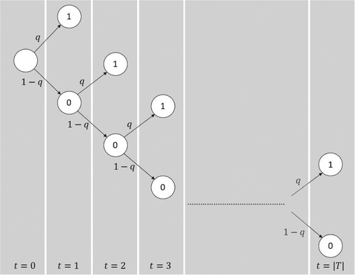
There are $|T|+1$ different scenarios. The disruption starts at time period $t$ in scenario $t$ except for the final scenario. To illustrate, the disruption starts at the $1^{st}$ time period in the $1^{st}$ scenario, it starts at the $2^{nd}$ time period in the $2^{nd}$ scenario, and so on. Note that there is no disruption in the final scenario. We can generate a matrix indicating whether there is a disruption in a given time period and scenario by combining this scenario tree and $TTR$ information. Figure 2 shows an example of this matrix (with $TTR=3$ time periods) as well as the corresponding scenario probabilities. Note that ‘1’ entries in the matrix indicate that the primary supplier is disrupted, whereas ‘0’ entries indicate that there is no disruption.

Figure 2. An example of the disruption matrix.

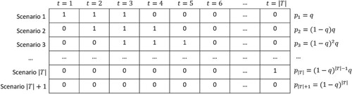
Note that $TTR$ and $q$ are deterministic inputs to our multistage stochastic programming model; however, we incorporate the ambiguity in these inputs by a decision support framework based on solving the proposed model for combinations of $TTR$ and the disruption probability during the life of the programme (derived from $q$ as shown in Figure 2). Our results in the next sections show that the optimal strategy is not overly sensitive to $TTR$ and the disruption probability.

3.8. Multistage stochastic programming model

Now that we have defined the decision variables and parameters, and described our scenario generation scheme, we can present our model: (1.1) $\begin{array}{rl}& \text{min}\sum _{l\in L_R}{f}_l^R{X}_l^R+\sum _{l\in L_B}{f}_l^B{X}_l^B+\sum _{l\in L_S}{f}_l^S{X}_l^S\\ & +\sum _{\omega \in \mathrm{\Omega }}{p}_{\omega }\sum _{l\in L_S\mathrm{\setminus }\left\{0\right\}}{f}_l^{S}X{P}_{l\omega }^S+c_P{I}_0^P+c_S{I}_0^S\end{array}$(1.1) (1.2) $\begin{array}{rl}& +\sum _{\omega \in \mathrm{\Omega }}{p}_{\omega }\left[\sum _{t\in T}{\left(1+i\right)}^{-t}\left(c_P\left(1+e_P{\delta }_{t\omega }\right)Y_{t\omega }^P\right)\right]\end{array}$(1.2) (1.3) $\begin{array}{rl}& +\sum _{\omega \in \mathrm{\Omega }}{p}_{\omega }\left[\sum _{t\in T}{\left(1+i\right)}^{-t}\left(c_S\left(Y_{t\omega }^S+e_{S}Y{P}_{t\omega }^S\right)\right)\right]\end{array}$(1.3) (1.4) $\begin{array}{rl}& +\sum _{\omega \in \mathrm{\Omega }}{p}_{\omega }\left[\sum _{t\in T}{\left(1+i\right)}^{-t}h{I}_{t\omega }\right]\end{array}$(1.4) (1.5) $\begin{array}{rl}& +\sum _{\omega \in \mathrm{\Omega }}{p}_{\omega }\left[\sum _{t\in T}{\left(1+i\right)}^{-t}b{L}_{t\omega })\right]\\ & -\sum _{\omega \in \mathrm{\Omega }}{p}_{\omega }\left[\sum _{t\in T\mathrm{\setminus }\left\{1\right\}}{\left(1+i\right)}^{-t}b{L}_{t-1,\omega })\right]\end{array}$(1.5) $s.t.$ (2) $\begin{array}{rl}& \sum _{l\in L_R}{X}_l^R=1\end{array}$(2) (3) $\begin{array}{rl}& \sum _{l\in L_B}{X}_l^B\le 1\end{array}$(3) (4) $\begin{array}{rl}& \sum _{l\in L_S}{X}_l^S\le 1\end{array}$(4) (5) $\begin{array}{rl}& Y_{t\omega }^P\le \left(1-{\rho }_{t\omega }\right)\left(1+a{\phi }_{t\omega }\right)\sum _{l\in L_R}{k}_l^R{X}_l^R+{\delta }_{t\omega }\sum _{l\in L_B}{k}_l^B{X}_l^B,\\ & \mathrm{\forall }t\in T,\omega \in \mathrm{\Omega }\end{array}$(5) (6) $\begin{array}{rl}& Y_{t\omega }^S\le \sum _{l\in L_S}{k}_l^S{X}_l^S+{\gamma }_{t\omega }Y{P}_{t\omega }^S,\mathrm{\forall }t\in T,\omega \in \mathrm{\Omega }\end{array}$(6) (7) $\begin{array}{rl}& Y{P}_{t\omega }^S\le \sum _{l\in L_S\mathrm{\setminus }\left\{0\right\}}{k}_l^{S}X{P}_{l\omega }^S,\mathrm{\forall }t\in T,\omega \in \mathrm{\Omega }\end{array}$(7) (8) $\begin{array}{rl}& \sum _{l\in L_S\mathrm{\setminus }\left\{0\right\}}X{P}_{l\omega }^S\le X_0^S,\mathrm{\forall }\omega \in \mathrm{\Omega }\end{array}$(8) (9) $\begin{array}{rl}& Y_{t\omega }^P+Y_{t\omega }^S+I_0^P+I_0^S-d=I_{t\omega }-L_{t\omega },\\ & t=1,\mathrm{\forall }\omega \in \mathrm{\Omega }\end{array}$(9) (10) $\begin{array}{rl}& Y_{t\omega }^P+Y_{t\omega }^S+I_{t-1,\omega }-L_{t-1,\omega }-d=I_{t\omega }-L_{t\omega },\\ & \mathrm{\forall }t\in T\mathrm{\setminus }\left\{1\right\},\omega \in \mathrm{\Omega }\end{array}$(10) (11) $\begin{array}{rl}& Y_{t\omega }^P\ge u^P\left(1-{\rho }_{t\omega }\right)\sum _{l\in L_R}{k}_l^R{X}_l^R,\mathrm{\forall }t\in T,\omega \in \mathrm{\Omega }\end{array}$(11) (12) $\begin{array}{rl}& Y_{t\omega }^S\ge u^S\sum _{l\in L_S}{k}_l^S{X}_l^S,\mathrm{\forall }t\in T,\omega \in \mathrm{\Omega }\end{array}$(12) (13) $\begin{array}{rl}& I_0^P\le m\sum _{l\in L_R}{k}_l^R{X}_l^R\end{array}$(13) (14) $\begin{array}{rl}& I_0^S\le m\sum _{l\in L_S}{k}_l^S{X}_l^S\end{array}$(14) (15) $\begin{array}{rl}& I_{t\omega }\le I_0^P+I_0^S,\mathrm{\forall }t\in T,\omega \in \mathrm{\Omega }\end{array}$(15) (16) $\begin{array}{rl}& Y_{t\omega }^P=Y_{t{\omega }^{\mathrm{\prime }}}^P,\mathrm{\forall }t\in T,\omega \in \mathrm{\Omega },\omega >\text{t},{\omega }^{\mathrm{\prime }}=|T|+1\end{array}$(16) (17) $\begin{array}{rl}& Y_{t\omega }^S=Y_{t{\omega }^{\mathrm{\prime }}}^S,\mathrm{\forall }t\in T,\omega \in \mathrm{\Omega },\omega >\text{t},{\omega }^{\mathrm{\prime }}=|T|+1\end{array}$(17) (18) $\begin{array}{rl}& X_l^R\in \left\{0,1\right\},\mathrm{\forall }l\in L_R\end{array}$(18) (19) $\begin{array}{rl}& X_l^B\in \left\{0,1\right\},\mathrm{\forall }l\in L_B\end{array}$(19) (20) $\begin{array}{rl}& X_l^S\in \left\{0,1\right\},\mathrm{\forall }l\in L_S\end{array}$(20) (21) $\begin{array}{rl}& X{P}_{l\omega }^S\in \left\{0,1\right\},\mathrm{\forall }l\in L_S\mathrm{\setminus }\left\{0\right\},\omega \in \mathrm{\Omega }\end{array}$(21) (22) $\begin{array}{rl}& I_0^P\ge 0\end{array}$(22) (23) $\begin{array}{rl}& I_0^S\ge 0\end{array}$(23) (24) $\begin{array}{rl}& Y_{t\omega }^P\ge 0\mathrm{\forall }t\in T,\omega \in \mathrm{\Omega }\end{array}$(24) (25) $\begin{array}{rl}& Y_{t\omega }^S\ge 0\mathrm{\forall }t\in T,\omega \in \mathrm{\Omega }\end{array}$(25) (26) $\begin{array}{rl}& Y{P}_{t\omega }^S\ge 0\mathrm{\forall }t\in T,\omega \in \mathrm{\Omega }\end{array}$(26) (27) $\begin{array}{rl}& I_{t\omega }\ge 0\mathrm{\forall }t\in T,\omega \in \mathrm{\Omega }\end{array}$(27) (28) $\begin{array}{rl}& L_{t\omega }\ge 0\mathrm{\forall }t\in T,\omega \in \mathrm{\Omega }\end{array}$(28)

The objective function minimises the expected total discounted cost including the fixed cost of reserving capacity from the suppliers, expected fixed cost of reserving capacity from the pre-qualified supplier, and cost of initial inventory (1.1), expected discounted primary supplier production cost (1.2), expected discounted secondary supplier production cost (1.3), expected discounted inventory holding cost (1.4), and expected discounted backordering cost (1.5). Note that the last term in the objective function ensures that the penalty incurred due to a backordered demand is recovered if the demand is satisfied subsequently. In this case, the cost of unmet demand is the interest lost on the backordering penalty.

Constraints (2), (3) and (4) are the capacity reservation constraints. Constraint (2) guarantees that a regular capacity level is reserved from the primary supplier. Constraint (3) ensures that at most one backup capacity level is chosen for this supplier. Similarly, constraint (4) makes sure that at most one capacity level is chosen for the secondary supplier.

Constraints (5) and (6) limit the amount of shipment by the capacity of the primary supplier and the secondary supplier, which depend on the functionality of the primary supplier’s regular capacity. The capacity of the primary supplier in time period $t\in T$ in scenario $\omega \in \mathrm{\Omega }$ can be represented by four different cases:

1. If there has not been a disruption (${\rho }_{t\omega }=0$ and ${\phi }_{t\omega }=0)$, the capacity is $\sum _{l\in L_R}{k}_l^R{X}_l^R$.

2. If there has been a disruption but the regular capacity is recovered (${\rho }_{t\omega }=0$ and ${\phi }_{t\omega }=1)$, the capacity is $\left(1+a\right)\sum _{l\in L_R}{k}_l^R{X}_l^R$.

3. If there is an ongoing disruption and $v$ time periods have passed after the disruption started to put the backup capacity in place $\left({\rho }_{t\omega }=1\text{ and }{\delta }_{t\omega }=1\right)$, the capacity is $\sum _{l\in L_B}{k}_l^B{X}_l^B$.

4. If there is an ongoing disruption and $v$ time periods have not passed after the disruption started to put the backup capacity in place $\left({\rho }_{t\omega }=1\text{ and }{\delta }_{t\omega }=0\right)$, the capacity is 0.

Likewise, the capacity of the secondary supplier at time period $t\in T$ in scenario $\omega \in \mathrm{\Omega }$ can be represented by two different cases:

1. If there is no disruption at the primary supplier or there is an ongoing disruption but $w$ time periods have not passed after the disruption started to place order from the pre-qualified supplier (${\gamma }_{t\omega }=0)$, the capacity is $\sum _{l\in L_S}{k}_l^S{X}_l^S.$

2. If there is an ongoing disruption and $w$ time periods have passed after the disruption started so that the pre-qualified supplier is ready for production (${\gamma }_{t\omega }=1)$, the capacity is $\sum _{l\in L_S}{k}_l^S{X}_l^S+Y{P}_{t\omega }^S$.

Constraints (7) ensure that the amount of shipment from the pre-qualified supplier does not exceed the capacity reserved from this supplier after the disruption. Constraints (8) does not allow the model to reserve any capacity after the disruption if the secondary supplier is not pre-qualified. Note that $X_0^S$ denotes the decision indicating whether the supplier is pre-qualified since level 0 is defined for the pre-qualification.

Constraints (9) and (10) are the inventory balance constraints. These constraints state that the sum of the total production at the current time period and the inventory at hand is used to satisfy the demand at the current time period (also any backordered demand from the previous time period). Excess parts after satisfying the demand are transferred to the next time period as inventory. Similarly, any demand not satisfied in this time period is transferred to the next time period as backordered demand.

Constraints (11) and (12) are utilisation constraints. Constraints (11) ensure that the capacity of the primary supplier is utilised above a determined threshold whenever the regular operations are not disrupted. Similarly, constraints (12) force the company to order from the secondary supplier to utilise a certain percentage of the reserved capacity. Note that when the company chooses level 0 (i.e. just pre-qualifying the secondary supplier instead of reserving any capacity beforehand), these constraints are reduced to (29) $Y_{t\omega }^S\ge 0,\mathrm{\forall }t\in T,\omega \in \mathrm{\Omega }$(29) saving the company to make any commitment to the secondary supplier.

Constraints (13) and (14) define the maximum inventory that can be built up before the launch using the capacity available at the primary supplier and secondary supplier, respectively. It is worth mentioning that this inventory is designated to be used mainly during the disruption periods. Therefore, constraints (15) avoid increasing the inventory level above the initial inventory level.

Constraints (16) and (17) are nonanticipativity constraints. In the multistage stochastic programming framework, nonanticipativity reflects the concept that the decision maker who cannot distinguish between scenarios progressing identically until time period $t$ makes the same decisions up to time period $t$. In our scenario tree, all scenarios are alike until the disruption starts. Therefore, ordering decisions should be the same across scenarios up to this point. Constraints (16) ensure that the order quantities placed to the primary supplier in scenario $\omega$ and in scenario $|T|+1$ are the same at time period $t$ if a disruption has not occurred $(\omega >t)$. Once again note that no disruption happens in scenario $|T|+1$ during the life of the programme. This is why this scenario can be used as a reference scenario.

Lastly, constraints (18) – (28) enforce binary and nonnegativity restrictions of the decision variables.

4. Decision support framework

The values of $TTR$ and $q$ should be identified to generate scenarios as presented in Section 3. Decision makers usually have a rough idea of the range of $TTR$, since they can pinpoint critical production processes and estimate the time needed for recovery if these processes are disrupted (Simchi-Levi et al. 2015; Kinra et al. 2020). (For a discussion on the uncertainty in $TTR$, please refer to Section A.4 of the online appendix.) However, it is very difficult to provide a point estimation of $TTR$. Furthermore, it is almost impossible to estimate the exact value of $q$, the probability that a disruption occurs in a time period, as it is typically a very small probability. Nevertheless, decision makers can provide their intuition on the probability that a disruption occurs anytime during the life of the programme; i.e. $1-p_{|T|+1}$ or $1-(1-q{)}^{|T|}$. We call this probability as the disruption probability in the rest of the paper. From this, we can compute $q$.

Our decision support framework is based on solving the proposed model for combinations of $TTR$ and the disruption probability. Our discussions with Ford reveal that the range of $TTR$ that they are interested in is between 2 and 20 weeks, and the range of the disruption probability is between 0% and 10%. Utilising this information, we generate the strategy graph which depicts the optimal strategies within the given range of $TTR$ and the disruption probability. A strategy graph for a hypothetical example is given in Figure 3. To create this graph, the model is solved for 100 different combinations of $TTR$ (2, 4 weeks, … , 20 weeks) and the disruption probability (1%, 2%, … , 10%). The optimal strategy is identified for each combination and depicted on the strategy graph. Note that this strategy graph is generated based on the range of $TTR$ and the disruption probability on Ford’s radar; however, it is quite straightforward to use this framework for different ranges that other companies might be interested in.

Figure 3. An example strategy graph.

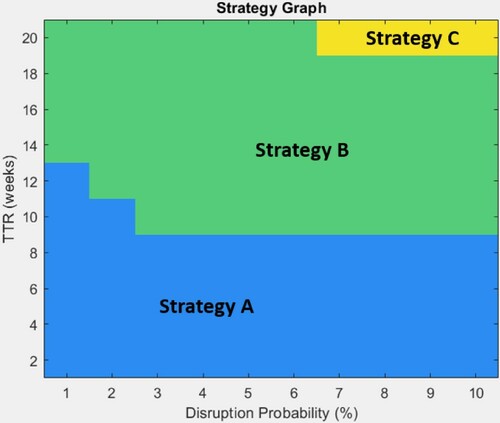
Figure 3 shows that there are three strategies which are optimal in different parts of the graph. The advantage of using this strategy graph is that decision makers do not need to estimate $TTR$ and the disruption probability precisely. For example, Figure 3 suggests that regardless of the estimated disruption probability, Strategy A is the optimal strategy if TTR is less than or equal to eight weeks. Moreover, strategy B is the optimal strategy if $TTR$ is more than 8 weeks and the disruption probability is between 3% and 6%. If decision makers agree that $TTR$ is 20 weeks but they cannot agree on whether the disruption probability is more than 6%, they can compare the expected total cost when Strategy B or Strategy C is implemented. Our results from the case study at Ford in the next section indicate that the difference between the expected cost of implementing these neighbouring strategies can be insignificant. Therefore, the regret in using the non-optimal strategy when the probability is not estimated precisely tends to be small.

5. Case study

Following a major supply disruption during 2018, Ford began considering the use of mitigation strategies to protect against supply disruption risks for critical parts. The feasible strategies under discussion are given in Table 2. Each strategy is described by a triplet giving the regular capacity at the primary supplier, backup capacity at the primary supplier, and capacity at the secondary supplier. Note that $x\mathrm{\%}$ capacity represents the capacity sufficient to satisfy $x\mathrm{\%}$ of the demand. Along with this triplet, the strategy name also indicates whether backup inventory is allowed or not.

Table 2. Feasible strategies under discussion.

Mitigation Strategy	Strategy Name	Regular Capacity at the Primary Supplier	Backup Capacity at the Primary Supplier	Capacity at the Secondary Supplier	Backup Inventory
No mitigation	No Mitigation:(100%,0%,0%) no inventory	100%	0%	0%	No
Backup inventory	Backup Inventory:(100%,0%,0%) with inventory	100%	0%	0%	Yes
Dual sourcing	Dual Sourcing I:(50%,0%,50%) no inventory	50%	0%	50%	No
	Dual Sourcing II:(100%,0%,100%) no inventory	100%	0%	100%	No
	Dual Sourcing III:(100%,0%,pq) no inventory	100%	0%	Pre-qualified	No
Backup capacity	Backup Capacity I:(100%,50%,0%) no inventory	100%	50%	0%	No
	Backup Capacity II:(100%,100%,0%) no inventory	100%	100%	0%	No

Note that there are more strategies available other than the ones listed in Table 2. For example, the company can integrate backup inventory with the dual sourcing strategy in which the capacity is reserved from the primary supplier to satisfy 50% of the demand and the capacity is reserved from the secondary supplier to satisfy 50% of the demand; i.e. integrate Backup Inventory with Dual Sourcing I. In this way, the company can satisfy half of the demand from the secondary supplier and the other half from the backup inventory whenever the primary supplier is disrupted. However, before allowing hybrid strategies, we consider only these core strategies to perform a comparative analysis to gain insights into their upsides and downsides.

In this section, we conduct our analyses for the vehicle part whose production was disrupted due to an extreme event at the supplier’s plant. We obtained the unit cost per part and the tooling cost information from the market test performed by the purchasing experts. Unfortunately, we can share neither the cost figures nor the names of the potential suppliers due to confidentiality concerns. We also cannot provide the demand of the vehicle and the profit margin per vehicle (corresponding to the backordering penalty). We present the values of other parameters used in this case study in Table 3.

Table 3. Values of the uncensored parameters used in the case study.

$h:$ inventory holding cost per unit per time period	$h=\mathrm{\$}0.02$
$m$: number of time periods available to build up the initial inventory	$m=8$ weeks
$v$: number of time periods needed for the backup capacity to be in place	$v=2$ weeks
$w$: number of time periods needed for the pre-qualified supplier’s capacity to be in place	$w=6$ weeks
$e_P:$ increase in unit cost of parts supplied from the primary supplier when backup capacity is used	$e_P=0.50$
$e_S:$ increase in unit cost of parts supplied from the pre-qualified supplier	$e_S=1.00$
$u^P$: minimum utilisation rate of the primary supplier	$u^P=50\mathrm{\%}$
$u^S$: minimum utilisation rate of the secondary supplier	$u^S=50\mathrm{\%}$
$a$: allowance in the capacity of the primary supplier	$a=15\mathrm{\%}$
$i:$ effective interest rate for time period	$i=0.0425\mathrm{\%}$

Note that we use weeks to represent time periods in the planning horizon, and we consider that the planning horizon consists of $3\text{years}\times 46\frac{\text{weeks}}{\text{year}}=138\text{weeks}$.

To generate the strategy graph for this case study, we solved the MIP equivalent of the multistage stochastic programming models corresponding to each combination of $TTR$ and the disruption probability. We used IBM ILOG Cplex 12.9 operating on an Intel(R) Core(TM) i7-8565U CPU 1.80 GHz, 16 GB RAM machine with Windows 10. Note that each MIP model has 285 binary decision variables and 95,912 nonnegative decision variables. Cplex solved each one of these models to optimality with an average CPU time of 302.4 s.

Before presenting the strategy graph for this case study, we investigate the effect of implementing the strategies given in Table 2 on the expected total cost. We compare the expected total cost of these strategies with the optimal expected total cost if there is no disruption risk. Note that No Mitigation is the optimal strategy when there is no disruption risk.

Similar to the strategy graph, we generate heat maps to visualise the relative expected total cost of a strategy as a function of $TTR$ and the disruption probability. We define the relative expected total cost of a strategy as the ratio of the expected total cost of this strategy to the optimal expected total cost if there is no disruption risk. Note that we add the leftmost column in our heat maps to show the relative expected total cost when the disruption probability is 0%.

Next, we discuss the effect of implementing mitigation strategies using these heat maps. We also support our claims with the plots illustrating the change in the cost components with respect to $TTR$ (fixing the disruption probability to 10%). We group the cost components into five: capacity cost and initial inventory cost, expected production cost (primary supplier), expected production cost (secondary supplier), expected inventory holding cost, and expected backordering cost. These cost components correspond to the objective function components presented in Section 3. Due to confidentiality concerns, we cannot provide the cost values on the plots. Similar to the heat maps, the cost values on these plots are scaled based on the optimal expected total cost if there is no disruption risk.

5.1. Mitigation through backup inventory

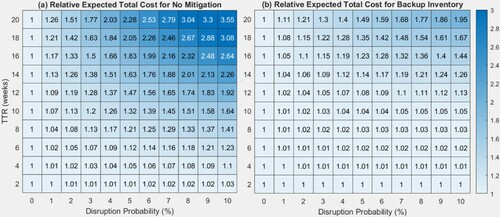
The heat map depicted in Figure 4a shows the relative expected total cost for No Mitigation in Table 2 with respect to $TTR$ and the disruption probability. The heat map indicates that the expected total cost of relying on this strategy goes up significantly as $TTR$ and the disruption probability increase. On the other hand, Figure 4b, which represents the heat map of the relative expected total cost for Backup Inventory in Table 2, reveals that solely using inventory helps to reduce the expected total cost to a great extent. We observe that inventory mitigation is especially effective when $TTR$ is less than or equal to eight weeks available in the pre-production stage to build up inventory.

Figure 4. Relative expected total cost for No Mitigation and Backup Inventory.

As we mention above, we also generate the plots of cost components with respect to $TTR$ when we fix the disruption probability to 10%. Figure 5a and Figure 5b show the change in the cost components with respect to $TTR$ for the No Mitigation and Backup Inventory strategies, respectively. We add the leftmost bars to represent the relative costs in case there is no disruption risk ($TTR=0$). Note that these leftmost bars in both figures are identical since the Backup Inventory strategy also holds zero inventory when there is no disruption risk. These bars indicate that the expected production cost constitutes a large portion of the expected total cost compared to the capacity cost. In fact, the capacity cost is approximately 4% of the expected total cost when there is no disruption risk. Figure 5a shows that the level of the capacity cost does not change for No Mitigation as $TTR$ increases; however, Figure 5b indicates a slight increase in this cost component as we allow for the creation of the backup inventory. Note that this increase is limited as the level of inventory cannot exceed eight weeks of inventory. When the inventory level is at its maximum allowed level, the capacity and initial inventory cost is approximately 10% of the reference cost, which is still a small portion of the overall cost. In addition to the cost of building up initial inventory, there is also the expected inventory holding cost associated with carrying inventory from one week to the next week. However, we observe from Figure 5b that this cost component is not significant compared to the other cost components.

Figure 5. Relative cost components w.r.t. TTR for No Mitigation and Backup Inventory (Disruption Probability = 10%).

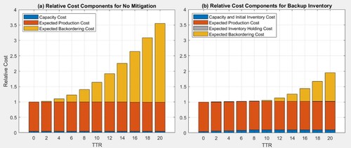
A significant cost component entering the picture as we increase $TTR$ is the expected backordering cost. Figure 5a suggests that the expected backordering cost increases dramatically for No Mitigation as $TTR$ increases. According to Figure 5b, Backup Inventory keeps the expected backordering cost under control for smaller $TTR$ values. However, we observe the steep increase in the expected backordering cost for Backup Inventory as well if the initial inventory is not sufficient to satisfy the demand during the disruption.

5.2. Mitigation through dual sourcing

Figure 6 presents the relative expected total costs for the three dual sourcing strategies in Table 2. We observe from Figure 6a that Dual Sourcing I is not an effective mitigation strategy. This strategy offers improvement in the expected total cost over No Mitigation only for high values of $TTR$ and the disruption probability. Although half of the demand can be satisfied from the secondary supplier, Dual Sourcing I does not provide an alternative to source parts ordered from the primary supplier when this supplier is disrupted. On the other hand, Dual Sourcing II allows the secondary supplier to pick up the orders from the primary supplier during the disruption periods. As we can see from Figure 6b, this strategy is quite robust for all combinations of $TTR$ and the disruption probability. Note that when the disruption probability is 0%, the expected total costs of Dual Sourcing I and Dual Sourcing II increase by 23% and 29% compared to the expected total cost of No Mitigation, respectively. The main reason for the increase in the expected total cost is the expected cost of production at the secondary supplier. Both Dual Sourcing I and Dual Sourcing II commit to the expensive secondary supplier to order parts during the life of the programme; however, Dual Sourcing III uses this supplier only during the disruption periods. Figure 6c shows that Dual Sourcing III is a more advantageous strategy in a broader range among the three dual sourcing strategies.

Figure 6. Relative expected total cost for Dual Sourcing I, Dual Sourcing II, and Dual Sourcing III.

Next, we examine the plots of cost components with respect to $TTR$ generated for Dual Sourcing I, Dual Sourcing II, and Dual Sourcing III. Like Figure 5 above, we fix the disruption probability to 10% for this analysis. Note that the vertical scales of Figure 7 differ from those of Figure 5. We observe from Figure 7b that Dual Sourcing II requires a higher level of initial investment as it installs sufficient capacity to produce 200% of the demand when there is no disruption. Figure 7a and Figure 7c suggest that Dual Sourcing I and Dual Sourcing III have similar capacity costs. There is only a small increase in the capacity cost for Dual Sourcing III due to the initial investment to pre-qualify the secondary supplier. Furthermore, the increase in the expected cost due to the capacity installed after the disruption is insignificant compared to this initial investment needed for the pre-qualification.

Figure 7. Relative cost components w.r.t. TTR for Dual Sourcing I, Dual Sourcing II, and Dual Sourcing III (Disruption Probability = 10%).

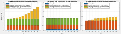
Figure 7a and Figure 7b show that the expected production costs at the primary supplier in Dual Sourcing I and Dual Sourcing II are almost half of the costs in No Mitigation and Dual Sourcing III. Note that Dual Sourcing I and Dual Sourcing II require ordering from the secondary supplier regularly. Therefore, these strategies split the orders between both suppliers.

Dual Sourcing II is the most effective strategy in dealing with the unmet demand. As we observe from Figure 7b, the expected backordering cost is almost zero under this strategy since demand can be completely satisfied from the secondary supplier when the disruption occurs. Figure 7a shows that Dual Sourcing I cannot cope with the increasing number of backordered demands as the secondary supplier can produce at most 50% of the demand when the primary supplier is disrupted. Finally, we can observe from Figure 7c that Dual Sourcing III results in backordering costs during six weeks needed for the pre-qualified supplier to start production.

5.3. Mitigating through backup capacity at the primary supplier

Figure 8 shows the relative expected total costs for Backup Capacity I and Backup Capacity II in Table 2. These figures illustrate that having an adequate level of the backup capacity at the primary supplier is effective in reducing the expected total cost. When the disruption probability is 0%, the expected total costs of Backup Capacity I and Backup Capacity II increase by only 2% and 4% respectively compared to the expected total cost of No Mitigation. In return, the savings in the expected total cost are very significant when the disruption probability is greater than 0%.

Figure 8. Relative expected total cost for Backup Capacity I and Backup Capacity II.

Next, we also present the plots of cost components generated for Backup Capacity I and Backup Capacity II when the disruption probability is 10%. Compared to No Mitigation, the capacity cost increases by 50% and by 100% under Backup Capacity I and Backup Capacity II, respectively. However, Figure 9a and Figure 9b indicate that the increase in the capacity cost when reserving backup capacity is insignificant since the capacity cost itself has a small share in the expected total cost, as discussed above.

Figure 9. Relative cost components w.r.t. TTR for Backup Capacity I and Backup Capacity II (Disruption Probability = 10%).

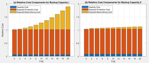
Figure 9a shows that Backup Capacity I cannot handle the increase in the backordered demand as the backup capacity is only able to produce 50% of the demand during the disruption periods. Backup Capacity II has sufficient capacity to produce 100% of the demand during the disruption periods; however, we still observe a slight increase in the expected backordering cost in Figure 9b since it takes two weeks to restore the backup capacity at the primary supplier. Note that the demand backordered during these weeks cannot be met until the regular capacity is back with an increase in the production rate.

5.4. Strategy graph

As discussed earlier, the feasible strategies are not limited to these seven strategies analysed above. In fact, building up backup inventory can be complementary for strategies like Dual Sourcing I and Backup Capacity I. In Figure 10, we present the strategy graph generated by allowing hybrid strategies. We also provide the inventory graph showing the initial inventory levels corresponding to the optimal mitigation strategy.

Figure 10. Strategy graph and inventory graph.

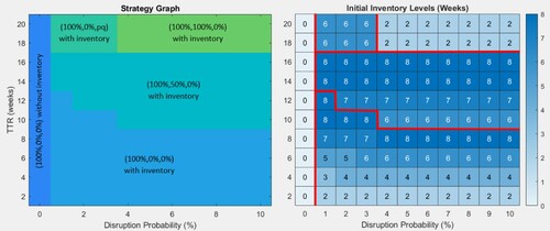
Figure 10 suggests that there are five optimal strategies within the range determined for $TTR$ and the disruption probability. The strategy of solely reserving 100% capacity from the primary supplier is only optimal when the disruption probability is 0%. We observe that the strategy of reserving 100% capacity from the primary supplier and building up backup inventory is the optimal strategy when there is disruption risk and $TTR$ is less than or equal to eight weeks. This means that when $TTR$ is expected to be smaller than the time available before the launch, it is still optimal to use single sourcing without any additional backup capacity. Inventory mitigation is an effective strategy in this case. When we examine the inventory graph, we see that the inventory level is exactly the level required to satisfy the demand during the disruption (up to a maximum of eight weeks of inventory) if the disruption probability is more than 3%. When the disruption probability is low, the inventory level can be slightly less than the exact amount required during the disruption.

If $TTR$ is more than eight weeks but less than or equal to sixteen weeks, the dominant strategy is reserving 50% backup capacity from the primary supplier in addition to 100% regular capacity. In this case, half of the demand is satisfied through the backup capacity and the other half is satisfied through the initial inventory during the disruption. Therefore, the inventory level under this strategy tends to be approximately half of the level needed to satisfy the demand during $TTR$ weeks. The reason that the inventory level is slightly more than this level is the two weeks of preparation time for the backup capacity.

When $TTR$ is more than sixteen weeks, it is optimal to reserve 100% regular and 100% backup capacity from the primary supplier if the disruption probability is more than 3%. In this case, the optimal inventory level is only for two weeks. These two weeks of inventory are held to satisfy the demand during the time needed to install the backup capacity at the primary supplier. If the disruption probability is less than or equal to 3% (but more than 0%), the optimal strategy is to reserve 100% capacity from the primary supplier and pre-qualify the secondary supplier. Under this strategy, it is optimal to have six weeks of inventory to satisfy the demand during the time needed to prepare the secondary supplier for production.

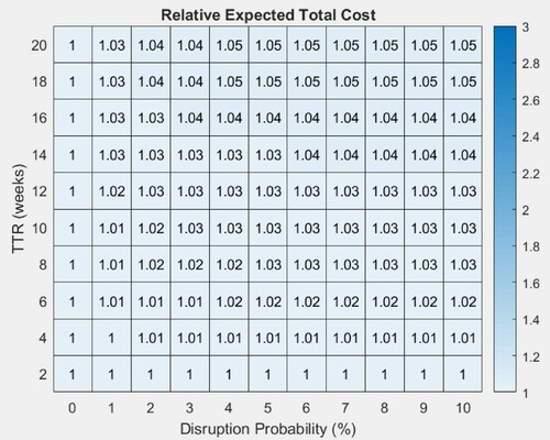
Figure 11 shows the relative expected total cost of the strategies given in the strategy graph. Recall that the relative expected total cost is computed based on the optimal expected total cost when there is no disruption. In other words, the reference point is the expected total cost of No Mitigation when the disruption probability is 0%. We observe from Figure 11 that even when $TTR$ is 20 weeks and the disruption probability is 10%, the expected total cost increases by 5% compared to the optimal expected total cost if there was no disruption risk. When we check Figure 4 again, we see that the expected total cost of No Mitigation under this most extreme case is 3.55 times the expected total cost of No Mitigation under no disruption risk. This means that the expected total cost can increase drastically if the sourcing strategy is chosen without accounting for the disruption risk. However, it is possible to mitigate the increase in the expected total cost by using an adequate strategy based on the risk profile defined by $TTR$ and the disruption probability.

Figure 11. Relative expected total cost for the strategy grap.

We also analyse the relative expected total cost of all five strategies shown on the strategy graph. We have already presented the heat maps for the (100%, 0%, 0%) strategy without inventory (No Mitigation in Table 2) and the (100%, 0%, 0%) strategy with inventory (Backup Inventory in Table 2) in Figure 4. Figure 12 illustrates the heat maps of the relative expected total cost for the (100%, 50%, 0%) strategy with inventory, the (100%, 100%, 0%) strategy with inventory, and the (100%, 0%, pq) strategy with inventory.

Figure 12. Relative expected total cost for the optimal strategies on the strategy graph.

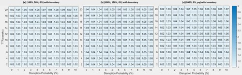
As we can observe from Figure 12, these hybrid strategies are quite robust over all values of $TTR$ and the disruption probability. Moreover, we observe that there are no significant differences between the expected total costs of neighbouring strategies on the borders defining optimal strategies. For example, it is optimal to pre-qualify the secondary supplier or reserve 100% backup capacity from the primary supplier when $TTR$ is more than 16 weeks. The disruption probability determines which of these two mitigation strategies is optimal. However, even if the disruption probability could not be estimated precisely, the regret of using the non-optimal strategy would be small. To illustrate, suppose that the true disruption probability is 3%, but the decision makers overestimate this probability as 6%. Therefore, the optimal strategy is identified as reserving 100% backup capacity from the primary supplier instead of pre-qualifying the secondary supplier. In this case, the expected total cost would only increase by 0.2% when $TTR$ is 20 weeks. In the opposite case, where the true disruption probability is 6% but is underestimated as 3%, the expected total cost would increase by 0.7%. All in all, the regret of using the non-optimal strategy due to an imprecise estimation is at most 1.3% of the optimal expected total cost, when the probability estimations are within the range of 1% to 10%. However, the increase in the expected total cost can be drastic when the disruption risk is completely ignored (i.e. the disruption probability is assumed to be 0%, but the disruption risk does exist). For example, when $TTR$ is 20 weeks, the expected total cost would increase to 1.7 and 2.4 times the optimal expected total cost when the true disruption probability is 3% and 6%, respectively.

This section points out important results for the case study in question. In this case study, the optimal mitigation strategy is to use inventory mitigation when $TTR$ is less than the time available to build up the backup inventory. When $TTR$ is longer, it is optimal to use the backup capacity at the primary supplier or to pre-qualify the secondary supplier depending on the estimated value of $TTR$ and the disruption probability. Note that our findings are in line with Tomlin (2006). In this seminal paper, Tomlin (2006) also points out that in an environment of rare but long disruptions, sourcing mitigation becomes more attractive over inventory mitigation since the latter requires carrying an excessive level of inventory for extended periods without any disruption.

A noteworthy observation in this case study is that the inventory holding costs and the capacity costs are relatively low compared to the production costs and the backordering costs. For sensitivity analyses, we investigated how our results would change for problem environments in which the cost of holding inventory and the cost of adding more capacity are higher. We also investigated the case in which decision makers’ $TTR$ estimation is not exact; i.e. $TTR$ uncertainty exists. Finally, we analysed the sensitivity of the strategy graph to certain parameters. We present our sensitivity analyses results in the online appendix (Sections A.2 – A.5).

6. Conclusions

In this study, we develop a decision support framework with Ford to choose the best mitigation strategy against supply disruptions when sourcing a critical part. The building block of the framework is a multistage stochastic programming model. This model determines the mitigation strategy to use before the launch of a new programme when the disruption uncertainty has not been resolved. By solving this model for possible $TTR$ and disruption probability combinations, we generate the strategy graph to illustrate the optimal strategies. The strategy graph aids decision makers to choose the best mitigation strategy based on their intuition on the values of $TTR$ and the disruption probability.

We discuss our results using a case study based on a business example at Ford. This case study demonstrates that relying solely on the regular capacity of the primary supplier, which is optimal when there is no disruption risk, can increase the expected total cost substantially when the disruption probability is not 0%. The impact of ignoring the disruption risk on the expected total cost can be large especially for higher values of $TTR$. However, a proper mitigation strategy can alleviate the increase in the expected total cost even for the extreme values of $TTR$ and the disruption probability. Our results show that holding backup inventory is an effective strategy for smaller values of $TTR$ when the backup inventory level is sufficient to satisfy demand during the disruption. For larger values of $TTR$, it is more appealing to integrate inventory mitigation with reserving backup capacity from the primary supplier or with pre-qualifying the secondary supplier. Our results point out the robustness of these hybrid strategies over all possible combinations of $TTR$ and the disruption probability.

There are several interesting future directions emerging from this research. Our attention in this paper is on the supply disruption risk; however, it is necessary to incorporate other supply chain risks and their interdependencies when making strategic sourcing decisions (Aqlan and Lam 2015). Analysing such correlations within the problem environment presented in this study is a notable research direction. Another prominent extension is to account for multiple suppliers subject to multiple disruptions in the supply chain network design context, by also considering the disruption propagation and the so-called ripple effect (Liberatore, Scaparra, and Daskin 2012; Dolgui, Ivanov, and Sokolov 2018). This has become an urgent topic in the COVID-19 era as the supply chains have been experiencing unprecedented supply disruptions since the beginning of the outbreak. Finally, it is worthy of considering different objective functions such as maximising profit and minimising conditional value-at-risk of cost or multiple objectives addressing the tradeoff between cost and reliability.

Acknowledgments

This work is supported by a grant from the Ford Motor Company, project grant number N025042. We are thankful to Colleen Montgomery, Scott Moore, Christopher Recktenwald, Paul Prestel from Ford Purchasing and Varsha Venkatesh from Ford Global Data, Insight and Analytics for their valuable contribution. Also, we would like to extend our thanks to the associate editor and anonymous reviewers for their insightful comments and constructive suggestions to improve the manuscript.

Disclosure statement

No potential conflict of interest was reported by the author(s).

Additional information

Funding

This work was supported by Ford Motor Company: [Grant Number N025042].

Notes on contributors

Ece Sanci

Ece Sanci is a Lecturer (Assistant Professor) in the Information, Decisions & Operations division of the School of Management at the University of Bath. She received her Ph.D. in Industrial and Operations Engineering in 2019 from the University of Michigan, Ann Arbor. She received her B.S. and M.S. in Industrial Engineering in 2013 and 2015 from the Middle East Technical University (METU) in Ankara. Her research focuses on decision making under uncertainty with applications in disaster relief management and supply chain risk management.

Mark S. Daskin

Mark S. Daskin is the Clyde W. Johnson Collegiate Professor in the Industrial and Operations Engineering Department of the University of Michigan at Ann Arbor. He served as the chair of the department for almost nine years beginning in 2010. Prior to joining the Michigan faculty, he was on the faculty at Northwestern University, where he also served as the chair of the Industrial Engineering and Management Sciences Department for six years. He is a former editor-in-chief of both Transportation Science and IIE Transactions. He is the author of two books: Service Science, and Network and Discrete Location: Models, Algorithms, and Applications.

Young-Chae Hong

Young-Chae Hong is a research scientist at Ford Motor Company. He received his Ph.D. degree in Industrial and Operations Engineering from the University of Michigan at Ann Arbor in 2017. His research interests are in large-scale optimization problems and machine learning algorithms to improve computational time. He worked as a research assistant at the Center for Healthcare Engineering and Patient Safety (CHEPS) for healthcare scheduling problems. He is currently working on three major research topics: supply chain analytics, routing with bin packing problem, and quantum algorithm.

Steve Roesch

Steve Roesch is a data scientist at Chewy. He worked as an analytics scientist at Ford Motor Company between 2017 and 2021. He received his Ph.D. degree in Industrial and Systems Engineering in 2017 from Virginia Polytechnic Institute and State University.

Don Zhang

Don (Xiaodong) Zhang received his Ph.D. and M.S. degrees in Materials Science and Engineering from Carnegie Mellon University, Pittsburgh, PA, USA. Currently, he is a Technical Expert and data scientist supervisor in the Global Data Insight and Analytics at Ford Motor Company.

References

- Aldrighetti, R., D. Battini, D. Ivanov, and I. Zennaro. 2021. “Costs of Resilience and Disruptions in Supply Chain Network Design Models: A Review and Future Research Directions.” International Journal of Production Economics 235: 108103.
- Aqlan, F., and S. S. Lam. 2015. “Supply Chain Risk Modelling and Mitigation.” International Journal of Production Research 53 (18): 5640–5656.
- Baghalian, A., S. Rezapour, and R. Z. Farahani. 2013. “Robust Supply Chain Network Design with Service Level Against Disruptions and Demand Uncertainties: A Real-Life Case.” European Journal of Operational Research 227: 199–215.
- Berger, P. D., A. Gerstenfeld, and A. Z. Zeng. 2004. “How Many Suppliers are Best? A Decision-Analysis Approach.” Omega 32: 9–15.
- Berger, P. D., and A. Z. Zeng. 2006. “Single Versus Multiple Sourcing in the Presence of Risks.” Journal of the Operational Research Society 57 (3): 250–261.
- Blome, C., and M. Henke. 2009. “Single Versus Multiple Sourcing: A Supply Risk Management Perspective.” In Supply Chain Risk: A Handbook of Assessment, Management, and Performance, edited by G. A. Zsidisin, and B. Richie, 125–135. New York, US: Springer.
- Chen, J., X. Zhao, and Y. Zhou. 2012. “A Periodic-Review Inventory System with a Capacitated Backup Supplier for Mitigating Supply Disruptions.” European Journal of Operational Research 219: 312–323.
- Chopra, S., G. Reinhardt, and U. Mohan. 2007. “The Importance of Decoupling Recurrent and Disruption Risks in a Supply Chain.” Naval Research Logistics 54 (5): 544–555.
- Chopra, S., and M. Sodhi. 2004. “Managing Risk to Avoid Supply Chain Breakdown.” MIT Sloan Management Review 46: 53–61.
- Dada, M., N. C. Petruzzi, and L. B. Schwarz. 2007. “A Newsvendor’s Procurement Problem When Suppliers are Unreliable.” Manufacturing & Service Operations Management 9 (1): 9–32.
- Dolgui, A., D. Ivanov, and B. Sokolov. 2018. “Ripple Effect in the Supply Chain: an Analysis and Recent Literature.” International Journal of Production Research 56 (1-2): 414–430.
- Federgruen, A., and N. Yang. 2009. “Optimal Supply Diversification Under General Supply Risks.” Operations Research 57 (6): 1451–1468.
- Gupta, V., B. He, and S. P. Sethi. 2015. “Contingent Sourcing Under Supply Disruption and Competition.” International Journal of Production Research 53 (10): 3006–3027.
- Hosseini, S., N. Morshedlou, D. Ivanov, M. D. Sarder, K. Barker, and A. Al Khaled. 2019. “Resilient Supplier Selection and Optimal Order Allocation Under Disruption Risks.” International Journal of Production Economics 213: 124–137.
- Hu, B., and D. Kostamis. 2015. “Managing Supply Disruptions When Sourcing from Reliable and Unreliable Suppliers.” POM 24 (5): 808–820.
- Ivanov, D., and A. Dolgui. 2019. “Low-Certainty-Need (LCN) Supply Chains: A New Perspective in Managing Disruption Risks and Resilience.” International Journal of Production Research 57 (15): 5119–5136.
- Ivanov, D., A. Dolgui, B. Sokolov, and M. Ivanova. 2017. “Literature Review on Disruption Recovery in the Supply Chain.” International Journal of Production Research 55 (20): 6158–6174.
- Jahani, H., B. Abbasi, Z. Hosseinifard, M. Fadaki, and J. P. Minas. 2020. “Disruption Risk Management in Service-Level Agreements.” International Journal of Production Research, doi:10.1080/00207543.2020.1748248.
- Kim, M., and C. Jim. 2011, March 14. “Global Supply Chain Rattled by Japan Quake, Tsunami.” https://www.reuters.com/article/japan-quake-supplychain/update-3-global-supply-chain-rattled-by-japan-quake-tsunami-idUSL3E7EE05V20110314.
- Kinra, A., D. Ivanov, A. Das, and A. Dolgui. 2020. “Ripple Effect Quantification by Supplier Risk Exposure Assessment.” International Journal of Production Research 58: 5559–5578.
- Kleindorfer, P. R., and G. H. Saad. 2005. “Managing Disruption Risks in Supply Chains.” POM 14: 53–68.
- Konrad, W. 2018, February 12. “Why So many Medicines are in Short Supply Months after Hurricane Maria.” https://www.cbsnews.com/news/why-so-many-medicines-arel-in-short-supply-after-hurricane-maria/.
- Liberatore, F., M. P. Scaparra, and M. S. Daskin. 2012. “Hedging Against Disruptions with Ripple Effects in Location Analysis.” Omega 40: 21–30.
- Lücker, F., S. Chopra, and R. W. Seifert. 2021. “Mitigating Product Shortage Due to Disruptions in Multi-Stage Supply Chains.” POM 30: 941–964.
- Mak, H., and Z. M. Shen. 2012. “Risk Diversification and Risk Pooling in Supply Chain Design.” IIE Transactions 44 (8): 603–621.
- Masih-Tehrani, B., S. H. Xu, S. Kumara, and H. Li. 2011. “A Single-Period Analysis of a Two-Echelon Inventory System with Dependent Supply Uncertainty.” Transportation Research Part B 45: 1128–1151.
- Meena, P. L., S. P. Sarmah, and A. Sarkar. 2011. “Sourcing Decisions Under Risks of Catastrophic Event Disruptions.” Transportation Research Part E 47: 1058–1074.
- Mehra, S., and R. A. Inman. 1992. “Determining the Critical Elements of Just-in-Time Implementation.” Decision Sciences 23: 160–174.
- Mohammaddust, F., S. Rezapour, R. Z. Farahani, M. Mofidfar, and A. Hill. 2017. “Developing Lean and Responsive Supply Chains: A Robust Model for Alternative Risk Mitigation Strategies in Supply Chain Designs.” International Journal of Production Economics 183: 632–653.
- Namdar, J., X. Li, R. Sawhney, and N. Pradhan. 2018. “Supply Chain Resilience for Single and Multiple Sourcing in the Presence of Disruption Risks.” International Journal of Production Research 56 (6): 2339–2360.
- Nishiguchi, T., and A. Beaudet. 1998. “Case Study: The Toyota Group and the Aisin Fire.” Sloan Management Rev 40 (1): 49–59.
- Norrman, A., and U. Jansson. 2004. “Ericsson’s Proactive Supply Chain Risk Management Approach After a Serious sub-Supplier Accident.” International Journal of Physical Distribution & Logistics Management 34 (5): 434–456.
- Paul, S. K., R. Sarker, and D. Essam. 2017. “A Quantitative Model for Disruption Mitigation in a Supply Chain.” European Journal of Operational Research 257: 881–895.
- Peng, P., L. V. Snyder, A. Lim, and Z. Liu. 2011. “Reliable Logistics Networks Design with Facility Disruptions.” Transportation Research Part B 45: 1190–1211.
- Qi, L. 2013. “A Continuous-Review Inventory Model with Random Disruptions at the Primary Supplier.” European Journal of Operational Research 225: 59–74.
- Qi, L., and Z. M. Shen. 2007. “A Supply Chain Design Model with Unreliable Supply.” Naval Research Logistics 54 (8): 829–844.
- Qi, L., Z. M. Shen, and L. V. Snyder. 2010. “The Effect of Supply Disruptions on Supply Chain Design Decisions.” Transportation Science 44 (2): 274–289.
- Ruiz-Torres, A. J., and F. Mahmoodi. 2007. “The Optimal Number of Suppliers Considering the Costs of Individual Supplier Failures.” Omega 35: 104–115.
- Salehi Sadghiani, N., S. A. Torabi, and N. Sahebjamnia. 2015. “Retail Supply Chain Network Design Under Operational and Disruption Risks.” Transportation Research Part E 75: 95–114.
- Sarkar, A., and P. K. J. Mohapatra. 2009. “Determining the Optimal Size of Supply Base with the Consideration of Risks of Supply Disruptions.” International Journal of Production Economics 119: 122–135.
- Sawik, T. 2011. “Selection of Supply Portfolio Under Disruption Risks.” Omega 39: 194–208.
- Sawik, T. 2017. “A Portfolio Approach to Supply Chain Disruption Management.” International Journal of Production Research 55 (7): 1970–1991.
- Sawik, T. 2019. “Two-period vs. Multi-Period Model for Supply Chain Disruption Management.” International Journal of Production Research 57 (14): 4502–4518.
- Schmitt, A. J. 2011. “Strategies for Customer Service Level Protection Under Multi-Echelon Supply Chain Disruption Risk.” Transportation Research Part B 45: 1266–1283.
- Schmitt, A. J., and L. V. Snyder. 2012. “Infinite-horizon Models for Inventory Control Under Yield Uncertainty and Disruptions.” Computers & Operations Research 39: 850–862.
- Simchi-Levi, D., W. Schmidt, Y. Wei, P. Y. Zhang, K. Combs, Y. Ge, O. Gusikhin, M. Sanders, and D. Zhang. 2015. “Identifying Risks and Mitigating Disruptions in the Automotive Supply Chain.” Interfaces 45 (5): 375–390.
- Snoeck, A., M. Udenio, and J. C. Fransoo. 2019. “A Stochastic Program to Evaluate Disruption Mitigation Investments in the Supply Chain.” European Journal of Operational Research 274: 516–530.
- Snyder, L. V., Z. Atan, P. Peng, Y. Rong, A. J. Schmitt, and B. Sinsoysal. 2016. “OR/MS Models for Supply Chain Disruptions: a Review.” IIE Transactions 48 (2): 89–109.
- Snyder, L. V., and M. S. Daskin. 2005. “Reliability Models for Facility Location: The Expected Failure Cost Case.” Transportation Science 39 (3): 400–416.
- Sugimori, Y., K. Kusunoki, F. Cho, and S. Uchikawa. 1977. “Toyota Production System and Kanban System Materialization of Just-in-Time and Respect-for-Human System.” International Journal of Production Research 15: 553–564.
- Tang, C. S. 2006. “Perspectives in Supply Chain Risk Management.” International Journal of Production Economics 103: 451–488.
- Tomlin, B. 2006. “On the Value of Mitigation and Contingency Strategies for Managing Supply Chain Disruption Risks.” Management Science 52 (5): 639–657.
- Tomlin, B., and Y. Wang. 2005. “On the Value of mix Flexibility and Dual Sourcing in Unreliable Newsvendor Networks.” Manufacturing & Service Operations Management 7 (1): 37–57.
- Tsai, W. C. 2016. “A Dynamic Sourcing Strategy Considering Supply Disruption Risks.” International Journal of Production Research 54 (7): 2170–2184.
- Tucker, E., and M. Daskin. 2020, March 25. “Medical Supply Chains are Fragile in the Best of Times and COVID-19 will test their strength.” https://theconversation.com/medical-supply-chains-are-fragile-in-the-best-of-times-and-covid-19-will-test-their-strength-133688.
- Xu, N., and L. Nozick. 2009. “Modeling Supplier Selection and the Use of Option Contracts for Global Supply Chain Design.” Computers & Operations Research 36: 2786–2800.
- Yin, Z., and C. Wang. 2018. “Strategic Cooperation with a Backup Supplier for the Mitigation of Supply Disruptions.” International Journal of Production Research 56 (12): 4300–4312.
- Yoon, J., S. Talluri, H. Yildiz, and W. Ho. 2018. “Models for Supplier Selection and Risk Mitigation: a Holistic Approach.” International Journal of Production Research 56 (10): 3636–3661.