A flexible planning approach for integrated lot sizing and rework planning with random proportion of defective products

Abstract

We consider a stochastic capacitated lot sizing problem with in-line rework. Both defective and defect-free products can be the result of an imperfect production process in real-world production systems. However, the proportion of defective items in a production lot is subject to uncertainty. For economic and environmental reasons, the possibility to rework defective products appears reasonable since these products usually have considerable value. In this paper, a nonlinear model formulation for integrated lot sizing and rework planning is proposed. We use a sample average approach to approximate the generic nonlinear model formulation. To cope with the randomness of the proportion of defective products, we apply a flexible planning approach that allows the adjustment of production and rework quantities. We conduct extensive numerical investigations to evaluate the performance of the proposed planning approach.

Keywords:

• Lot sizing
• rework
• stochastic proportion of defective products
• imperfect production process
• multistage stochastic programming

1. Introduction

In practice, an imperfect production process may result in a proportion of defective products. However, these defective products cannot be used to satisfy the demand for defect-free products; see Goerler, Lalla-Ruiz, and Voß (2020). Thus, neglecting defects that occur during production can result in unsatisfied demand. Therefore, it is necessary to integrate the assumption of an imperfect production process into production planning. Moreover, due to the use of raw materials, defective products typically have a substantial value; see Goerler and Voß (2016). Hence, the possibility of reworking defective products appears reasonable. According to Flapper et al. (2002), a rework operation transforms defective products into defect-free products that meet quality requirements. Afterwards, these reworked products can be used to satisfy demand.

In many cases, the rework of defective products requires less capacity consumption and costs less than manufacturing new products. Moreover, waste can be reduced; see Goerler and Voß (2016). Hence, there are both economic and environmental incentives to rework defective products. The production planner typically has no ex ante knowledge of the exact proportion of defective products within a production lot, since the proportion is subject to uncertainty. Underestimation or overestimation of the proportion of defective products has a direct impact on the planned lot size, e.g. underestimation may lead to backlogs. Therefore, the uncertainty related to the proportion of defective products must be explicitly considered.

In the field of static lot sizing, numerous deterministic and stochastic models consider an imperfect production process with rework, e.g. Kang et al. (2017) and Asadkhani, Mokhtari, and Tahmasebpoor (2022). However, these models cannot cope with time-varying demand. In contrast, the literature on dynamic lot sizing with rework is very limited and assumes only a deterministic proportion of defective products, e.g. Goerler and Voß (2016).

In this paper, we consider an imperfect production process with capacity constraints in a dynamic context. The proportion of defective products is subject to uncertainty. Furthermore, defective products can be reworked to meet quality requirements. Production and rework are performed on the same resource and both defect-free as well as reworked products can be used to satisfy demand.

In the literature, there are several approaches to deal with uncertainty. These approaches include robust optimisation and stochastic programming, see Vladimirou and Zenios (1997). The goal of both approaches is to determine a solution that is resistant to uncertainty, i.e. the solution found can be realised even if the actual values of the uncertain parameter differ from the mean values. However, unlike stochastic optimisation, robust optimisation does not assume a concrete probability distribution. Therefore, the choice between these two approaches depends on the knowledge of the probability distribution. In this paper, we use a stochastic optimisation approach because we assume that the probability distribution of the proportion of defective products is known.

We present a multistage stochastic programming approach to cope with the random proportion of defective products in integrated lot sizing and rework planning. A multistage stochastic optimisation approach is often used in situations where decisions must be made over multiple time periods and uncertainty exists in each of these time periods, cf. Pflug and Pichler (2014). Thus, according to Bookbinder and Tan (1988), we follow a static-dynamic uncertainty strategy. First, production and rework periods are determined. In a flexible planning approach, it is assumed that after production, the proportion of defective products for each production lot is known. Then, future production and rework quantities can be adjusted accordingly. This adjustment of production and rework quantities enables the production planner to respond directly to the actual proportion of defective products.

This paper is organised as follows: Related literature is discussed in Section 2. A generic model formulation for integrated dynamic lot sizing and rework planning with random proportion of defective products is presented in Section 3. In addition, an approximation approach based on sample averages is described. The flexible planning approach to handle the stochastic outcome of defective products is described in Section 4. In Section 5, the results of our numerical experiments are presented and managerial insights are summarised. A conclusion and future research directions are given in Section 6.

2. Related literature

2.1. Integrated lot sizing and remanufacturing planning

We focus on the literature on dynamic lot sizing problems dealing with the integration of remanufacturing (Section 2.1) or rework (Section 2.2). For an overview of deterministic lot sizing problems in general, see e.g. Brahimi et al. (2017, 2006) for the single-item case and, e.g. Karimi, Fatemi Ghomi, and Wilson (2003) and Buschkühl et al. (2010) for the multi-item case. For an overview of stochastic lot sizing problems, the reader is referred to Tempelmeier (2013) and Aloulou, Dolgui, and Kovalyov (2014).

Rework and remanufacturing are similar concepts. They both deal with products that have already gone through a production process. In more detail, planning situations involving rework comprise an internal flow of defective products as a result of an imperfect production process; c.f. Goerler, Lalla-Ruiz, and Voß (2020) or Rudert and Buscher (2022). In contrast, planning approaches that consider remanufacturing assume an external flow of used products returned by customers (see e.g. Hilger, Sahling, and Tempelmeier 2016 or Devoto, Fernández, and Piñero 2021). Overviews on integrated lot sizing and remanufacturing planning can be found in, e.g. Akçalı and Çetinkaya (2011) and Suzanne, Absi, and Borodin (2020). Based on Teunter, Bayindir, and van den Heuvel (2006), several model formulations for the single-product uncapacitated lot sizing and remanufacturing problem have been presented, for example, by Schulz (2011) and Zouadi, Yalaoui, and Reghioui (2018). In the following, we focus on capacitated planning problems due to the large number of publications on integrated lot sizing and remanufacturing planning. We start with problems considering the single-product case.

Li, Chen, and Cai (2007) proposed a capacitated lot sizing problem with remanufacturing that considered a single product with two different performances and one-way substitution. Pan, Tang, and Liu (2009) presented a lot sizing problem with the option of remanufacturing returned products. The proposed model included general cost functions. The maximum amount of production, remanufacturing, and disposal in each period was limited. Zhang, Liu, and Tu (2011) analysed an integrated lot sizing and remanufacturing problem with constraints on the maximum amount of production and remanufacturing quantities in each period. Zhang, Jiang, and Pan (2012) considered a planning situation with a capacitated production system with the option of remanufacturing product returns. Haojie, Lixin, and Canrong (2017) assumed a capacitated planning situation considering a single product with separate demand for newly produced and remanufactured items. In addition, one-way substitution was considered. They also proposed a model formulation in which demand and returns were assumed to be uncertain.

In the following, we focus on the case of multiple products. Sahling (2013) proposed two model formulations for integrated lot sizing and remanufacturing planning assuming a capacitated production system. This work was extended by Hilger, Sahling, and Tempelmeier (2016), where the demand and return quantities were assumed to be stochastic. A planning situation with capacity restricted production and remanufacturing was combined with vendor selection and emission constraints by Sahling (2016). Fang et al. (2017) proposed an integrated lot sizing and remanufacturing problem subject to demand uncertainty. Giglio, Paolucci, and Roshani (2017) analysed a lot sizing problem with remanufacturing and energy considerations. Cunha, Kramer, and Melo (2019) examined a capacitated lot sizing problem assuming a capacitated production system with remanufacturing option. Roshani et al. (2023) presented a capacitated lot sizing and remanufacturing problem with sequence-dependent setups and energy aspects.

Table 1 provides an overview of the discussed literature on integrated lot sizing and remanufacturing planning.

Table 1. Contributions in the field of dynamic capacitated lot sizing and remanufacturing planning.

	Number of products		Demand		Returns		Setups		Variable costs
Publications	SI	MU	DET	U	DET	U	S	J	Yes	No
Li, Chen, and Cai (2007)	X		X		X		X		X
Pan, Tang, and Liu (2009)	X		X		X
Zhang, Liu, and Tu (2011)	X		X		X		X		X
Zhang, Jiang, and Pan (2012)	X		X		X		X		X
Sahling (2013)		X	X		X		X	X	X
Hilger, Sahling, and Tempelmeier (2016)		X		X		X	X		X
Sahling (2016)		X	X		X		X		X
Fang et al. (2017)		X		X	X		X		X
Giglio, Paolucci, and Roshani (2017)		X	X		X		X		X
Haojie, Lixin, and Canrong (2017)	X		X	X	X	X	X		X
Cunha, Kramer, and Melo (2019)		X	X		X		X		X
Roshani et al. (2023)		X	X		X		X		X

Abbreviations: SI – Single, MU – Multiple, DET – Deterministic, U – Uncertain, S – Separate, J – Joint

As Goerler and Voß (2016) noted, planning approaches considering lot sizing and remanufacturing planning cannot handle situations where quantities of reworkable products are linked to previous production decisions. Since this paper addresses the rework of defective products resulting from an imperfect production process, the literature on integrated lot sizing and rework planning is discussed in the following section.

2.2. Integrated lot sizing and rework planning

The integration of reworking defective products in the context of lot sizing decisions requires adjustments to the model formulation; see Goerler and Voß (2016). The first static lot sizing problem, presented by Harris (1913), assumed a perfect production process. The assumption of a perfect production process has been dropped over time by various authors. Early publications that considered a production process that also produced defective products can be found, for example, in Llewellyn (1959) and Levitan (1960). As research progressed, several papers integrated the assumption of an imperfect production process into lot sizing models (see e.g. Dolgui, Kovalyov, and Shchamialiova 2011). A clear distinction between different models can be seen in the way in which defective products are handled. For example, some authors assumed that defective products must be discarded and that no rework is possible (see e.g. Helber et al. 2018). In other publications, all defective products could be reworked (see e.g. Goerler and Voß 2016). Other authors distinguished defective products as reworkable and non-reworkable products, with the latter requiring disposal (see e.g. Taleizadeh, Cárdenas-Barrón, and Mohammadi 2014). Another suggestion for handling non-reworkable defective products was to sell them at a lower price (see e.g. Barzoki, Jahanbazi, and Bijari 2011).

While all the above possibilities for handling defective products are relevant to the particular planning situations, we consider a planning situation that includes an imperfect production process and the possibility of reworking defective products. Rework can be performed using the same resource as the production of new products (in-line rework) or using a separate resource dedicated to rework (off-line rework); see Flapper et al. (2002).

As mentioned before, in many planning situations, there is no ex ante knowledge of the number of defective items in a planned lot. Almost all the research on stochastic lot sizing and rework planning has been performed in a static environment. However, these static lot sizing problems often assume constant demand rates and a continuous time axis. Therefore, they cannot be properly used in the context of time-varying demand. Reviews of different static lot sizing approaches focusing on rework can be found in Biswas and Sarker (2008), Sarkar et al. (2014), Kang et al. (2017, 2019), and Asadkhani, Mokhtari, and Tahmasebpoor (2022).

The literature on dynamic lot sizing under the assumption of an imperfect production process and the possibility of rework is very limited. For this reason, we discuss both uncapacitated and capacitated approaches. An uncapacitated planning situation comprising a single product with two product types was considered by van Zyl and Adetunji (2022). Defective and defect-free products resulted from an imperfect production process. The proportion of defective products was considered deterministic. In addition, van Zyl and Adetunji (2022) considered used products returned by customers. These product returns could be remanufactured. The transformation of defective or returned products into serviceable products was performed in- or off-line, depending on the product type. Rudert and Buscher (2022) analysed an imperfect production process producing a single item with deterministic proportion of defective products. Production and rework were performed on different uncapacitated lines with separate setups.

Goerler and Voß (2016) considered an imperfect production process with deterministic proportion of defective products and capacity restrictions. Production and rework of multiple products were performed using the same resource, i.e. in-line rework. They also integrated minimum lot sizes for production and backorders into the mixed-integer model with separate setups for production and rework. Goerler, Lalla-Ruiz, and Voß (2020) included the assumption of a capacitated imperfect production process with in-line rework and deteriorating defective products in a variant of the general lot sizing and scheduling problem considering multiple products.

Table 2 provides an overview of dynamic lot sizing problems in the context of imperfect production processes with rework option and highlights the main contributions of our paper.

Table 2. Contributions in the field of dynamic lot sizing and rework planning.

	Number of products		Proportion of defectives		Process design		Capacity		Setups		Variable costs
Publications	SI	MU	DET	U	IL	OL	C	UC	S	J	Yes	No
Goerler and Voß (2016)		X	X		X		X		X			X
Goerler, Lalla-Ruiz, and Voß (2020)		X	X		X		X			X		X
van Zyl and Adetunji (2022)	X		X		X	X		X	X			X
Rudert and Buscher (2022)	X		X			X		X	X			X
Our approach		X		X	X		X		X		X

Abbreviations: SI – Single, MU – Multiple, DET – Deterministic, U – Uncertain, IL – In-line, OL – Off-line, C – Capacitated, UC – Uncapacitated, S – Separate, J – Joint

In contrast to the existing literature on dynamic lot sizing with rework option, we refrain from the common assumption of a deterministic proportion of defective products and a random proportion is assumed. We explicitly consider a common capacity constrained resource for production and rework, i.e. in-line rework. Furthermore, the planning scenario is characterised by separate setup operations for production and rework. Since reworking of defective products often results in lower resource consumption and costs, we explicitly consider different costs for production and rework.

To the best of our knowledge, a stochastic dynamic lot sizing and rework planning problem with random proportion of defective products has not been addressed in the literature. Thus, our contribution to the literature is as follows:

• A generic model formulation for integrated dynamic lot sizing and rework planning with random proportion of defective products, the SCLSP-RW, is presented.

• The SCLSP-RW is approximated using a sample average approach.

• A flexible planning approach is considered to address the randomness of the proportion of defective products in a dynamic environment. This approach allows for adjustments in production and rework quantities.

• Extensive numerical investigations are presented to analyse the performance of the suggested planning approach.

3. The stochastic capacitated lot sizing problem with rework of defective products (SCLSP-RW)

3.1. Model assumptions

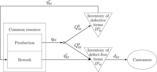
We consider an imperfect production process with a common resource for production and rework, i.e. according to Flapper et al. (2002), an in-line rework setting is assumed. The production system produces K products $(k=1,\dots ,K)$ over a finite planning horizon consisting of T discrete time periods $(t=1,\dots ,T)$. Figure 1 illustrates the underlying imperfect production process.

Figure 1. Integrated production and rework planning (cf. Inderfurth, Lindner, and Rachaniotis 2005 and Goerler and Voß 2016).

This figure visualizes the considered imperfect production process. The visualization includes a common resource for production and rework as well as separate inventories of defective and defect-free products.

The model assumptions for the stochastic capacitated lot sizing problem with rework of defective products (SCLSP-RW) are as follows:

• The imperfect production process is subject to a stochastic outcome of defective products. The random variable ${\mathrm{\Omega }}_{\mathrm{kt}}$ describes the proportion of defective items of product k in period t. The production quantity $q_{\mathrm{kt}}$ must be divided into defect-free $Q_{\mathrm{kt}}^g$ and defective products $Q_{\mathrm{kt}}^b$.

• The rework process is perfect, i.e, all defective products can be transformed into defect-free products.

• The product- and period-specific demand $d_{\mathrm{kt}}$ must be met according to a δ-service level.

• The period-specific capacity $c_t$ of the common resource is limited and can be extended by using overtime $o_t$ at overtime costs oc. The maximum amount of overtime is limited to a fraction α of the period-specific capacity $c_t$.

• The production of one unit of product k entails variable production costs $p{c}_k$ and requires production time $p{t}_k$. Similarly, reworking one unit of defective product k induces variable rework costs $p{c}_k^r$ and requires rework time $p{t}_k^r$.

• Both, the production and rework of product k require separate setup operations that induce different setup costs $s{c}_k$ and $s{c}_k^r$ as well as setup times $s{t}_k$ and $s{t}_k^r$. The setup operations are modelled by binary variables ${\gamma }_{\mathrm{kt}}$ and ${\gamma }_{\mathrm{kt}}^r$.

• Defect-free and defective products can be held in stock at inventory holding costs $h{c}_k$ and $h{c}_k^r$.

The planning situation is characterised by uncertainty related to the proportion of defective products. This uncertainty may lead to backlogs of defect-free products if the cumulated demand exceeds the cumulated quantity of defect-free products. To limit these expected backlogs $\text{E}\left[B{L}_{\mathrm{kt}}\right]$, we use the δ-service level proposed by Helber, Sahling, and Schimmelpfeng (2013). The δ-service level can be formally stated as follows: ${\delta }_k=1-\frac{\sum _{t\in \mathcal{T}}\text{E}\left[B{L}_{\mathrm{kt}}\right]}{\sum _{t\in \mathcal{T}}(T-t+1)\cdot d_{\mathrm{kt}}}\mathrm{\forall }k\in \mathcal{K}$In addition to backlogs of defect-free products, shortages of defective products may occur. In period t, the physical inventory of defective product k is increased by production $Q_{\mathrm{kt}}^b$ and decreased by planned rework quantities $q_{\mathrm{kt}}^r$. However, random quantities of defective products $Q_{\mathrm{kt}}^b$ manufactured in period t correspond to the random proportion of defective products ${\mathrm{\Omega }}_{\mathrm{kt}}$. Thus, it may occur that in some periods there are not enough defective products in stock to realise the planned rework quantity $q_{\mathrm{kt}}^r$. In this case, as shown in Figure 2, a shortfall of defective products may occur.

Figure 2. Development of the physical inventory of defective products (cf. Hilger, Sahling, and Tempelmeier 2016).

This graph shows an exemplary course of the physical inventory of defective products to illustrate the occurrence of shortfalls.

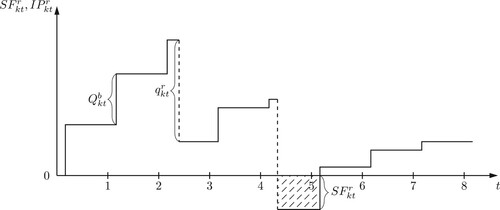
This random shortfall can be stated formally as follows: $S{F}_{\mathrm{kt}}^r=max\{0,q_{\mathrm{kt}}^r-(I{P}_{k,t-1}^r+Q_{\mathrm{kt}}^b\left)\right\}\mathrm{\forall }k\in \mathcal{K},t\in \mathcal{T}$Notably, such a shortfall results in an infeasible production and rework plan. Hilger, Sahling, and Tempelmeier (2016) address a similar situation in the area of stochastic integrated production and remanufacturing planning. Analogously, we use a constraint that limits the expected shortfall to a given small amount ϵ.

The objective of the SCLSP-RW is to find an integrated production and rework plan that takes into account the randomness of the proportion of defective products and minimises the expected total cost.

3.2. Model formulation

The generic SCLSP-RW can be formulated using the notation in Table 3:

Table 3. Notation for the SCLSP-RW.

Indices and index sets:
$k\in \mathcal{K}$	Set of products, $\mathcal{K}=\{1,\dots ,K\}$
$t\in \mathcal{T}$	Set of periods, $\mathcal{T}=\{1,\dots ,T\}$
Parameters:
α	Fraction of allowed overtime
${\delta }_k$	Target δ-service level for product k
ϵ	Small number
$c_t$	Capacity for production and rework in period t
$d_{\mathrm{kt}}$	Demand for product k in period t
$h{c}_k$	Cost for holding one defect-free unit of product k per period
$h{c}_k^r$	Cost for holding one defective unit of product k per period
$M_{\mathrm{kt}}$	Large number for product k in period t
oc	Overtime cost
$p{c}_k$	Production cost of product k
$p{c}_k^r$	Rework cost of product k
$p{t}_k$	Production time of product k
$p{t}_k^r$	Rework time of product k
$s{c}_k$	Setup cost for production of product k
$s{c}_k^r$	Setup cost for rework of product k
$s{t}_k$	Setup time for production of product k
$s{t}_k^r$	Setup time for rework of product k
Random variables:
${\mathrm{\Omega }}_{\mathrm{kt}}$	Proportion of defective items of product k in period t
$B{L}_{\mathrm{kt}}$	Backlog of defect-free items of product k at the end of period t
$I_{\mathrm{kt}}$	Net inventory of defect-free items of product k at the end of period t
$I_{\mathrm{kt}}^r$	Net inventory of defective items of product k at the end of period t
$I{P}_{\mathrm{kt}}$	Physical inventory of defect-free items of product k at the end of period t
$I{P}_{\mathrm{kt}}^r$	Physical inventory of defective items of product k at the end of period t
$Q_{\mathrm{kt}}^b$	Defective items of product k in period t
$Q_{\mathrm{kt}}^g$	Defect-free items of product k in period t
$S{F}_{\mathrm{kt}}^r$	Shortfall of defective items of product k in period t
Decision variables:
${\gamma }_{\mathrm{kt}}$	Binary setup variable for production of product k in period t
${\gamma }_{\mathrm{kt}}^r$	Binary setup variable for rework of product k in period t
$o_t$	Amount of overtime in period t
$q_{\mathrm{kt}}$	Production quantity of product k in period t
$q_{\mathrm{kt}}^r$	Rework quantity of product k in period t

Model SCLSP-RW: (1) $\begin{array}{rl}\text{min,}\text{E}\left[C\right]& =\sum _{k\in \mathcal{K}}\sum _{t\in \mathcal{T}}(s{c}_k\cdot {\gamma }_{\mathrm{kt}}+h{c}_k\cdot \text{E}[I{P}_{\mathrm{kt}}]+p{c}_k\cdot q_{\mathrm{kt}})\end{array}$(1) (2) $\begin{array}{rl}& +\sum _{k\in \mathcal{K}}\sum _{t\in \mathcal{T}}(s{c}_k^r\cdot {\gamma }_{\mathrm{kt}}^r+h{c}_k^r\cdot \text{E}[I{P}_{\mathrm{kt}}^r]+p{c}_k^r\cdot q_{\mathrm{kt}}^r)\end{array}$(2) (3) $\begin{array}{rl}& +\sum _{t\in \mathcal{T}}\mathrm{oc}\cdot o_t\end{array}$(3) subject to (4) $\begin{array}{rl}& I_{k,t-1}+Q_{\mathrm{kt}}^g+q_{\mathrm{kt}}^r-d_{\mathrm{kt}}=I_{\mathrm{kt}}\mathrm{\forall }k\in \mathcal{K},t\in \mathcal{T}\end{array}$(4) (5) $\begin{array}{rl}& I_{k,t-1}^r+Q_{\mathrm{kt}}^b-q_{\mathrm{kt}}^r=I_{\mathrm{kt}}^r\mathrm{\forall }k\in \mathcal{K},t\in \mathcal{T}\end{array}$(5) (6) $\begin{array}{rl}& I{P}_{\mathrm{kt}}=max\{0,I_{\mathrm{kt}}\}\mathrm{\forall }k\in \mathcal{K},t\in \mathcal{T}\end{array}$(6) (7) $\begin{array}{rl}& B{L}_{\mathrm{kt}}=max\{0,-I_{\mathrm{kt}}\}\mathrm{\forall }k\in \mathcal{K},t\in \mathcal{T}\end{array}$(7) (8) $\begin{array}{rl}& I{P}_{\mathrm{kt}}^r=max\{0,I_{\mathrm{kt}}^r\}\mathrm{\forall }k\in \mathcal{K},t\in \mathcal{T}\end{array}$(8) (9) $\begin{array}{rl}& S{F}_{\mathrm{kt}}^r=max\{0,-I_{\mathrm{kt}}^r\}\mathrm{\forall }k\in \mathcal{K},t\in \{t\mid {\gamma }_{\mathrm{kt}}^r=1;\\ & t=1,2,\dots ,T\}\end{array}$(9) (10) $\begin{array}{rl}& \sum _{t\in \mathcal{T}}\left(\text{E}\right[Q_{\mathrm{kt}}^g]+q_{\mathrm{kt}}^r)\ge \sum _{t\in \mathcal{T}}{d}_{\mathrm{kt}}\mathrm{\forall }k\in \mathcal{K}\end{array}$(10) (11) $\begin{array}{rl}& \sum _{t\in \mathcal{T}}\text{E}\left[B{L}_{\mathrm{kt}}\right]\le (1-{\delta }_k)\sum _{t\in \mathcal{T}}(T-t+1)\cdot d_{\mathrm{kt}}\mathrm{\forall }k\in \mathcal{K}\end{array}$(11) (12) $\begin{array}{rl}& \text{E}\left[S{F}_{\mathrm{kt}}^r\right]\le ϵ\mathrm{\forall }k\in \mathcal{K},t\in \mathcal{T}\end{array}$(12) (13) $\begin{array}{rl}& \sum _{k\in \mathcal{K}}(p{t}_k\cdot q_{\mathrm{kt}}+s{t}_k\cdot {\gamma }_{\mathrm{kt}}+p{t}_k^r\cdot q_{\mathrm{kt}}^r+s{t}_k^r\cdot {\gamma }_{\mathrm{kt}}^r)\le c_t+o_t\\ & \mathrm{\forall }t\in \mathcal{T}\end{array}$(13) (14) $\begin{array}{rl}& o_t\le \alpha \cdot c_t\mathrm{\forall }t\in \mathcal{T}\end{array}$(14) (15) $\begin{array}{rl}& q_{\mathrm{kt}}\le M_{\mathrm{kt}}\cdot {\gamma }_{\mathrm{kt}}\mathrm{\forall }k\in \mathcal{K},t\in \mathcal{T}\end{array}$(15) (16) $\begin{array}{rl}& q_{\mathrm{kt}}^r\le M_{\mathrm{kt}}\cdot {\gamma }_{\mathrm{kt}}^r\mathrm{\forall }k\in \mathcal{K},t\in \mathcal{T}\end{array}$(16) (17) $\begin{array}{rl}& Q_{\mathrm{kt}}^b={\mathrm{\Omega }}_{\mathrm{kt}}\cdot q_{\mathrm{kt}}\mathrm{\forall }k\in \mathcal{K},t\in \mathcal{T}\end{array}$(17) (18) $\begin{array}{rl}& Q_{\mathrm{kt}}^g=(1-{\mathrm{\Omega }}_{\mathrm{kt}})\cdot q_{\mathrm{kt}}\mathrm{\forall }k\in \mathcal{K},t\in \mathcal{T}\end{array}$(18) (19) $\begin{array}{rl}& q_{\mathrm{kt}},q_{\mathrm{kt}}^r\ge 0\mathrm{\forall }k\in \mathcal{K},t\in \mathcal{T}\end{array}$(19) (20) $\begin{array}{rl}& o_t\ge 0\mathrm{\forall }t\in \mathcal{T}\end{array}$(20) (21) $\begin{array}{rl}& {\gamma }_{\mathrm{kt}},{\gamma }_{\mathrm{kt}}^r\in \{0,1\}\mathrm{\forall }k\in \mathcal{K},t\in \mathcal{T}\end{array}$(21) The objective function (1(1) $\begin{array}{rl}\text{min,}\text{E}\left[C\right]& =\sum _{k\in \mathcal{K}}\sum _{t\in \mathcal{T}}(s{c}_k\cdot {\gamma }_{\mathrm{kt}}+h{c}_k\cdot \text{E}[I{P}_{\mathrm{kt}}]+p{c}_k\cdot q_{\mathrm{kt}})\end{array}$(1) )–(3(3) $\begin{array}{rl}& +\sum _{t\in \mathcal{T}}\mathrm{oc}\cdot o_t\end{array}$(3) ) aims to minimise the expected total sum of costs. The term (1(1) $\begin{array}{rl}\text{min,}\text{E}\left[C\right]& =\sum _{k\in \mathcal{K}}\sum _{t\in \mathcal{T}}(s{c}_k\cdot {\gamma }_{\mathrm{kt}}+h{c}_k\cdot \text{E}[I{P}_{\mathrm{kt}}]+p{c}_k\cdot q_{\mathrm{kt}})\end{array}$(1) ) contains the setup, expected inventory holding, and production costs related to the production process, whereas term (2(2) $\begin{array}{rl}& +\sum _{k\in \mathcal{K}}\sum _{t\in \mathcal{T}}(s{c}_k^r\cdot {\gamma }_{\mathrm{kt}}^r+h{c}_k^r\cdot \text{E}[I{P}_{\mathrm{kt}}^r]+p{c}_k^r\cdot q_{\mathrm{kt}}^r)\end{array}$(2) ) includes the costs regarding the rework process. The term (3(3) $\begin{array}{rl}& +\sum _{t\in \mathcal{T}}\mathrm{oc}\cdot o_t\end{array}$(3) ) contains overtime costs.

The inventory balance constraints for defect-free products are given by constraints (4(4) $\begin{array}{rl}& I_{k,t-1}+Q_{\mathrm{kt}}^g+q_{\mathrm{kt}}^r-d_{\mathrm{kt}}=I_{\mathrm{kt}}\mathrm{\forall }k\in \mathcal{K},t\in \mathcal{T}\end{array}$(4) ). Constraints (5(5) $\begin{array}{rl}& I_{k,t-1}^r+Q_{\mathrm{kt}}^b-q_{\mathrm{kt}}^r=I_{\mathrm{kt}}^r\mathrm{\forall }k\in \mathcal{K},t\in \mathcal{T}\end{array}$(5) ) represent the inventory balance constraints for defective products. Equations (6(6) $\begin{array}{rl}& I{P}_{\mathrm{kt}}=max\{0,I_{\mathrm{kt}}\}\mathrm{\forall }k\in \mathcal{K},t\in \mathcal{T}\end{array}$(6) ) and (7(7) $\begin{array}{rl}& B{L}_{\mathrm{kt}}=max\{0,-I_{\mathrm{kt}}\}\mathrm{\forall }k\in \mathcal{K},t\in \mathcal{T}\end{array}$(7) ) define the physical inventory and backlogs of defect-free products. Equations (8(8) $\begin{array}{rl}& I{P}_{\mathrm{kt}}^r=max\{0,I_{\mathrm{kt}}^r\}\mathrm{\forall }k\in \mathcal{K},t\in \mathcal{T}\end{array}$(8) ) and (9(9) $\begin{array}{rl}& S{F}_{\mathrm{kt}}^r=max\{0,-I_{\mathrm{kt}}^r\}\mathrm{\forall }k\in \mathcal{K},t\in \{t\mid {\gamma }_{\mathrm{kt}}^r=1;\\ & t=1,2,\dots ,T\}\end{array}$(9) ) define the physical inventory and shortfalls of defective products, respectively.

Constraints (10(10) $\begin{array}{rl}& \sum _{t\in \mathcal{T}}\left(\text{E}\right[Q_{\mathrm{kt}}^g]+q_{\mathrm{kt}}^r)\ge \sum _{t\in \mathcal{T}}{d}_{\mathrm{kt}}\mathrm{\forall }k\in \mathcal{K}\end{array}$(10) ) enforce that at least the cumulated demand of defect-free products is met by the cumulated expected quantity of defect-free products and reworked quantities. Constraints (11(11) $\begin{array}{rl}& \sum _{t\in \mathcal{T}}\text{E}\left[B{L}_{\mathrm{kt}}\right]\le (1-{\delta }_k)\sum _{t\in \mathcal{T}}(T-t+1)\cdot d_{\mathrm{kt}}\mathrm{\forall }k\in \mathcal{K}\end{array}$(11) ) limit the expected backlogs according to the target δ-service level. Furthermore, constraints (12(12) $\begin{array}{rl}& \text{E}\left[S{F}_{\mathrm{kt}}^r\right]\le ϵ\mathrm{\forall }k\in \mathcal{K},t\in \mathcal{T}\end{array}$(12) ) ensure that rework of defective quantities is planned only if the expected physical inventory is sufficient. The capacity for the common production and rework resource is limited by constraints (13(13) $\begin{array}{rl}& \sum _{k\in \mathcal{K}}(p{t}_k\cdot q_{\mathrm{kt}}+s{t}_k\cdot {\gamma }_{\mathrm{kt}}+p{t}_k^r\cdot q_{\mathrm{kt}}^r+s{t}_k^r\cdot {\gamma }_{\mathrm{kt}}^r)\le c_t+o_t\\ & \mathrm{\forall }t\in \mathcal{T}\end{array}$(13) ). Constraints (14(14) $\begin{array}{rl}& o_t\le \alpha \cdot c_t\mathrm{\forall }t\in \mathcal{T}\end{array}$(14) ) ensure that the planned amount of overtime does not exceed the allowed maximum. The production and rework quantities $q_{\mathrm{kt}}$ and $q_{\mathrm{kt}}^r$ are linked to the binary setup variables ${\gamma }_{\mathrm{kt}}$ and ${\gamma }_{\mathrm{kt}}^r$ according to constraints (15(15) $\begin{array}{rl}& q_{\mathrm{kt}}\le M_{\mathrm{kt}}\cdot {\gamma }_{\mathrm{kt}}\mathrm{\forall }k\in \mathcal{K},t\in \mathcal{T}\end{array}$(15) ) and (16(16) $\begin{array}{rl}& q_{\mathrm{kt}}^r\le M_{\mathrm{kt}}\cdot {\gamma }_{\mathrm{kt}}^r\mathrm{\forall }k\in \mathcal{K},t\in \mathcal{T}\end{array}$(16) ).

Notably, in the literature, there exist various reformulations to replace the parameter $M_{\mathrm{kt}}$ in constraints (15(15) $\begin{array}{rl}& q_{\mathrm{kt}}\le M_{\mathrm{kt}}\cdot {\gamma }_{\mathrm{kt}}\mathrm{\forall }k\in \mathcal{K},t\in \mathcal{T}\end{array}$(15) ) and (16(16) $\begin{array}{rl}& q_{\mathrm{kt}}^r\le M_{\mathrm{kt}}\cdot {\gamma }_{\mathrm{kt}}^r\mathrm{\forall }k\in \mathcal{K},t\in \mathcal{T}\end{array}$(16) ) to strengthen the LP relaxation, see e.g. Retel Helmrich et al. (2014), Cunha and Melo (2016), and Syed Ali et al. (2018). However, Helber and Sahling (2010) pointed out that these reformulations result in an increased number of additional variables, so that the computational time of the heuristic proposed in Section 4.2 also increases substantially. Thus, the standard formulation is still used in the following.

The amounts of defect-free and defective products of a lot are defined by the random proportion of defective products ${\mathrm{\Omega }}_{\mathrm{kt}}$. In period t, the random quantity of defective items $Q_{\mathrm{kt}}^b$ related to production quantity $q_{\mathrm{kt}}$ is derived by restrictions (17(17) $\begin{array}{rl}& Q_{\mathrm{kt}}^b={\mathrm{\Omega }}_{\mathrm{kt}}\cdot q_{\mathrm{kt}}\mathrm{\forall }k\in \mathcal{K},t\in \mathcal{T}\end{array}$(17) ) for product k. The random quantity of defect-free items $Q_{\mathrm{kt}}^g$ is defined by constraints (18(18) $\begin{array}{rl}& Q_{\mathrm{kt}}^g=(1-{\mathrm{\Omega }}_{\mathrm{kt}})\cdot q_{\mathrm{kt}}\mathrm{\forall }k\in \mathcal{K},t\in \mathcal{T}\end{array}$(18) ). These items can be used to satisfy demand directly. Finally, constraints (19(19) $\begin{array}{rl}& q_{\mathrm{kt}},q_{\mathrm{kt}}^r\ge 0\mathrm{\forall }k\in \mathcal{K},t\in \mathcal{T}\end{array}$(19) ) and (20(20) $\begin{array}{rl}& o_t\ge 0\mathrm{\forall }t\in \mathcal{T}\end{array}$(20) ) define production and rework quantities and overtime variables as nonnegative. Constraints (21(21) $\begin{array}{rl}& {\gamma }_{\mathrm{kt}},{\gamma }_{\mathrm{kt}}^r\in \{0,1\}\mathrm{\forall }k\in \mathcal{K},t\in \mathcal{T}\end{array}$(21) ) define the setup variables as binary.

Currently, no solution approach exist to directly solve the generic nonlinear SCLSP-RW. Thus, a sample average approach is applied to approximate the SCLSP-RW.

3.3. Approximation of SCLSP-RW via sample averages

In the sample average approach, cf. Kleywegt, Shapiro, and Homem-de-Melo (2002) and Helber, Sahling, and Schimmelpfeng (2013), random variables are represented by samples of randomly generated scenarios $(s=1,2,\dots ,S)$. In our case, each scenario corresponds to a possible realisation of the random proportion of defective products. In advance, the scenario-specific proportion of defective products ${\omega }_{\mathrm{kts}}$ is determined following the distribution information of the random variable ${\mathrm{\Omega }}_{\mathrm{kt}}$.

Since the scenario-specific proportion of defective products ${\omega }_{\mathrm{kts}}$ is generated based on the underlying probability distribution of ${\mathrm{\Omega }}_{\mathrm{kt}}$, the sample average over all scenarios approximately matches the expected proportion of defective products $\text{E}\left[{\mathrm{\Omega }}_{\mathrm{kt}}\right]\approx \sum _{s\in \mathcal{S}}\frac{{\omega }_{\mathrm{kts}}}{|\mathcal{S}|}\mathrm{\forall }k\in \mathcal{K},t\in \mathcal{T}$Starting from a given proportion of defectives ${\omega }_{\mathrm{kts}}$, the scenario-specific quantities of defective $q_{\mathrm{kts}}^b$ and defect-free products $q_{\mathrm{kts}}^g$ can be determined for production quantity $q_{\mathrm{kt}}$: (17′) $\begin{array}{rl}& q_{\mathrm{kts}}^b={\omega }_{\mathrm{kts}}\cdot q_{\mathrm{kt}}\mathrm{\forall }k\in \mathcal{K},t\in \mathcal{T},s\in \mathcal{S}\\ & q_{\mathrm{kts}}^g=(1-{\omega }_{\mathrm{kts}})\cdot q_{\mathrm{kt}}\mathrm{\forall }k\in \mathcal{K},t\in \mathcal{T},s\in \mathcal{S}18{\$}^{\mathrm{\prime }}\$\end{array}$(17′) Using these scenario-specific quantities of defect-free products $q_{\mathrm{kts}}^g$, scenario-specific net inventories $i_{\mathrm{kts}}$, physical inventories $i{p}_{\mathrm{kts}}$ and backlogs $b{l}_{\mathrm{kts}}$ can be determined for rework quantity $q_{\mathrm{kt}}^r$ as follows: $\begin{array}{rl}& i_{k,t-1,s}+q_{\mathrm{kts}}^g+q_{\mathrm{kt}}^r-d_{\mathrm{kt}}=i_{\mathrm{kts}}\mathrm{\forall }k\in \mathcal{K},t\in \mathcal{T},s\in \mathcal{S}4{\$}^{\mathrm{\prime }}\$\\ & i{p}_{\mathrm{kts}}\ge i_{\mathrm{kts}}\mathrm{\forall }k\in \mathcal{K},t\in \mathcal{T},s\in \mathcal{S}6{\$}^{\mathrm{\prime }}\$\\ & b{l}_{\mathrm{kts}}\ge -i_{\mathrm{kts}}\mathrm{\forall }k\in \mathcal{K},t\in \mathcal{T},s\in \mathcal{S}7{\$}^{\mathrm{\prime }}\$\end{array}$Since the sample average over all scenarios approximates the expected proportion of defective products $\text{E}\left[{\mathrm{\Omega }}_{\mathrm{kt}}\right]$, the expected physical inventory $\text{E}\left[I{P}_{\mathrm{kt}}\right]$ can also be approximated by sample averages: $\begin{array}{r}\text{E}\left[I{P}_{\mathrm{kt}}\right]\approx \sum _{s\in \mathcal{S}}\frac{i{p}_{\mathrm{kts}}}{|\mathcal{S}|}\mathrm{\forall }k\in \mathcal{K},t\in \mathcal{T}\end{array}$Similarly, the expected backlog $\text{E}\left[B{L}_{\mathrm{kt}}\right]$, the expected quantity of defect-free products $\text{E}\left[Q_{\mathrm{kt}}^g\right]$, the expected physical inventory $\text{E}\left[I{P}_{\mathrm{kt}}^r\right]$ and the expected shortfall $\text{E}\left[S{F}_{\mathrm{kt}}^r\right]$ of defective products are approximated by sample averages.

On the basis of these scenario-based modifications and the additional notation in Table 4, the generic nonlinear SCLSP-RW can be approximated as follows.

Table 4. Additional notation for SCLSP-RW${}^{\mathrm{SAA}}$.

Indices and index sets:
$s\in \mathcal{S}$	Set of scenarios, $\mathcal{S}=\{1,\dots ,S\}$
Scenario-specific parameters:
${\omega }_{\mathrm{kts}}$	Proportion of defective items of product k in period t and scenario s
Scenario-specific decision variables:
$b{l}_{\mathrm{kts}}$	Backlog of defect-free items of product k in period t and scenario s
$i_{\mathrm{kts}}$	Net inventory of defect-free items of product k at the end of period t in scenario s
$i_{\mathrm{kts}}^r$	Net inventory of defective items of product k at the end of period t in scenario s
$i{p}_{\mathrm{kts}}$	Physical inventory of defect-free items of product k at the end of period t in scenario s
$i{p}_{\mathrm{kts}}^r$	Physical inventory of defective items of product k at the end of period t in scenario s
$q_{\mathrm{kts}}^b$	Defective items of product k in period t and scenario s
$q_{\mathrm{kts}}^g$	Defect-free items of product k in period t and scenario s
$s{f}_{\mathrm{kts}}^r$	Shortfall of defective items of product k in period t and scenario s

Model SCLSP-RW${}^{\mathrm{SAA}}$: $\begin{array}{rl}\text{min,}\text{E}\left[C\right]& =\sum _{k\in \mathcal{K}}\sum _{t\in \mathcal{T}}(\phantom{\sum _{s\in \mathcal{S}}}s{c}_k\cdot {\gamma }_{\mathrm{kt}}+h{c}_k\\ & \cdot \sum _{s\in \mathcal{S}}\frac{i{p}_{\mathrm{kts}}}{|\mathcal{S}|}+p{c}_k\cdot q_{\mathrm{kt}})1{\$}^{\mathrm{\prime }}\$\\ & +\sum _{k\in \mathcal{K}}\sum _{t\in \mathcal{T}}(\phantom{\sum _{s\in \mathcal{S}}}s{c}_k^r\cdot {\gamma }_{\mathrm{kt}}^r+h{c}_k^r\\ & \cdot \sum _{s\in \mathcal{S}}\frac{i{p}_{\mathrm{kts}}^r}{|\mathcal{S}|}+p{c}_k^r\cdot q_{\mathrm{kt}}^r)2{\$}^{\mathrm{\prime }}\$\\ & +\sum _{t\in \mathcal{T}}\mathrm{oc}\cdot o_{t}3{\$}^{\mathrm{\prime }}\$\end{array}$subject to (4(4) $\begin{array}{rl}& I_{k,t-1}+Q_{\mathrm{kt}}^g+q_{\mathrm{kt}}^r-d_{\mathrm{kt}}=I_{\mathrm{kt}}\mathrm{\forall }k\in \mathcal{K},t\in \mathcal{T}\end{array}$(4) '), (6(6) $\begin{array}{rl}& I{P}_{\mathrm{kt}}=max\{0,I_{\mathrm{kt}}\}\mathrm{\forall }k\in \mathcal{K},t\in \mathcal{T}\end{array}$(6) '), (7(7) $\begin{array}{rl}& B{L}_{\mathrm{kt}}=max\{0,-I_{\mathrm{kt}}\}\mathrm{\forall }k\in \mathcal{K},t\in \mathcal{T}\end{array}$(7) '), (13(13) $\begin{array}{rl}& \sum _{k\in \mathcal{K}}(p{t}_k\cdot q_{\mathrm{kt}}+s{t}_k\cdot {\gamma }_{\mathrm{kt}}+p{t}_k^r\cdot q_{\mathrm{kt}}^r+s{t}_k^r\cdot {\gamma }_{\mathrm{kt}}^r)\le c_t+o_t\\ & \mathrm{\forall }t\in \mathcal{T}\end{array}$(13) )–(16(16) $\begin{array}{rl}& q_{\mathrm{kt}}^r\le M_{\mathrm{kt}}\cdot {\gamma }_{\mathrm{kt}}^r\mathrm{\forall }k\in \mathcal{K},t\in \mathcal{T}\end{array}$(16) ), (17(17) $\begin{array}{rl}& Q_{\mathrm{kt}}^b={\mathrm{\Omega }}_{\mathrm{kt}}\cdot q_{\mathrm{kt}}\mathrm{\forall }k\in \mathcal{K},t\in \mathcal{T}\end{array}$(17) '), (18(18) $\begin{array}{rl}& Q_{\mathrm{kt}}^g=(1-{\mathrm{\Omega }}_{\mathrm{kt}})\cdot q_{\mathrm{kt}}\mathrm{\forall }k\in \mathcal{K},t\in \mathcal{T}\end{array}$(18) '), (19(19) $\begin{array}{rl}& q_{\mathrm{kt}},q_{\mathrm{kt}}^r\ge 0\mathrm{\forall }k\in \mathcal{K},t\in \mathcal{T}\end{array}$(19) )–(21(21) $\begin{array}{rl}& {\gamma }_{\mathrm{kt}},{\gamma }_{\mathrm{kt}}^r\in \{0,1\}\mathrm{\forall }k\in \mathcal{K},t\in \mathcal{T}\end{array}$(21) ) and $\begin{array}{rl}& i_{k,t-1,s}^r+q_{\mathrm{kts}}^b-q_{\mathrm{kt}}^r=i_{\mathrm{kts}}^r\mathrm{\forall }k\in \mathcal{K},t\in \mathcal{T},s\in \mathcal{S}5{\$}^{\mathrm{\prime }}\$\\ & i{p}_{\mathrm{kts}}^r\ge i_{\mathrm{kts}}^r\mathrm{\forall }k\in \mathcal{K},t\in \mathcal{T},s\in \mathcal{S}8{\$}^{\mathrm{\prime }}\$\\ & s{f}_{\mathrm{kts}}^r\ge -i_{\mathrm{kts}}^r\mathrm{\forall }k\in \mathcal{K},t\in \{t\mid {\gamma }_{\mathrm{kt}}^r=1;\\ & t=1,2,\dots ,T\},s\in \mathcal{S}9{\$}^{\mathrm{\prime }}\$\\ & \sum _{t\in \mathcal{T}}(\sum _{s\in \mathcal{S}}\frac{q_{\mathrm{kts}}^g}{|\mathcal{S}|}+q_{\mathrm{kt}}^r)\ge \sum _{t\in \mathcal{T}}{d}_{\mathrm{kt}}\mathrm{\forall }k\in \mathcal{K}10{\$}^{\mathrm{\prime }}\$\\ & \sum _{t\in \mathcal{T}}\sum _{s\in \mathcal{S}}\frac{b{l}_{\mathrm{kts}}}{|\mathcal{S}|}\le (1-{\delta }_k)\sum _{t\in \mathcal{T}}(T-t+1)\cdot d_{\mathrm{kt}}\\ & \mathrm{\forall }k\in \mathcal{K}11{\$}^{\mathrm{\prime }}\$\\ & \sum _{s\in \mathcal{S}}\frac{s{f}_{\mathrm{kts}}^r}{|\mathcal{S}|}\le ϵ\mathrm{\forall }k\in \mathcal{K},t\in \mathcal{T}12{\$}^{\mathrm{\prime }}\$\\ & b{l}_{\mathrm{kts}},i{p}_{\mathrm{kts}},i{p}_{\mathrm{kts}}^r,q_{\mathrm{kts}}^b,q_{\mathrm{kts}}^g,s{f}_{\mathrm{kts}}^r\ge 0\\ & \mathrm{\forall }k\in \mathcal{K},t\in \mathcal{T},s\in \mathcal{S}22\end{array}$ The expected values of the physical inventory of defect-free $\text{E}\left[I{P}_{\mathrm{kt}}\right]$ and defective products $\text{E}\left[I{P}_{\mathrm{kt}}^r\right]$ are substituted by the corresponding sample averages in the objective function (1(1) $\begin{array}{rl}\text{min,}\text{E}\left[C\right]& =\sum _{k\in \mathcal{K}}\sum _{t\in \mathcal{T}}(s{c}_k\cdot {\gamma }_{\mathrm{kt}}+h{c}_k\cdot \text{E}[I{P}_{\mathrm{kt}}]+p{c}_k\cdot q_{\mathrm{kt}})\end{array}$(1) ') and (2(2) $\begin{array}{rl}& +\sum _{k\in \mathcal{K}}\sum _{t\in \mathcal{T}}(s{c}_k^r\cdot {\gamma }_{\mathrm{kt}}^r+h{c}_k^r\cdot \text{E}[I{P}_{\mathrm{kt}}^r]+p{c}_k^r\cdot q_{\mathrm{kt}}^r)\end{array}$(2) '). Scenario-specific inventory balance constraints are defined by (4(4) $\begin{array}{rl}& I_{k,t-1}+Q_{\mathrm{kt}}^g+q_{\mathrm{kt}}^r-d_{\mathrm{kt}}=I_{\mathrm{kt}}\mathrm{\forall }k\in \mathcal{K},t\in \mathcal{T}\end{array}$(4) ') and (5(5) $\begin{array}{rl}& I_{k,t-1}^r+Q_{\mathrm{kt}}^b-q_{\mathrm{kt}}^r=I_{\mathrm{kt}}^r\mathrm{\forall }k\in \mathcal{K},t\in \mathcal{T}\end{array}$(5) '). Constraints (6(6) $\begin{array}{rl}& I{P}_{\mathrm{kt}}=max\{0,I_{\mathrm{kt}}\}\mathrm{\forall }k\in \mathcal{K},t\in \mathcal{T}\end{array}$(6) ') to (9(9) $\begin{array}{rl}& S{F}_{\mathrm{kt}}^r=max\{0,-I_{\mathrm{kt}}^r\}\mathrm{\forall }k\in \mathcal{K},t\in \{t\mid {\gamma }_{\mathrm{kt}}^r=1;\\ & t=1,2,\dots ,T\}\end{array}$(9) ') define the scenario-specific physical inventory and backlog of defect-free products and the scenario-specific physical inventory and shortfall of defective products. The expected value of defect-free products $\text{E}\left[Q_{\mathrm{kt}}^g\right]$, expected backlog $\text{E}\left[B{L}_{\mathrm{kt}}\right]$, and expected shortfall $\text{E}\left[S{F}_{\mathrm{kt}}^r\right]$ are replaced by sample averages in (10(10) $\begin{array}{rl}& \sum _{t\in \mathcal{T}}\left(\text{E}\right[Q_{\mathrm{kt}}^g]+q_{\mathrm{kt}}^r)\ge \sum _{t\in \mathcal{T}}{d}_{\mathrm{kt}}\mathrm{\forall }k\in \mathcal{K}\end{array}$(10) ') to (12(12) $\begin{array}{rl}& \text{E}\left[S{F}_{\mathrm{kt}}^r\right]\le ϵ\mathrm{\forall }k\in \mathcal{K},t\in \mathcal{T}\end{array}$(12) '). Constraints (22) are the nonnegativity constraints for the scenario-specific variables.

Since the setup pattern and production and rework quantities are not determined for a specific scenario, the solution of the SCLSP-RW${}^{\mathrm{SAA}}$ yields a robust production and rework plan at minimal total expected costs. This robust plan meets the capacity restrictions and the target δ-service level on average.

4. A flexible planning approach based on multistage stochastic programming

4.1. Idea

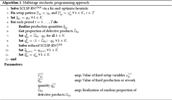
Following the static-dynamic uncertainty strategy of Bookbinder and Tan (1988), we present a multistage stochastic programming approach to cope with the random proportion of defective products in integrated lot sizing and rework planning. This approach enables a recourse, i.e. decisions on period-specific production and rework quantities can be revisited in each period and adjusted if necessary. In the first stage, setup decisions are determined and then fixed for the entire planning horizon. In subsequent stages, based on the fixed setup pattern, adjustments of production and rework quantities are allowed according to the realised proportion of defective product units of a production lot in a rolling horizon fashion.

4.2. Determine a robust setup pattern via fix-and-optimize

Assuming a perfect production process, the proportion of defective products is 0% and is thus known with certainty. In this case, since there are only defect-free products, there is no need for a rework option. Furthermore, if the target service level requirement is 100%, the SCLSP-RW${}^{\mathrm{SAA}}$ can be reduced to the well-known capacitated lot sizing problem (CLSP), which is proven to be $\mathcal{NP}$-hard; see Florian, Lenstra, and Kan (1980). Thus, the SCLSP-RW${}^{\mathrm{SAA}}$ is also $\mathcal{NP}$-hard and a suitable heuristic solution approach is required.

Due to the flexibility of MP-based solution approaches, we apply a variant of the fix-and-optimize heuristic proposed by Helber and Sahling (2010) to determine a robust setup pattern in the first stage. The underlying idea of the heuristic is to iteratively solve a series of subproblems derived from the original SCLSP-RW${}^{\mathrm{SAA}}$ using a product-oriented decomposition strategy. Thus, in each subproblem, only the binary setup variables ${\gamma }_{\mathrm{kt}}$ and ${\gamma }_{\mathrm{kt}}^r$ are solved to (sub)optimality for exactly one product k over the complete planning horizon ($t=1,\dots ,T$), while the remaining binary variables are fixed at values determined in the solution of previously treated subproblems. In addition, the optimal values for all real-valued decision variables are determined in each subproblem. The resulting subproblems are solved by the standard MIP solver CPLEX. This approach substantially reduces the numerical effort required to solve each subproblem to (sub)optimality, since the number of simultaneously treated binary variables is significantly reduced. As suggested by Helber and Sahling (2010), we start with a lot-for-lot initial solution, i.e. all binary variables ${\gamma }_{\mathrm{kt}}$ and ${\gamma }_{\mathrm{kt}}^r$ are set to 1. Subsequently, the products are treated in ascending indexing order, starting with the first product. The solution process is terminated when all products have been treated once. The resulting setup pattern is then fixed and serves as the basis for the flexible planning approach that allows adjustments to production and rework quantities in subsequent stages.

4.3. Adaptation of production and rework quantities

Solving the SCLSP-RW${}^{\mathrm{SAA}}$ results in a robust and stable production and rework plan for the complete planning horizon. However, it may be useful to modify the production and rework plan once the proportion of defective products in a production lot is known. Therefore, a multistage stochastic programming approach is proposed to allow flexibility, i.e. period-specific adjustments of the production and rework quantities.

As explained previously, in the first stage, the SCLSP-RW${}^{\mathrm{SAA}}$ is solved to generate a setup pattern that minimises the total sum of expected costs according to (1(1) $\begin{array}{rl}\text{min,}\text{E}\left[C\right]& =\sum _{k\in \mathcal{K}}\sum _{t\in \mathcal{T}}(s{c}_k\cdot {\gamma }_{\mathrm{kt}}+h{c}_k\cdot \text{E}[I{P}_{\mathrm{kt}}]+p{c}_k\cdot q_{\mathrm{kt}})\end{array}$(1) '), (2(2) $\begin{array}{rl}& +\sum _{k\in \mathcal{K}}\sum _{t\in \mathcal{T}}(s{c}_k^r\cdot {\gamma }_{\mathrm{kt}}^r+h{c}_k^r\cdot \text{E}[I{P}_{\mathrm{kt}}^r]+p{c}_k^r\cdot q_{\mathrm{kt}}^r)\end{array}$(2) ') and (3(3) $\begin{array}{rl}& +\sum _{t\in \mathcal{T}}\mathrm{oc}\cdot o_t\end{array}$(3) ). This setup pattern is fixed, i.e. all binary setup variables ${\gamma }_{\mathrm{kt}}$ and ${\gamma }_{\mathrm{kt}}^r$ cannot be changed afterwards.

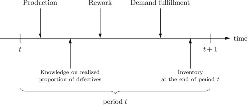
Each subsequent stage corresponds to a single period t. According to Figure 3, which describes the sequence of events in each period t, production quantities $q_{\mathrm{kt}}$ are first manufactured on the common resource. It is assumed that the realised proportion of defective products ${\tilde{\mathrm{\Omega }}}_{\mathrm{kt}}$ is known immediately after the production of a lot, i.e. the quantities of defect-free $q_{\mathrm{kt}}^g$ and defective items $q_{\mathrm{kt}}^b$ are available. Subsequently, a reduced SCLSP-RW${}_t^{\mathrm{SAA}}$ is solved considering only the current and subsequent periods ($\tau =t,\dots ,T$) by taking information regarding physical inventories, backlogs and shortfalls up to this period into account. In the reduced SCLSP-RW${}_t^{\mathrm{SAA}}$, a consideration of scenarios is necessary only for future periods ($\tau =t+1,\dots ,T$). In addition to the setup pattern, which remains fixed, the updated quantities of defective $q_{\mathrm{kt}}^b$ and defect-free products $q_{\mathrm{kt}}^g$ of the current period t are incorporated. This provides the flexibility to adjust rework quantities for the current and subsequent periods. The same applies to the production quantities of future periods ($\tau =t+1,\dots ,T$). The multistage stochastic programming approach is outlined in Algorithm 1.

Figure 3. Sequence of events in period t (cf. Kirste 2017).

This figure shows the timing of the production, the knowledge on the realized proportion of defectives, the rework, and the fulfilment of the demand in the period t.

5. Numerical analysis

5.1. Description of test design

For our numerical study, we defined two problem classes (PC) with different numbers of products and periods. In PC 1, K = 5 products and T = 10 periods were considered. PC 2 contained K = 20 products and T = 16 periods. There were 144 test instances in each PC.

The generation of test instances is described in detail below. By systematically varying various parameters, the test instances were defined. Table 5 provides an overview of these parameters.

Table 5. Varying parameters.

Number of products and periods	$\left(K/T\right)\in \left\{\right(5/10),(20/16\left)\right\}$
Mean proportion of defective products	${\overline{\mathrm{\Omega }}}_k\in \{0.02,0.04,0.06\}$
Range of the proportion of defective products	${\mathrm{Range}}_{\mathrm{\Omega }}\in \{\pm 0.1\cdot {\overline{\mathrm{\Omega }}}_k,\pm 0.3\cdot {\overline{\mathrm{\Omega }}}_k\}$
Variability of the demand	$V{C}_d\in \{0.2,0.3\}$
Capacity utilisation	$\mathrm{Util}\in \{0.6,0.9\}$
Time between orders	$\mathrm{TBO}\in \{1,2,4\}$
Target service level	$\delta \in \{0.9,0.95\}$

The demand data were created by randomly generating the average demand ${\overline{d}}_k$ following a uniform distribution within the interval [50,100]. The average demand ${\overline{d}}_k$ was then used to generate two dynamic demand series following a normal distribution. The two series differed in the variability of demand $V{C}_d$ (see Table 5). The proportion of defective products was also randomly generated following a uniform and a triangular distribution with a mean proportion of defective products ${\overline{\mathrm{\Omega }}}_k$ and a range ${\mathrm{Range}}_{\mathrm{\Omega }}$ (see Table 5).

For an overview of the constant parameter values, see Table 6.

Table 6. Constant parameter values.

Production cost of product k	$p{c}_k=4$
Rework cost of product k	$p{c}_k^r=1.5$
Production time of product k	$p{t}_k=0.08$
Rework time of product k	$p{t}_k^r=0.03$
Setup cost for production of product k	$s{c}_k=12.5$
Setup cost for rework of product k	$s{c}_k^r=3.125$
Setup time for production of product k	$s{t}_k=0.25$
Setup time for rework of product k	$s{t}_k^r=0.0625$
Fraction of allowed overtime	$\alpha =0.1$
Small number	$ϵ=0.01$
Overtime cost	oc = 75

We assume that the setup costs for the production process are higher than those for the rework process; see Widyana and Wee (2012). Furthermore, the setup cost is proportional to the setup time; see Jamal, Sarker, and Mondal (2004).

According to Tempelmeier (2011), the holding cost $h{c}_k$ is calculated by (23) $\begin{array}{r}h{c}_k=\frac{2\cdot s{c}_k}{{\overline{d}}_k\cdot \mathrm{TB}{O}^2}\mathrm{\forall }k\in \mathcal{K}\end{array}$(23) based on the setup cost $s{c}_k$, the average demand ${\overline{d}}_k$ and the time between orders TBO (see Table 5). Furthermore, it is assumed that the cost of holding defective and defect-free items is the same; see Goerler and Voß (2016).

The production cost $p{c}_k$ is proportional to the production time, see Sahling (2010). The same applies to rework cost and time. According to Goerler and Voß (2016), we assume that the production time is higher than the rework time.

The capacity for production and rework in period t is calculated according to Equations (24(24) $\begin{array}{rl}{c}_t& =\frac{1}{\mathrm{Util}}\cdot \sum _{k\in \mathcal{K}}(p{t}_k\cdot {\overline{d}}_k+s{t}_k+p{t}_k^r\cdot {\overline{d}}_k\cdot {\overline{\mathrm{\Omega }}}_k+s{t}_k^r)\\ & \mathrm{\forall }t\in \mathcal{T}\end{array}$(24) ). (24) $\begin{array}{rl}{c}_t& =\frac{1}{\mathrm{Util}}\cdot \sum _{k\in \mathcal{K}}(p{t}_k\cdot {\overline{d}}_k+s{t}_k+p{t}_k^r\cdot {\overline{d}}_k\cdot {\overline{\mathrm{\Omega }}}_k+s{t}_k^r)\\ & \mathrm{\forall }t\in \mathcal{T}\end{array}$(24) It is assumed that the capacity is sufficient to produce the average demand of each product k and to rework the mean defective products resulting from these production quantities in period t. In addition, a production and rework setup is assumed for each product k in period t. The capacity is extended by the utilisation Util to ensure a feasible solution. The parameter $M_{\mathrm{kt}}$ is calculated according to Equations (25): (25) $\begin{array}{r}{M}_{\mathrm{kt}}=\frac{2\cdot c_t}{min\{p{t}_k,p{t}_k^r\}}\mathrm{\forall }k\in \mathcal{K},t\in \mathcal{T}.\end{array}$(25) Following, e.g. Sarkar et al. (2014), Kang et al. (2017) and Asadkhani, Mokhtari, and Tahmasebpoor (2022), we assume that the random variable ${\mathrm{\Omega }}_{\mathrm{kt}}$ describing the proportion of defective products is uniformly distributed. Furthermore, we investigate the influence of a triangularly distributed random variable ${\mathrm{\Omega }}_{\mathrm{kt}}$, as assumed, e.g. in Sarkar et al. (2014) and Kang et al. (2017). For the values of the mean proportion of defective products, we follow a survey by Lay, Dreher, and Kinkel (1996), which found that the average proportion of defective products among 1,305 companies in the German capital goods industry was 4.9%. Comparable values can also be found in the literature; see e.g. Sarkar et al. (2014), Goerler and Voß (2016), Goerler, Lalla-Ruiz, and Voß (2020), and Asadkhani, Mokhtari, and Tahmasebpoor (2022). We analyse different ranges of the proportion of defective products. Ranges found in the literature are, e.g. $\pm 0.4\cdot {\overline{\mathrm{\Omega }}}_k$ (see Sarkar et al. 2014) or $\pm 0.5\cdot {\overline{\mathrm{\Omega }}}_k$ (see Asadkhani, Mokhtari, and Tahmasebpoor 2022). To cover different planning scenarios and the influence of different ranges, we used different values: a lower range $\pm 0.1\cdot {\overline{\mathrm{\Omega }}}_k$, a medium range $\pm 0.3\cdot {\overline{\mathrm{\Omega }}}_k$, and in Section 5.4 a higher range $\pm 0.5\cdot {\overline{\mathrm{\Omega }}}_k$. Additional analysed parameters are represented by the coefficient of variation of the demand $V{C}_d$, the capacity utilisation, the time between orders (TBO) used to determine holding costs, and the target service level δ.

Regarding the generation of scenarios, Helber, Sahling, and Schimmelpfeng (2013) state that the descriptive sampling proposed by Saliby (1990) is superior to a simple random sampling approach. Consequently, we use descriptive sampling to reduce the number of scenarios considered and thus the numerical effort required to solve the scenario-based approximation model. Preliminary numerical tests have shown that ten scenarios are sufficient.

Our numerical investigations were performed on an Intel Core CPU with six 2.90 GHz threads and 16 GB of RAM. We implemented the model formulation of the SCLSP-RW${}^{\mathrm{SAA}}$ and the multistage stochastic programming approach in GAMS 36.2.0. In the fix-and-optimize heuristic, each subproblem was solved up to an integrality gap of 0.1% using the standard MIP solver CPLEX (ver. 20.1.0.1). The remaining linear programs of the reduced SCLSP-RW${}^{\mathrm{SAA}}$ were also solved with CPLEX.

5.2. Simulation-based analysis

5.2.1. Uniformly distributed proportion of defective products

As described above, production and rework quantities can be adapted during the multistage stochastic programming approach. To analyse the advantage of flexible planning, a simulation study with 1,000 replications was conducted. For each replication, which consists of different realizations of the random proportion of defective products, the flexible approach is applied iteratively. Based on the fixed setup pattern, future production and rework quantities can be adjusted in each period after the proportion of defective items in a lot is known. We use slack variables in the demand constraints (10(10) $\begin{array}{rl}& \sum _{t\in \mathcal{T}}\left(\text{E}\right[Q_{\mathrm{kt}}^g]+q_{\mathrm{kt}}^r)\ge \sum _{t\in \mathcal{T}}{d}_{\mathrm{kt}}\mathrm{\forall }k\in \mathcal{K}\end{array}$(10) ') and the δ-service level constraints, (11(11) $\begin{array}{rl}& \sum _{t\in \mathcal{T}}\text{E}\left[B{L}_{\mathrm{kt}}\right]\le (1-{\delta }_k)\sum _{t\in \mathcal{T}}(T-t+1)\cdot d_{\mathrm{kt}}\mathrm{\forall }k\in \mathcal{K}\end{array}$(11) '). Furthermore, slack variables related to the violation of the shortfall constraints (12(12) $\begin{array}{rl}& \text{E}\left[S{F}_{\mathrm{kt}}^r\right]\le ϵ\mathrm{\forall }k\in \mathcal{K},t\in \mathcal{T}\end{array}$(12) ') are incorporated in constraints (5(5) $\begin{array}{rl}& I_{k,t-1}^r+Q_{\mathrm{kt}}^b-q_{\mathrm{kt}}^r=I_{\mathrm{kt}}^r\mathrm{\forall }k\in \mathcal{K},t\in \mathcal{T}\end{array}$(5) '). These slack variables are required to ensure a mathematically feasible solution. These additional variables are penalised in the objective function and the remaining linear program is solved to optimality.

We compared the adjusted production and rework plan obtained by the flexible planning approach with the robust and stable production and rework plan derived by solving the SCLSP-RW${}^{\mathrm{SAA}}$, where no adjustments to the production and rework quantities are possible. A similar simulation study was also performed to analyse the robust and stable production and rework plan. Table 7 evaluates the problem instances for which the target service level is met for all products within a replication or the service level is missed by at most 0.1, 0.5, 1.0 to 3.0 percentage points.

Table 7. Fraction of replications fulfilling the target service level for uniformly distributed proportion of defective products.

	Problem Class 1		Problem Class 2
	Robust plan	Adjusted plan	Robust plan	Adjusted plan
SL	6.0%	45.7%	∼0.0%	54.7%
SL-0.1PP	47.4%	93.2%	23.5%	98.5%
SL-0.5PP	94.2%	100.0%	86.9%	100.0%
SL-1.0PP	99.9%	100.0%	99.8%	100.0%
SL-2.0PP	100.0%	100.0%	100.0%	100.0%
SL-3.0PP	100.0%	100.0%	100.0%	100.0%

For the robust and stable production and rework plan, no adjustments to the production and rework quantities are allowed, even if new information about the realised proportion of defective products becomes known. Thus, the target service level is achieved for only 6.0% of the replications for PC 1 and almost 0.0% for PC 2. By an iterative adaptation of the production and rework plan, the flexible planning approach can respond to updated information. The simulation results of PC 1 show that by using the flexible approach, the service level targets are met for 45.7% of the replications, and for PC 2, it is up to 54.7%. For more than 93% of the replications for both problem classes, the service level is missed by no more than 0.1 percentage points with the flexible planning approach, i.e. for example, if the target service level is 95%, a service level of 94.9% or more is achieved. Notably, violations of the demand constraints (5(5) $\begin{array}{rl}& I_{k,t-1}^r+Q_{\mathrm{kt}}^b-q_{\mathrm{kt}}^r=I_{\mathrm{kt}}^r\mathrm{\forall }k\in \mathcal{K},t\in \mathcal{T}\end{array}$(5) ') are negligible for both approaches. Furthermore, no violations of the shortfall constraints (12(12) $\begin{array}{rl}& \text{E}\left[S{F}_{\mathrm{kt}}^r\right]\le ϵ\mathrm{\forall }k\in \mathcal{K},t\in \mathcal{T}\end{array}$(12) ') occur in the flexible approach since the exact number of defective products is known when the rework quantities are adjusted. Thus, our simulation results clearly show that the adjusted production and rework plan outperforms the robust and stable plan.

A detailed evaluation of the simulation results according to the number of products within a replication failing the target service level is provided in Figures 4 and 5. Both figures show that the robust and stable plan yields a higher number of products that violate the target service level.

Figure 4. Detailed evaluation of PC 1 according to the number of products missing the target service level.

This bar chart visualizes for PC 1 the number of products missing the target service level, differentiated by violations for one, two, three, four or five products, for both the robust and the adjusted plan.

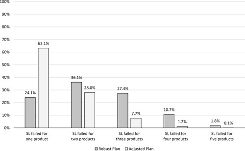
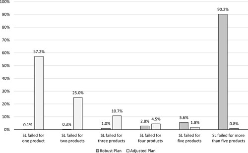
Figure 5. Detailed evaluation of PC 2 according to the number of products missing the target service level.

This bar chart visualizes for PC 2 the number of products missing the target service level, differentiated by violations for one, two, three, four, five or more than five products for both the robust and the adjusted plan.

For PC 1, as shown in Figure 4, in approximately 76% of infeasible replications, the target service level is violated for more than one product in the case of the robust and stable plan. The service level is mostly violated for two out of five products. This is the case in 36.1% of infeasible replications. In contrast, the service level is violated in the flexible approach in more than 63% of the infeasible replications for at most one product. In more than 90% of the infeasible replications, the service level is violated for only one or two products.

The results of PC 2, as illustrated in Figure 5, show even more clearly the advantage of flexible planning. The robust and stable plan fails to meet the target service level for more than five out of twenty products in more than 90% of infeasible replications. Only in 0.1% of infeasible replications, the target service level is violated for just one product. In contrast, the service level is violated in the flexible approach in more than 80% of the infeasible replications for at most two products. If there is a violation of the service level, the violation mostly affects only one out of twenty products (57.2% of infeasible replications). In more than 90% of the infeasible replications, the service level is violated for a maximum of three products.

5.2.2. Triangularly distributed proportion of defective products

We also performed a comparable simulation study for a triangularly distributed proportion of defective products. Here, we focussed on the test instances of PC 1. The results are shown in Table 8.

Table 8. Fraction of replications fulfilling the target service level for triangularly distributed proportion of defective products.

	Robust Plan	Adjusted Plan
SL	6.7%	52.7%
SL-0.1PP	60.1%	96.2%
SL-0.5PP	98.0%	∼100.0%
SL-1.0PP	∼100.0%	100.0%
SL-2.0PP	100.0%	100.0%
SL-3.0PP	100.0%	100.0%

The robust and stable plan fails to meet the target service level for more than 90% of the replications. In contrast, the flexible planning approach achieves the targeted service level for more than 50% of the replications. In this case, more than 90% of the replications miss the targeted service level by a maximum of 0.1 percentage points. As noted already by Helber, Sahling, and Schimmelpfeng (2013), our results demonstrate the high degree of flexibility of the scenario approach in the modelling of probabilistic dependencies.

As the results for the triangular distribution are quite similar to those of the uniform distribution, in the following, we focus on a uniformly distributed proportion of defective products.

5.3. Ex post analysis

In the next step, we perform an ex post analysis. In this analysis, we compared the objective function value after the last iteration of the multistage approach with the objective function value obtained by solving the deterministic CLSP-RW using the setup pattern determined in the first stage and knowing the proportion of defective products for each lot ex ante. Notably, only those replications of the test instances of both problem classes were considered for which the flexible planning approach violated the target service level by a maximum of 0.5 percentage points.

For a single TI, the deviation $\mathrm{De}{v}_{\mathrm{TI},r}^{\mathrm{Flex}}$ for each replication r can be calculated as follows: $\mathrm{De}{v}_{\mathrm{TI},r}^{\mathrm{Flex}}=\frac{Z_{\mathrm{TI},r}^{\mathrm{Flex}}-Z_{\mathrm{TI},r}^{\mathrm{ExPost}}}{Z_{\mathrm{TI},r}^{\mathrm{ExPost}}}$For each replication r of a single TI, the objective function value of the deterministic CLSP-RW is denoted by $Z_{\mathrm{TI},r}^{\mathrm{ExPost}}$, and the respective objective function value determined in the last iteration of the flexible planning approach is denoted by $Z_{\mathrm{TI},r}^{\mathrm{Flex}}$. The results of the ex post analysis are shown in Table 9.

Table 9. Results of ex post analysis.

	$\mathrm{ADe}{v}^{\mathrm{Flex}}$	$\mathrm{MDe}{v}^{\mathrm{Flex}}$
PC 1	0.19%	1.58%
PC 2	0.15%	0.70%

In columns $\mathrm{ADe}{v}^{\mathrm{Flex}}$ and $\mathrm{MDe}{v}^{\mathrm{Flex}}$, the average and maximum deviation are reported for both problem classes. With an average deviation of 0.19% in the case of PC 1 and 0.15% in the case of PC 2, the average deviation is very moderate. The maximum deviation of a replication is 1.58% for PC 1 and 0.70% for PC 2.

In addition, the replication with the highest deviation of 1.58% was analysed in more detail. For this TI, the optimal setup pattern was determined with ex ante knowledge of the exact proportion of defective items per lot. This can further improve the objective function value, as the setup pattern can be different from the robust setup pattern. However, the deviation increased only slightly to 2.1%. Thus, the results of the flexible planning approach are very close to the ex post solution.

5.4. Importance of flexible planning

We show the advantage of our flexible planning approach by comparing the resulting adjusted plan with a deterministic plan as well as with a robust and stable plan. For the deterministic production and rework plan, a variant of the CLSP-RW presented by Goerler and Voß (2016) was solved. Here, the CLSP-RW is extended by δ-service level constraints. According to Kang et al. (2017), we consider the case of an imperfect production process with a higher mean proportion of defective products ${\overline{\mathrm{\Omega }}}_k=0.1$ and a higher range ${\mathrm{Range}}_{\mathrm{\Omega }}=\pm 0.5\cdot {\overline{\mathrm{\Omega }}}_k$ of the uniformly distributed proportion of defective products.

For this part of our numerical study, we generated 24 new test instances for PC 1 by varying the remaining parameters according to Table 5. Furthermore, a comparable simulation study with 1,000 replications was conducted as presented in Subsection 5.2. The results are presented in Table 10.

Table 10. Comparison of deterministic, robust, and adjusted production and rework plans.

	Deterministic Plan	Robust Plan	Adjusted Plan
SL	2.3%	5.7%	61.8%
SL-0.1PP	3.6%	8.4%	80.9%
SL-0.5PP	14.0%	24.0%	96.8%
SL-1.0PP	37.1%	51.2%	100.0%
SL-2.0PP	83.8%	91.4%	100.0%
SL-3.0PP	98.9%	99.7%	100.0%

For the deterministic plan, more than 97% of the replications miss the target service level. In this case, more than 60% of the replications miss the target service level by more than one percentage point. The results of the robust production and rework plan are slightly better. More than 94% of the replications fail to meet the target service level. However, the flexible planning approach meets the service level in 61.8% of the replications. Notably, almost 97% of the replications of the flexible planning approach have a maximum violation of 0.5 percentage points.

The results show that our flexible planning approach performs very well even in the presence of a higher proportion of defective products and a higher variability. Furthermore, the adjusted production and rework plan significantly outperforms both the deterministic and robust plans.

5.5. Managerial insights

We now examine the effect of variability in the proportion of defective products on total costs. Therefor, we used four TIs derived from $\mathrm{PC}1$ with $\mathrm{K}=4$ products and $\mathrm{T}=6$ periods and a uniformly distributed proportion of defective products, as described in Table 11. For each TI, we first solved the SCLSP-RW${}^{\mathrm{SAA}}$ to optimality using CPLEX. Then, for each instance, we performed a simulation study, as described in Section 5.2, with 1,000 replications.

Table 11. Parameter setting.

Mean proportion of defective products	${\overline{\mathrm{\Omega }}}_k=0.1$
Range of the proportion of defective products	${\mathrm{Range}}_{\mathrm{\Omega }}\in \{\pm 0.1\cdot {\overline{\mathrm{\Omega }}}_k,\pm 0.5\cdot {\overline{\mathrm{\Omega }}}_k\}$
Variability of the demand	$V{C}_d=0.3$
Capacity utilisation	Util = 0.8
Time between orders	$\mathrm{TBO}\in \{1,4\}$
Target service level	$\delta =0.95$

In Figure 6, we report the objective function values of the robust production and rework plan for each TI. Note that the total cost is higher for a low TBO than it is for a high TBO. This can be explained by the determination of the holding cost $h{c}_k$ using (23(24) $\begin{array}{rl}{c}_t& =\frac{1}{\mathrm{Util}}\cdot \sum _{k\in \mathcal{K}}(p{t}_k\cdot {\overline{d}}_k+s{t}_k+p{t}_k^r\cdot {\overline{d}}_k\cdot {\overline{\mathrm{\Omega }}}_k+s{t}_k^r)\\ & \mathrm{\forall }t\in \mathcal{T}\end{array}$(24) ). According to Tempelmeier (2011), we keep the setup cost $s{c}_k$ constant for our test instances. Thus, a lower TBO results in higher holding cost $h{c}_k$. However, the relationship between setup and storage costs results in more frequent setup operations at a low TBO than at a high TBO.

Figure 6. Total expected costs of the robust production and rework plan.

This bar chart shows the impact of varying ranges of the proportion of defective products on the total expected costs of the robust production and rework plan in the case of low and high TBO.

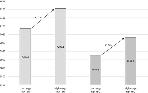
With increasing uncertainty, i.e. a larger range of the proportion of defective products, the objective function value increases. In addition, the increase in cost is slightly higher when the TBO is low.

The results of the simulation study are visualised in Figure 7. For each TI, we present the spread of the resulting total costs of the adjusted production and rework plan in a box plot diagram.

Figure 7. Spread of the total costs of the adjusted production and rework plan.

This box plot visualizes the impact of varying ranges of the proportion of defective products on the spread of total costs of the adjusted production and rework plan in the case of low and high TBO.

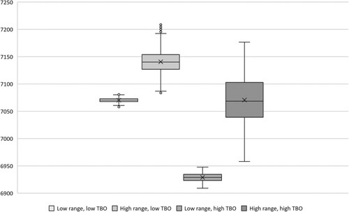
A higher variability in the proportion of defective products leads to a significantly higher variability in the total costs. In summary, actions to reduce the variability of the proportion of defective products (e.g. employee training) will reduce the expected costs. Furthermore, the described effect is stronger in production systems with lower setup costs compared to inventory holding costs (lower TBO), i.e. in the case of lean production. Considering the total costs of the adjusted production and rework plan, actions to reduce the variability of the proportion of defective products will also reduce the variability of the total costs. This effect is stronger in the case of a higher TBO.

6. Conclusion and outlook

This paper presents a novel approach to integrated production and rework planning with random proportion of defective products. The resulting nonlinear generic model formulation was linearised through a scenario-based approach. Our simulation-based analysis shows that the adjusted production and rework plans obtained by the proposed flexible planning approach significantly outperform both the deterministic and robust plans. Furthermore, an ex post analysis shows that the objective function values obtained under the application of the flexible planning approach and random proportion of defective products are close to those obtained under the assumption of complete knowledge of the proportion of defective products. Our managerial insights show that activities to reduce the variability of the proportion of defective products (e.g. employee training) are of greater importance in the case of lean production regarding the reduction of expected costs.

In the future, uncertain demand should be considered (see e.g. Helber, Sahling, and Schimmelpfeng 2013 or Hilger, Sahling, and Tempelmeier 2016). Moreover, in practice, rework times may depend on the severity of the failure of a particular defective item. Since the outcome of defective items is uncertain, the severity of defects that occur, and therefore the rework time required to fix defects, is also random. This results in a complex planning situation with stochastic proportion of defective products and stochastic rework times.

Acknowledgments

We would like to thank both anonymous reviewers for their careful reading of our manuscript. Their many insightful comments and suggestions helped to improve and clarify this manuscript. Results of this work were presented at the 14${}^{\mathrm{th}}$ International Workshop on Lot Sizing 2023 in Cork, Ireland. Furthermore, a few parts of this article were developed from Pierre Kohlmann's unpublished master thesis at the University of Kaiserslautern.

Data availability statement

The test instances of this study are available from the authors upon request.

Disclosure statement

No potential conflict of interest was reported by the author(s).

Correction Statement

This article has been corrected with minor changes. These changes do not impact the academic content of the article.

Additional information

Notes on contributors

Pierre Kohlmann

Pierre Kohlmann is a research assistant and doctoral student at the Chair of Production Management at the RPTU School of Business and Economics, University of Kaiserslautern-Landau, Germany. He received his M. Sc. in Business Management and Engineering from the University of Kaiserslautern, Germany. His research interests include lot sizing.

Florian Sahling

Florian Sahling holds the Chair of Production Management at the RPTU School of Business and Economics, University of Kaiserslautern-Landau, Germany. He holds a doctoral degree from Leibniz Universität Hannover, Germany. His main research interests are related to production planning and scheduling.

References

- Akçalı, E., and S. Çetinkaya. 2011. “Quantitative Models for Inventory and Production Planning in Closed-loop Supply Chains.” International Journal of Production Research 49 (8): 2373–2407. https://doi.org/10.1080/00207541003692021.
- Aloulou, M. A., A. Dolgui, and M. Y. Kovalyov. 2014. “A Bibliography of Non-deterministic Lot-sizing Models.” International Journal of Production Research 52 (8): 2293–2310. https://doi.org/10.1080/00207543.2013.855336.
- Asadkhani, J., H. Mokhtari, and S. Tahmasebpoor. 2022. “Optimal Lot-sizing Under Learning Effect in Inspection Errors with Different Types of Imperfect Quality Items.” Operational Research – An International Journal 22 (3): 2631–2665.
- Barzoki, M. R., M. Jahanbazi, and M. Bijari. 2011. “Effects of Imperfect Products on Lot Sizing with Work in Process Inventory.” Applied Mathematics and Computation 217 (21): 8328–8336. https://doi.org/10.1016/j.amc.2011.03.023.
- Biswas, P., and B. R. Sarker. 2008. “Optimal Batch Quantity Models for a Lean Production System with in-cycle Rework and Scrap.” International Journal of Production Research 46 (23): 6585–6610. https://doi.org/10.1080/00207540802230330.
- Bookbinder, J. H., and J. Y. Tan. 1988. “Strategies for the Probabilistic Lot-sizing Problem with Service-level Constraints.” Management Science 34 (9): 1096–1108. https://doi.org/10.1287/mnsc.34.9.1096.
- Brahimi, N, N. Absi, S. Dauzère-Pérès, and A. Nordli. 2017. “Single-item Dynamic Lot-sizing Problems: An Updated Survey.” European Journal of Operational Research 263 (3): 838–863. https://doi.org/10.1016/j.ejor.2017.05.008.
- Brahimi, N., S. Dauzère-Pérès, N. M. Najid, and A. Nordli. 2006. “Single Item Lot Sizing Problems.” European Journal of Operational Research 168 (1): 1–16. https://doi.org/10.1016/j.ejor.2004.01.054.
- Buschkühl, L., F. Sahling, S. Helber, and H. Tempelmeier. 2010. “Dynamic Capacitated Lot-sizing Problems: a Classification and Review of Solution Approaches.” OR Spectrum 32 (2): 231–261. https://doi.org/10.1007/s00291-008-0150-7.
- Cunha, J. O., H. H. Kramer, and R. A. Melo. 2019. “Effective Matheuristics for the Multi-item Capacitated Lot-sizing Problem with Remanufacturing.” Computers & Operations Research 104:149–158. https://doi.org/10.1016/j.cor.2018.12.012.
- Cunha, J. O., and R. A. Melo. 2016. “A Computational Comparison of Formulations for the Economic Lot-sizing with Remanufacturing.” Computers & Industrial Engineering 92:72–81. https://doi.org/10.1016/j.cie.2015.11.024.
- Devoto, C., E. Fernández, and P. Piñero. 2021. “The Economic Lot-sizing Problem with Remanufacturing and Inspection for Grading Heterogeneous Returns.” Journal of Remanufacturing 11 (1): 71–87. https://doi.org/10.1007/s13243-020-00089-5.
- Dolgui, A., M. Y. Kovalyov, and K. Shchamialiova. 2011. “Multi-product Lot-sizing and Sequencing on a Single Imperfect Machine.” Computational Optimization and Applications 50 (3): 465–482. https://doi.org/10.1007/s10589-010-9346-2.
- Fang, C., X. Liu, P. M. Pardalos, J. Long, J. Pei, and C. Zuo. 2017. “A Stochastic Production Planning Problem in Hybrid Manufacturing and Remanufacturing Systems with Resource Capacity Planning.” Journal of Global Optimization 68 (4): 851–878. https://doi.org/10.1007/s10898-017-0500-6.
- Flapper, S. D. P., J. C. Fransoo, R. A. C. M. Broekmeulen, and K. Inderfurth. 2002. “Planning and Control of Rework in the Process Industries: a Review.” Production Planning & Control 13 (1): 26–34. https://doi.org/10.1080/09537280110061548.
- Florian, M., J. K. Lenstra, and A. H. G. R. Kan. 1980. “Deterministic Production Planning: Algorithms and Complexity.” Management Science 26 (7): 669–679. https://doi.org/10.1287/mnsc.26.7.669.
- Giglio, D., M. Paolucci, and A. Roshani. 2017. “Integrated Lot Sizing and Energy-efficient Job Shop Scheduling Problem in Manufacturing/remanufacturing Systems.” Journal of Cleaner Production 148:624–641. https://doi.org/10.1016/j.jclepro.2017.01.166.
- Goerler, A., E. Lalla-Ruiz, and S. Voß. 2020. “Late Acceptance Hill-climbing Matheuristic for the General Lot Sizing and Scheduling Problem with Rich Constraints.” Algorithms 13 (6): 138. https://doi.org/10.3390/a13060138.
- Goerler, A., and S. Voß. 2016. “Dynamic Lot-sizing with Rework of Defective Items and Minimum Lot-size Constraints.” International Journal of Production Research 54 (8): 2284–2297. https://doi.org/10.1080/00207543.2015.1070970.
- Haojie, Y., M. Lixin, and Z. Canrong. 2017. “Capacitated Lot-Sizing Problem with One-way Substitution: A Robust Optimization Approach.” In 2017 3rd International Conference on Information Management (ICIM), Chengdu, China, 159–163. https://doi.org/10.1109/INFOMAN.2017.7950367.
- Harris, F. W. 1913. “How Many Parts to Make At Once.” Factory, The Magazine of Management 10 (2): 135–136, 152. Reprint in: Operations Research (1990), 38(6), 947–950
- Helber, S., K. Inderfurth, F. Sahling, and K. Schimmelpfeng. 2018. “Flexible Versus Robust Lot-scheduling Subject to Random Yield and Deterministic Dynamic Demand.” IISE Transactions 50 (3): 217–229. https://doi.org/10.1080/24725854.2017.1357089.
- Helber, S., and F. Sahling. 2010. “A Fix-and-optimize Approach for the Multi-level Capacitated Lot Sizing Problem.” International Journal of Production Economics 123 (2): 247–256. https://doi.org/10.1016/j.ijpe.2009.08.022.
- Helber, S., F. Sahling, and K. Schimmelpfeng. 2013. “Dynamic Capacitated Lot Sizing with Random Demand and Dynamic Safety Stocks.” OR Spectrum 35 (1): 75–105. https://doi.org/10.1007/s00291-012-0283-6.
- Hilger, T., F. Sahling, and H. Tempelmeier. 2016. “Capacitated Dynamic Production and Remanufacturing Planning Under Demand and Return Uncertainty.” OR Spectrum 38 (4): 849–876. https://doi.org/10.1007/s00291-016-0441-3.
- Inderfurth, K., G. Lindner, and N. P. Rachaniotis. 2005. “Lot Sizing in a Production System with Rework and Product Deterioration.” International Journal of Production Research 43 (7): 1355–1374. https://doi.org/10.1080/0020754042000298539.
- Jamal, A. M. M., B. R. Sarker, and S. Mondal. 2004. “Optimal Manufacturing Batch Size with Rework Process At a Single-stage Production System.” Computers & Industrial Engineering 47 (1): 77–89. https://doi.org/10.1016/j.cie.2004.03.001.
- Kang, C. W., M. Ullah, B. Sarkar, I. Hussain, and R. Akhtar. 2017. “Impact of Random Defective Rate on Lot Size Focusing Work-in-process Inventory in Manufacturing System.” International Journal of Production Research 55 (6): 1748–1766. https://doi.org/10.1080/00207543.2016.1235295.
- Kang, C. W., M. Ullah, M. Sarkar, M. Omair, and B. Sarkar. 2019. “A Single-stage Manufacturing Model with Imperfect Items, Inspections, Rework, and Planned Backorders.” Mathematics 7 (5): 446. https://doi.org/10.3390/math7050446.
- Karimi, B., S. M. T. Fatemi Ghomi, and J. M. Wilson. 2003. “The Capacitated Lot Sizing Problem: a Review of Models and Algorithms.” Omega 31 (5): 365–378. https://doi.org/10.1016/S0305-0483(03)00059-8.
- Kirste, M. 2017. Dynamic Lot Sizing Problems with Stochastic Production Output. Norderstedt: Books on Demand.
- Kleywegt, A. J., A Shapiro, and T. Homem-de-Melo. 2002. “The Sample Average Approximation Method for Stochastic Discrete Optimization.” SIAM Journal on Optimization 12 (2): 479–502. https://doi.org/10.1137/S1052623499363220.
- Lay, G., C. Dreher, and S. Kinkel. 1996. “Neue Produktionskonzepte leisten einen Beitrag zur Sicherung des Standorts Deutschland.” Positiver Zusammenhang zwischen der Verwirklichung neuer Konzepte und der Steigerung betrieblicher Leistungskennziffern belegt. Bulletins ‘German Manufacturing Survey’ (1), Fraunhofer Institute for Systems and Innovation Research (ISI).
- Levitan, R. E. 1960. “The Optimum Reject Allowance Problem.” Management Science 6 (2): 172–186. https://doi.org/10.1287/mnsc.6.2.172.
- Li, Y., J. Chen, and X. Cai. 2007. “Heuristic Genetic Algorithm for Capacitated Production Planning Problems with Batch Processing and Remanufacturing.” International Journal of Production Economics 105 (2): 301–317. https://doi.org/10.1016/j.ijpe.2004.11.017.
- Llewellyn, R. W. 1959. “Order Sizes for Job Lot Manufacturing.” Journal of Industrial Engineering 10 (3): 176–180.
- Pan, Z., J. Tang, and O. Liu. 2009. “Capacitated Dynamic Lot Sizing Problems in Closed-loop Supply Chain.” European Journal of Operational Research 198 (3): 810–821. https://doi.org/10.1016/j.ejor.2008.10.018.
- Pflug, G. C., and A. Pichler. 2014. Multistage Stochastic Optimization. Heidelberg: Springer Cham.
- Retel Helmrich, M. J., R. Jans, W. van den Heuvel, and A. P. M. Wagelmans. 2014. “Economic Lot-sizing with Remanufacturing: Complexity and Efficient Formulations.” IIE Transactions 46 (1): 67–86. https://doi.org/10.1080/0740817X.2013.802842.
- Roshani, A., M. Paolucci, D. Giglio, M. Demartini, F. Tonelli, and M. A. Dulebenets. 2023. “The Capacitated Lot-sizing and Energy Efficient Single Machine Scheduling Problem with Sequence Dependent Setup Times and Costs in a Closed-loop Supply Chain Network.” Annals of Operations Research 321 (1–2): 469–505. https://doi.org/10.1007/s10479-022-04783-4.
- Rudert, S., and U. Buscher. 2022. “Heuristics for the Single-Item Dynamic Lot-Sizing Problem with Rework of Internal Returns.” In Computational Logistics, ICCL 2022. Vol. 13557 of Lecture Notes in Computer Science, edited by J. de Armas, H. Ramalhinho, and S. Voß, 425–440. Barcelona: Springer Cham.
- Sahling, F. 2010. Mehrstufige Losgrößenplanung Bei Kapazitätsrestriktionen. Wiesbaden: Gabler Verlag. https://doi.org/10.1007/978-3-8349-8708-2.
- Sahling, F. 2013. “A Column-Generation Approach for a Short-Term Production Planning Problem in Closed-Loop Supply Chains.” BuR – Business Research 6 (1): 55–75. https://doi.org/10.1007/BF03342742.
- Sahling, F. 2016. “Integration of Vendor Selection Into Production and Remanufacturing Planning Subject to Emission Constraints.” International Journal of Production Research 54 (13): 3822–3836. https://doi.org/10.1080/00207543.2016.1148276.
- Saliby, E. 1990. “Descriptive Sampling: a Better Approach to Monte Carlo Simulation.” Journal of the Operational Research Society 41 (12): 1133–1142. https://doi.org/10.1057/jors.1990.180.
- Sarkar, B., L. E. Cárdenas-Barrón, M. Sarkar, and M. L. Singgih. 2014. “An Economic Production Quantity Model with Random Defective Rate, Rework Process and Backorders for a Single Stage Production System.” Journal of Manufacturing Systems 33 (3): 423–435. https://doi.org/10.1016/j.jmsy.2014.02.001.
- Schulz, T. 2011. “A New Silver-Meal Based Heuristic for the Single-item Dynamic Lot Sizing Problem with Returns and Remanufacturing.” International Journal of Production Research 49 (9): 2519–2533. https://doi.org/10.1080/00207543.2010.532916.
- Suzanne, E., N. Absi, and V. Borodin. 2020. “Towards Circular Economy in Production Planning: Challenges and Opportunities.” European Journal of Operational Research 287 (1): 168–190. https://doi.org/10.1016/j.ejor.2020.04.043.
- Syed Ali, S. A., M. Doostmohammadi, K. Akartunalı, and R. van der Meer. 2018. “A Theoretical and Computational Analysis of Lot-sizing in Remanufacturing with Separate Setups.” International Journal of Production Economics 203:276–285. https://doi.org/10.1016/j.ijpe.2018.07.002.
- Taleizadeh, A. A., L. E. Cárdenas-Barrón, and B. Mohammadi. 2014. “A Deterministic Multi Product Single Machine EPQ Model with Backordering, Scraped Products, Rework and Interruption in Manufacturing Process.” International Journal of Production Economics 150:9–27. https://doi.org/10.1016/j.ijpe.2013.11.023.
- Tempelmeier, H. 2011. “A Column Generation Heuristic for Dynamic Capacitated Lot Sizing with Random Demand Under a Fill Rate Constraint.” Omega 39 (6): 627–633. https://doi.org/10.1016/j.omega.2011.01.003.
- Tempelmeier, H. 2013. “Stochastic Lot Sizing Problems.” In Handbook of Stochastic Models and Analysis of Manufacturing System Operations. Vol. 192 of International Series in Operations Research & Management Science, edited by J. M. Smith, B. Tan, 313–344. New York, NY: Springer.
- Teunter, R. H., Z. P. Bayindir, and W. van den Heuvel. 2006. “Dynamic Lot Sizing with Product Returns and Remanufacturing.” International Journal of Production Research 44 (20): 4377–4400. https://doi.org/10.1080/00207540600693564.
- van Zyl, A., and O. Adetunji. 2022. “A Lot Sizing Model for Two Items with Imperfect Manufacturing Process, Time Varying Demand and Return Rates, Dependent Demand and Different Quality Grades.” Journal of Remanufacturing 12 (2): 227–252. https://doi.org/10.1007/s13243-022-00110-z.
- Vladimirou, H., and S. A. Zenios. 1997. “Stochastic Programming and Robust Optimization.” In Advances in Sensitivity Analysis and Parametric Programming. Vol. 6. of International Series in Operations Research & Management Science, edited by T. Gal, H. J. Greenberg, 395–447. Boston, MA: Springer.
- Widyana, G. A., and H. M. Wee. 2012. “An Economic Production Quantity Model for Deteriorating Items with Multiple Production Setups and Rework.” International Journal of Production Economics 138 (1): 62–67. https://doi.org/10.1016/j.ijpe.2012.02.025.
- Zhang, Z.-H., H. Jiang, and X. Pan. 2012. “A Lagrangian Relaxation Based Approach for the Capacitated Lot Sizing Problem in Closed-loop Supply Chain.” International Journal of Production Economics 140 (1): 249–255. https://doi.org/10.1016/j.ijpe.2012.01.018.
- Zhang, J., X. Liu, and Y. L. Tu. 2011. “A Capacitated Production Planning Problem for Closed-loop Supply Chain with Remanufacturing.” The International Journal of Advanced Manufacturing Technology 54 (5–8): 757–766. https://doi.org/10.1007/s00170-010-2948-0.
- Zouadi, T., A. Yalaoui, and M. Reghioui. 2018. “Hybrid Manufacturing/remanufacturing Lot-sizing and Supplier Selection with Returns, Under Carbon Emission Constraint.” International Journal of Production Research 56 (3): 1233–1248. https://doi.org/10.1080/00207543.2017.1412524.