Existence and properties of the logarithmic layer in oscillating flows

Abstract

The existence and properties of the logarithmic layer in a turbulent streamwise oscillating flow are investigated through direct numerical simulations and wall-resolved large-eddy simulations. The phase dependence of the von Kármán constant and the logarithmic layer intercept is explored for different values of the Reynolds number and the depth-ratio between the water depth and the Stokes boundary layer thickness. The logarithmic layer exists for a longer fraction of the oscillating period and a larger fraction of the water depth with increasing values of the Reynolds number. However, the values of both the von Kármán and the intercept depend on the phase, the Reynolds number and depth-ratio. Additionally, the simulations characterized by a low value of the depth-ratio and Reynolds number show intermittent existence of the logarithmic layer. Finally, the Reynolds number based on the friction velocity does not support a previously mentioned analogy between oscillatory flows and steady wall-bounded flows.

Keywords:

• Boundary layer turbulence
• direct numerical simulations
• large eddy simulations
• logarithmic layer
• oscillatory flows
• von Kármán constant

1. Introduction

Turbulent boundary layers are of interest in many engineering fields such as hydraulic engineering and coastal engineering. As a result, turbulent boundary layers are often subject to studies based on large-scale and high Reynolds number simulations. However, such flows are generally computationally expensive to fully resolve numerically (Piomelli & Balaras, 2002; Radhakrishnan & Piomelli, 2008). Sufficient resolution is required in the wall normal direction to resolve the boundary layer. Additionally, sufficient resolution is also important for resolving the separation of scales between the large-scale energy carrying eddies and the small-scale dissipative eddies. As a result, these difficulties are often bypassed using a so called wall-model, in which the flow velocity close to the wall are parametrized (Piomelli & Balaras, 2002; Radhakrishnan & Piomelli, 2008). Although different wall models exist, the most commonly used is based on the “law of the wall” (Marusic et al., 2010; Piomelli & Balaras, 2002; Radhakrishnan & Piomelli, 2008), a classical theory for wall-bounded flows and described below.

In classical wall-bounded flow theory, it is assumed that the velocity distribution in a wall-bounded flow can be categorized in four regions or layers (Nieuwstadt, Boersma, & Westerweel, 2016; Radhakrishnan & Piomelli, 2008). Starting at the wall, there is, first, the viscous sub-layer, where the flow is dominated by viscous forces and where the non-dimensional velocity $u^{\mathtt{+}}=⟨u⟩/u_{\tau }$ varies linearly with the non-dimensional height $y^{\mathtt{+}}=y{u}_{\tau }/\nu$ according to $u^{\mathtt{+}}=y^{\mathtt{+}}$. In these formulae, $⟨u⟩$ is the ensemble averaged mean velocity in the streamwise direction, $u_{\tau }=\sqrt{{\tau }_w/\rho }=\sqrt{\nu (\mathrm{\partial }⟨u⟩/\mathrm{\partial }y{)}_w}$ is the friction velocity, y is the height above the wall, ${\tau }_w$ is the wall shear stress, ρ is the fluid density, and ν is the kinematic viscosity. Second, there is the buffer layer, where the viscous model is not valid any more and no simple scaling for the velocity exists. The buffer layer is connecting the viscous sub-layer to the third layer, the logarithmic layer. In the logarithmic layer (in this manuscript also referred to as log-layer or log-region), the velocity is logarithmically dependent on $y^{\mathtt{+}}$ according to: (1) $u^{\mathtt{+}}=\frac{1}{\kappa }\ln \left(y^{\mathtt{+}}\right)+B$(1) with κ the von Kármán constant and B the logarithmic layer intercept. Finally, there is the outer layer, for which a theoretical expression depending on the type of flow is also possible, but will not be considered here (e.g. Kundu & Cohen, 2002).

In most models relying on the law of the wall, the first computational point is assumed to be located within the log-layer (Piomelli & Balaras, 2002). The suitability of these models is now widely accepted. First, it is possible to derive the log-layer analytically, based on scaling arguments (Nieuwstadt et al., 2016), and second, the existence of the log-layer has been observed for steady flows in many studies, including numerical simulations (Hoyas & Jiménez, 2006; Jiménez & Moser, 2007; Kim, Moin, & Moser, 1987), experiments (Marusic, Monty, Hultmark, & Smits, 2013; Mckeon, Li, Jiang, Morrison, & Smits, 2004; Perry & Li, 1990) and field measurements (Andreas et al., 2006; Frenzen & Vogel, 1995). Moreover, a log-region has also been detected in streamwise oscillating flows (Akhavan, Kamm, & Shapiro, 1991; Hsu, Lu, & Kwan, 2000; Jensen Sumer, & Fredsøe, 1989; Jonsson & Carlsen, 1976; Salon, Armenio, & Crise, 2007; Scandura, Faraci, & Foti, 2016; Tuzi & Blondeaux, 2008) even if its theoretical derivation ignores the mean local acceleration (Nieuwstadt et al., 2016; Piomelli & Balaras, 2002). It is important to note that the log-layer was also studied in spanwise oscillating flows. Under spanwise wall oscillations, the transient behaviour of the boundary layer when adjusting itself to a lower drag state has implications for the log-region (Skote, 2014).

In an early study, Jonsson (1980) developed a phase-dependent expression linking the velocity to the logarithm of the depth. However, this model was already assuming the existence of a logarithmic layer. Although Sleath (1987) found that this theoretical expression agreed well with his measurements, he also admitted that equally good agreement could be obtained for several different values of the von Kármán constant. Additionally, the expression was based on rough wall flows, and Mujal-Colilles, Christensen, Bateman, and Garcia (2016) showed that rough walls generated different coherent structures than smooth walls, at least in the transition to turbulence. Radhakrishnan and Piomelli (2008) obtained good agreement between numerical simulations of a streamwise oscillating flow and experimental data at high Reynolds numbers, while using a law-of-the-wall as boundary condition. They used a hybrid wall model composed of a viscous sub-layer part (in which the velocity scales linearly with depth), and a log-layer part, in order to take into account low Reynolds number effects when the wall shear stress changes sign. Indeed, several studies have shown that a log-region does not necessarily exist at all times in flows for which the mean properties are highly time dependent (Hino, Kashiwayanagi, Nakayama, & Hara, 1983; Jensen et al., 1989; Salon et al., 2007). For example, Jensen et al. (1989) found that for a steamwise oscillating flow there can be large parts of the oscillation cycle where no logarithmic layer is detected, with its presence interval depending strongly on the value of the Reynolds number. As a result, the existence of the log-layer and its properties need to be thoroughly investigated. Using these properties, the conditions for which it is justified to use a wall model in turbulent non-steady flows can be defined.

In this manuscript, we present the results of an analysis of the existence and the properties of the logarithmic layer in a canonical unsteady flow: the turbulent oscillating boundary layer. Besides being a classical example of a statistically time-dependent flow, the turbulent oscillating boundary layer has many applications, for example, in biology (e.g. pulmonary flows; see Tuzi & Blondeaux, 2008) and in coastal engineering (e.g. tidal channel flows; see Gross & Nowell, 1983; Li, Sanford, & Chao, 2005). Additionally, the existence and properties of the log-region are crucial in many computer model applications where the boundary layer cannot be resolved. These properties need to be known, and this is the purpose of the present study. Our study is based on results of direct numerical simulations (DNS) and large eddy simulations (LES) of an open channel flow driven by a homogeneous, uniform, streamwise, oscillating pressure gradient: (2) $-\frac{1}{\rho }\frac{\mathrm{\partial }P}{\mathrm{\partial }x}=U_0\omega \cos \left(\omega t\right)$(2) with P the pressure, x the coordinate in the streamwise direction, $U_0$ the amplitude of the free-stream velocity, ω the angular frequency and t the time. The flow is characterized by two non-dimensional parameters: the Reynolds number based on the thickness of the Stokes boundary layer ${\mathsf{R}}_{\delta }\mathsf{=}{\mathsf{U}}_{\mathsf{0}}{\delta }_{\mathsf{s}}\mathsf{/}\nu$, characterizing the transition to turbulence (Jensen et al., 1989; Salon et al., 2007), and the ratio between the water depth h and the Stokes boundary layer thickness ${\delta }_s$ (for definitions, see Section 2). Different configurations are simulated, covering different applications, e.g. high value of ${\mathsf{R}}_{\delta }$ and a relatively low value of $h/{\delta }_s$ for simulations of tidal-like boundary layers, or low value of ${\mathsf{R}}_{\delta }$ and large value of $h/{\delta }_s$ for simulations of wave-like boundary layers. As a result, for the first time, the logarithmic layer is characterized as a function of ${\mathsf{R}}_{\delta }$ , $h/{\delta }_s$ and the phase of the oscillating pressure gradient.

2. Problem formulation

The flow is governed by the non-dimensional equations for conservation of mass and momentum of an incompressible flow and a homogeneous fluid: (3a) $\begin{array}{rl}\frac{\mathrm{\partial }{\overline{u}}_i^{\ast }}{\mathrm{\partial }{x}_i^{\ast }}& =0\end{array}$(3a) (3b) $\begin{array}{rl}\frac{\mathrm{\partial }{\overline{u}}_i^{\ast }}{\mathrm{\partial }{t}^{\ast }}+{\overline{u}}_j^{\ast }\frac{\mathrm{\partial }{\overline{u}}_i^{\ast }}{\mathrm{\partial }{x}_j^{\ast }}& =-\frac{\mathrm{\partial }{\overline{p}}^{\ast }}{\mathrm{\partial }{x}_i^{\ast }}+\frac{1}{{\mathsf{R}}_{\delta }}\frac{{\delta }_s}{h}\frac{{\mathrm{\partial }}^2{\overline{u}}_i^{\ast }}{\mathrm{\partial }{x}_j^{\ast 2}}\\ & +\frac{2}{{\mathsf{R}}_{\delta }}\frac{h}{{\delta }_s}\cos \left(\frac{2}{{\mathsf{R}}_{\delta }}\frac{h}{{\delta }_s}{t}^{\ast }\right){\delta }_{i1}-\frac{\mathrm{\partial }{\tau }_{ij}^{\ast }}{\mathrm{\partial }{x}_j^{\ast }}\end{array}$(3b) The symbol $\overline{\cdot }$ denotes a filtered quantity; ${\overline{u}}_i^{\ast }=({\overline{u}}^{\ast },{\overline{v}}^{\ast },{\overline{w}}^{\ast })$ is the non-dimensional filtered velocity in the non-dimensional $x_i^{\ast }$ direction (i.e. streamwise $\left(x^{\ast }\right)$, vertical $\left(y^{\ast }\right)$ and spanwise $\left(z^{\ast }\right)$); $t^{\ast }$ is the non-dimensional time; ${\overline{p}}^{\ast }$ is the non-dimensional pressure; ${\delta }_{i1}$ is the Kronecker delta, and ${\tau }_{ij}^{\ast }$ is the contribution of the subgrid-scale stresses to the flow field. These stresses are either equal to zero (in DNS configuration) or modelled using the dynamic Smagorinsky approach (in LES configuration); see Scotti and Piomelli (2001), Salon et al. (2007) and Armenio and Piomelli (2000). Additionally, the i subscript refers to a spatial direction while the j subscript refers to an implicit summation over the three directions. The velocities are scaled with $U_0$, the time with $h/U_0$, the spatial dimensions with h and the pressure with $\rho U_0^2$. The second term on the right hand side of Eq. (3b(3b) $\begin{array}{rl}\frac{\mathrm{\partial }{\overline{u}}_i^{\ast }}{\mathrm{\partial }{t}^{\ast }}+{\overline{u}}_j^{\ast }\frac{\mathrm{\partial }{\overline{u}}_i^{\ast }}{\mathrm{\partial }{x}_j^{\ast }}& =-\frac{\mathrm{\partial }{\overline{p}}^{\ast }}{\mathrm{\partial }{x}_i^{\ast }}+\frac{1}{{\mathsf{R}}_{\delta }}\frac{{\delta }_s}{h}\frac{{\mathrm{\partial }}^2{\overline{u}}_i^{\ast }}{\mathrm{\partial }{x}_j^{\ast 2}}\\ & +\frac{2}{{\mathsf{R}}_{\delta }}\frac{h}{{\delta }_s}\cos \left(\frac{2}{{\mathsf{R}}_{\delta }}\frac{h}{{\delta }_s}{t}^{\ast }\right){\delta }_{i1}-\frac{\mathrm{\partial }{\tau }_{ij}^{\ast }}{\mathrm{\partial }{x}_j^{\ast }}\end{array}$(3b) ) represents the viscous stresses, while the third term is a homogeneous large-scale pressure gradient $\mathrm{\partial }{P}^{\ast }/\mathrm{\partial }{x}^{\ast }$ driving the flow, such that: (4) $-\frac{\mathrm{\partial }{P}^{\ast }}{\mathrm{\partial }{x}^{\ast }}=\frac{2}{{\mathsf{R}}_{\delta }}\frac{h}{{\delta }_s}\cos \left(\frac{2}{{\mathsf{R}}_{\delta }}\frac{h}{{\delta }_s}{t}^{\ast }\right)$(4) The two previously discussed non-dimensional quantities (${\mathsf{R}}_{\delta }$ and $h/{\delta }_s$) appear in the equations, where the thickness of the Stokes boundary layer is defined as: (5) ${\delta }_s=\sqrt{\frac{2\nu }{\omega }}$(5) and the Reynolds number as: (6) ${\mathsf{R}}_{\delta }\mathsf{=}\frac{{\mathsf{U}}_{\mathsf{0}}{\delta }_{\mathsf{s}}}{\nu }$(6) If $h/{\delta }_s$ is large enough, ${\mathsf{R}}_{\delta }$ is the only parameter governing the transition to turbulence (Jensen et al., 1989; Kaptein, Duran-Matute, Roman, Armenio, & Clercx, 2019; Salon et al., 2007). Here, large enough means that the turbulent boundary layer is not influenced by the water-depth, which is the case for $h/{\delta }_s\ge 25$ for ${\mathsf{R}}_{\delta }\le \mathsf{1790}$ or $h/{\delta }_s\ge 40$ for $1790\le {\mathsf{R}}_{\delta }\le \mathsf{3460}$ (Kaptein et al., 2019). The simulated values of the Reynolds number are ${\mathsf{R}}_{\delta }\mathsf{=}\mathsf{990}\mathsf{,}\mathsf{1790}$ and 3460, and for each Reynolds number, five different $h/{\delta }_s$ ratios are considered: $h/{\delta }_s=5,10,25,40$ and 70. Previous studies (Jensen et al., 1989; Kaptein et al., 2019) show that the flow is in the intermittent turbulent regime for ${\mathsf{R}}_{\delta }\mathsf{=}\mathsf{990}$ and in the fully turbulent regime for ${\mathsf{R}}_{\delta }\mathsf{=}\mathsf{1790}$ and ${\mathsf{R}}_{\delta }\mathsf{=}\mathsf{3460}$, although fully developed turbulence is not observed through the entire oscillation cycle. Additionally, damping of turbulence is observed during part of the cycle for $h/{\delta }_s\le 10$ and throughout the entire cycle for $h/{\delta }_s\le 5$, for these three values of the Reynolds number (Kaptein et al., 2019). Equations (3a(3a) $\begin{array}{rl}\frac{\mathrm{\partial }{\overline{u}}_i^{\ast }}{\mathrm{\partial }{x}_i^{\ast }}& =0\end{array}$(3a) ) and (3b(3b) $\begin{array}{rl}\frac{\mathrm{\partial }{\overline{u}}_i^{\ast }}{\mathrm{\partial }{t}^{\ast }}+{\overline{u}}_j^{\ast }\frac{\mathrm{\partial }{\overline{u}}_i^{\ast }}{\mathrm{\partial }{x}_j^{\ast }}& =-\frac{\mathrm{\partial }{\overline{p}}^{\ast }}{\mathrm{\partial }{x}_i^{\ast }}+\frac{1}{{\mathsf{R}}_{\delta }}\frac{{\delta }_s}{h}\frac{{\mathrm{\partial }}^2{\overline{u}}_i^{\ast }}{\mathrm{\partial }{x}_j^{\ast 2}}\\ & +\frac{2}{{\mathsf{R}}_{\delta }}\frac{h}{{\delta }_s}\cos \left(\frac{2}{{\mathsf{R}}_{\delta }}\frac{h}{{\delta }_s}{t}^{\ast }\right){\delta }_{i1}-\frac{\mathrm{\partial }{\tau }_{ij}^{\ast }}{\mathrm{\partial }{x}_j^{\ast }}\end{array}$(3b) ) are integrated numerically using a fractional step finite-difference method, based on the algorithm of Zhang, Street, and Khoseff (1994). For more details see Salon et al. (2007) and Salon, Armenio, and Crise (2009). The size of the computational domain is $65{\delta }_s$ in the streamwise direction and $32{\delta }_s$ in the spanwise direction, except for the simulation with $h/{\delta }_s=5$ and ${\mathsf{R}}_{\delta }\mathsf{=}\mathsf{1790}$ (characterized by a high level of intermittency) where the domain size is doubled in each horizontal direction. The domain size is overall in agreement with the size of the turbulent structures (Costamagna, Vittori, & Blondeaux, 2003; Jiménez & Moin, 1991), and the horizontal boundary conditions are periodic. At the bottom boundary, a no-slip condition is applied, and at the top boundary, a no-stress condition is applied. A sketch of the domain is provided in Fig. 1, alongside the velocity profiles for the analytical solution of the laminar flow.

Figure 1. Sketch of the computational domain. The red profiles represent the analytical solution of the laminar oscillating flow at four different phases $\omega t=0$, $\pi /2$, π and $3\pi /2$. The analytical solution is given by $u(y,t)=-U_0\exp \left(\omega t\right)\sin (\omega t-y/{\delta }_s)+U_0\sin \left(\omega t\right)$ for $u_0=1$ and ${\delta }_s=1$

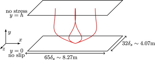
The simulations with ${\mathsf{R}}_{\delta }\mathsf{=}\mathsf{990}$ are performed with DNS, and the simulations with ${\mathsf{R}}_{\delta }\mathsf{=}\mathsf{1790}$ and ${\mathsf{R}}_{\delta }\mathsf{=}\mathsf{3460}$ are performed with LES. The number of grid cells in the vertical varies from 64 for the simulation ${\mathsf{R}}_{\delta }\mathsf{=}\mathsf{990}$ and $h/{\delta }_s=5$ to 640 for the simulations with ${\mathsf{R}}_{\delta }\mathsf{=}\mathsf{3460}$ and $h/{\delta }_s=70$. The cells are clustered close to the bottom boundary such that the first grid point is at $y^{\mathtt{+}}=1$. The value of $y^{\mathtt{+}}$ used for grid considerations is defined with respect to the maximum of ${\tau }_w$ over the oscillation cycle, implying $y^{\mathtt{+}}=1$ is a “worst case scenario”. For most of the oscillation cycle, the first grid point is located at $y^{\mathtt{+}}<1$. In both DNS and LES configuration, there are at least five points (without counting the bottom boundary itself) located in the viscous sub-layer and part of the buffer layer, i.e. $y^{\mathtt{+}}\le 11$. In the horizontal directions, 256 grid points are used for ${\mathsf{R}}_{\delta }\mathsf{=}\mathsf{990}$ (DNS configuration), 128 grid points are used for ${\mathsf{R}}_{\delta }\mathsf{=}\mathsf{1790}$ (LES configuration), and 192 grid points are used for ${\mathsf{R}}_{\delta }\mathsf{=}\mathsf{3460}$ (LES configuration). As mentioned by Kaptein et al. (2019), the horizontal resolution in wall units varies from less than $45y^{+}$ in LES configuration to $12y^{+}$ in DNS configuration. The spanwise grid spacing varies from at most $22y^{+}$ for the LES simulations to $14y^{+}$ in DNS configuration. The validation of the software package is extensively described by Salon et al. (2007) while the validation of the present dataset is described by Kaptein et al. (2019). The wall shear stress and the velocity profiles have been compared to experimental data of Jensen et al. (1989), and a good agreement was found. Additionally, for two of the simulations with $h/{\delta }_s\le 10$ and ${\mathsf{R}}_{\delta }\le \mathsf{1790}$, grid convergence was checked and obtained by doubling the vertical or the horizontal resolution. For the particular case with $h/{\delta }_{s=5}$ and ${\mathsf{R}}_{\delta }\mathsf{=}\mathsf{1790}$, convergence was only obtained after reducing the value of the Courant number from 0.6 to 0.3. For $h/{\delta }_s=5$ and ${\mathsf{R}}_{\delta }\mathsf{=}\mathsf{990}$, grid convergence could not be obtained. An overview of the simulation settings is given in Table 1.

Table 1. Numerical settings for each simulation

${\mathsf{R}}_{\delta }$	$h/{\delta }_s$	$n_x^a$	$n_y^a$	$n_z^a$	$L_x/{\delta }_s^a$	$L_z/{\delta }_s^a$	Technique
990	5	512	64	512	130	64	DNS
990	10	256	80	256	65	32	DNS
990	25	256	144	256	65	32	DNS
990	40	256	208	256	65	32	DNS
990	70	256	352	256	65	32	DNS
1790	5	256	80	256	130	64	LES
1790	10	128	112	128	65	32	LES
1790	25	128	176	128	65	32	LES
1790	40	128	256	128	65	32	LES
1790	70	128	376	128	65	32	LES
3460	5	192	96	192	65	32	LES
3460	10	192	144	192	65	32	LES
3460	25	192	304	192	65	32	LES
3460	40	192	480	192	65	32	LES
3460	70	192	640	192	65	32	LES

${}^{\mathrm{a}}$ The symbols $n_x$, $n_y$ and $n_z$ are the number of grid cells in the streamwise, vertical and spanwise directions. The symbols $L_x$ and $L_z$ are the domain size in the streamwise and spanwise direction.

The velocity field is saved every phase interval $\mathrm{\Delta }\omega t=\pi /12$ for about 20 periods. Velocity profiles and other statistics are obtained by plane-averaging, and when possible, phase-averaging of the velocity fields. The possibility of performing phase-averaging depends on the nature of the flow. If a flow is intermittent for a specific phase, phase averaging would combine laminar velocity fields and turbulent velocity fields, which is not desirable.

3. Results

3.1. Identification of the logarithmic layer

The determination of the existence and the extent of the logarithmic layer is a well-known challenge in the study of turbulent flows (Hoyas & Jiménez, 2006; Marusic et al., 2013). The logarithmic depth dependence of the streamwise velocity is based on the assumption that the turbulence eddies scale with the distance from the wall (Townsend, 1961); a hypothesis that has been frequently debated and that seems only satisfied at very high values of the Reynolds number (Perry & Li, 1990). As a result, the velocity profile slightly deviates from the logarithmic asymptote, even in the so-called logarithmic region (Bernardini, Pirozzoli, & Orlandi, 2014). This is the log-layer defect and makes the log-layer more challenging to detect (Marusic et al., 2013).

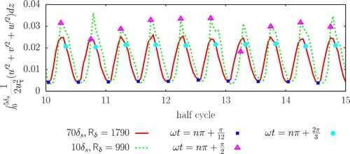
An additional challenge is that some of the present simulations are characterized by intermittent turbulence. The intermittent character of the flow is visualized for two simulations in Fig. 2, by means of the resolved turbulent kinetic energy (TKE), integrated over a $5{\delta }_s$ thick layer close to the wall. Identical phases are marked by a symbol, and the position of these symbols demonstrates that the TKE is nearly constant from cycle to cycle for ${\mathsf{R}}_{\delta }\mathsf{=}\mathsf{1790}$, $h/{\delta }_s=70$ and $\omega t=\pi /12$ (low value of the TKE) and $\omega t=2\pi /3$ (high value of the TKE). However, for ${\mathsf{R}}_{\delta }\mathsf{=}\mathsf{990}$, $h/{\delta }_s=10$ and $\omega t=\pi /2$ the TKE strongly varies from cycle to cycle indicating intermittency for these parameter settings.

Figure 2. Resolved TKE within a $5{\delta }_s$ thick layer adjacent to the bottom boundary layer for 10 successive half cycles. The two curves represent simulations with different values of the Reynolds number and the $h/{\delta }_s$ ratio. The symbols mark the TKE values at specific phases

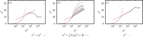
The impact of this intermittency on the velocity profiles can be seen in Fig. 3, in which the plane-averaged velocity profiles have been plotted for three different value combinations of ${\mathsf{R}}_{\delta }\mathsf{,}\mathsf{h}\mathsf{/}{\delta }_{\mathsf{s}}$ and the phase of the surface velocity (denoted $\omega t$). The profiles have not yet been phase-averaged, which means that each value combination leads to about 20 profiles, each of them corresponding to a distinct oscillation cycle. The sub-figures of Fig. 3 clearly show three different regimes. In Fig. 3a, none of the profiles for the parameter values ${\mathsf{R}}_{\delta }\mathsf{=}\mathsf{1790}$, $h/{\delta }_s=70$ and $\omega t=\pi /12$ approaches the theoretical log-law curve given by Eq. (1(1) $u^{\mathtt{+}}=\frac{1}{\kappa }\ln \left(y^{\mathtt{+}}\right)+B$(1) ): this is the non-logarithmic regime. In Fig. 3b, some of the profiles for ${\mathsf{R}}_{\delta }\mathsf{=}\mathsf{990}$, $h/{\delta }_s=10$ and $\omega t=\pi /2$ do approach this log-law while others are still a long way from it: this is the intermittent regime. Finally, in Fig. 3c all the profiles for ${\mathsf{R}}_{\delta }\mathsf{=}\mathsf{1790}$, $h/{\delta }_s=70$ and $\omega t=2\pi /3$ collapse on the log law: this is the logarithmic regime. The results of Fig. 3 reveal two important findings. First, the log-layer is not necessarily present for all values of $\omega t$, at given ${\mathsf{R}}_{\delta }$ and $h/{\delta }_s$. Second, still at given ${\mathsf{R}}_{\delta }$ and $h/{\delta }_s$, there might be some phases where the presence of the log-layer for a certain $\omega t$ also depends on the specific oscillation cycle. This latter finding is particularly important when computing the values of κ and B. The accuracy of these values is related to the size of statistical sample from which they are computed, such that phase-averaging is needed for improved precision. However, it only makes sense to average profiles that have a log-layer. As a result, conditional averaging will be performed, and phases with no well-defined log-layer will be excluded. Under the assumption that a log-layer is a signature of the turbulent character of a flow, the conditional averaging can be regarded as averaging exclusively over the turbulent flow fields.

Figure 3. Profiles of the plane-averaged, streamwise non-dimensional velocity $u^{\mathtt{+}}$ in semi-logarithmic scale for three different value combination of ${\mathsf{R}}_{\delta }$, $h/{\delta }_s$ and $\omega t$. (a) ${\mathsf{R}}_{\delta }\mathsf{=}\mathsf{1790}$, $h/{\delta }_s=70$ and $\omega t=\pi /12$, (b) ${\mathsf{R}}_{\delta }\mathsf{=}\mathsf{990}$, $h/{\delta }_s=10$ and $\omega t=\pi /2$, and (c) ${\mathsf{R}}_{\delta }\mathsf{=}\mathsf{1790}$, $h/{\delta }_s=70$ and $\omega t=2\pi /3$. The theoretical solution has been obtained for $\kappa =0.41$ and B=5.5

As a result, the plane-averaged velocity profiles with a logarithmic layer had to be identified by eye for all values of the parameters ${\mathsf{R}}_{\delta }$, $h/{\delta }_s$ and $\omega t$. This identification is obviously quite subjective, and had to be performed for about $12\times 2\times 20\times 5\times 3=7200$ profiles. The number 12 refers to the number of phases considered, 2 to the symmetry of the oscillation cycle, 20 to the number of oscillation cycles, 3 to the number of different values for ${\mathsf{R}}_{\delta }$ and 5 to the number of different values for $h/{\delta }_s$.

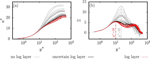
To gain more confidence and objectivity in our estimations, but also to avoid repeating the subjective identification procedure in the future, we want to find a robust signature of the log-layer in the simulation data. It has been suggested in previous work (Afzal & Yajnik, 1973; Bernardini et al., 2014; Jiménez & Moser, 2007; Pirozzoli, Bernardini, & Orlandi, 2014) that a good method to analyse velocity profiles could be done through the log-law diagnostic function Ξ defined as: (7) $\mathrm{\Xi }=\frac{\mathrm{d}{u}^{\mathtt{+}}}{\mathrm{d}\ln \left(y^{\mathtt{+}}\right)}=y^{\mathtt{+}}\frac{\mathrm{d}{u}^{\mathtt{+}}}{\mathrm{d}{y}^{\mathtt{+}}}$(7) This quantity is supposed to reach a plateau equal to $1/\kappa$ (the inverse of the von Kármán constant) in the log-region but several studies (Hoyas & Jiménez, 2006; Jiménez & Moser, 2007) report that such a flat region is never reached. This finding suggest that the log-law diagnostic function is not more suitable for detecting the log-layer than the velocity profile. However, Fig. 4 shows that Ξ still gives valuable information. In Fig. 4a, the velocity profiles of Fig. 3b (in the intermittent regime) are reproduced, while differentiating the profiles that are logarithmic (red-dashed), the profiles that are not logarithmic (grey-solid), and the profiles for which the presence of the log-layer is uncertain (black-solid). These three profile categories are then investigated in terms of Ξ (Fig. 4b), and one specific feature emerges concerning the height in wall units at which Ξ is locally maximum. This height is larger than the thickness of the viscous sub-layer (located at $y^{\mathtt{+}}=5$) but smaller than the centre of the buffer layer (located at $y^{\mathtt{+}}=17$). As a result, we will call this height the “thickness of the viscosity dominated layer”: a layer where the molecular viscosity is dominant but turbulent fluctuation are not necessarily negligible. The advantage of this definition is that it can be used for laminar, turbulent and intermittent flows. The thickness of the viscosity dominated layer seems to be constant and approximately equal to $y^{\mathtt{+}}=10$, when the profile approaches the log-layer, but it increases significantly up to values of approximately $y^{\mathtt{+}}=22$, when the flow does not have a log-layer. This evolution in the location of the local maximum has been earlier observed by Hino et al. (1983).

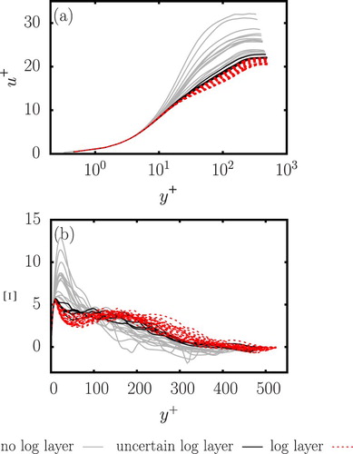
Figure 4. (a) Reproduction of the profiles of Fig. 3 while differentiating the profiles having a log-layer (red-dashed) from the ones that did not have a log-layer (grey-solid) and the ones for which the presence of the log-layer is uncertain (black-solid) and (b) their associated log-layer diagnostic function Ξ for ${\mathsf{R}}_{\delta }\mathsf{=}\mathsf{990}$, $h/{\delta }_s=10$ and $\omega t=\pi /2$. The absence of a plateau at $1/\kappa$ for Ξ might be difficult to detect in logarithmic scale. Therefore, this figure has been reproduced in normal scaling in the Appendix, Fig. 13

Taking advantage of this trend, two maps of points defined by the coordinates $(\ln (y_{vs}^{\mathtt{+}});⟨u(y_{vs}^{\mathtt{+}})⟩/U_0)$ are displayed in Fig. 5, with $y_{vs}^{\mathtt{+}}$ the height of the first local maximum of Ξ and $⟨u\left(y_{vs}^{\mathtt{+}}\right)⟩/U_0$ the value of the velocity at that height. Figure 5a contains points from all the simulations with ${\mathsf{R}}_{\delta }\mathsf{=}\mathsf{990}$ while Fig. 5b contains points from all the simulations with ${\mathsf{R}}_{\delta }\mathsf{=}\mathsf{3460}$. Each point represents $(\ln (y_{vs}^{\mathtt{+}});⟨u(y_{vs}^{\mathtt{+}}/U_0)⟩)$ for a given phase $\omega t$ in an oscillation cycle for one of the simulations. The points in each panel form a distinct shape with three branches: (i) a first branch drawing a convex path from the bottom left corner to the top right corner of the figure, (ii) a second branch going from the top right corner to the centre of the figure and (iii) a third branch going from the centre of the figure towards the bottom. The first and second branches coincide with points from the laminar analytical solution of Stokes' second problem displayed in blue (e.g. Kaptein et al., 2019), while the third branch approaches the theoretical line $y_{vs}^{\mathtt{+}}=11$ displayed with a black dashed line. This line results from the assumption that the thickness of the viscosity dominated layer can be obtained by equating the scaling function in the viscous sub-layer, i.e. $u^{\mathtt{+}}=y^{\mathtt{+}}$, and the scaling function in the logarithmic layer, i.e. Eq. (1(1) $u^{\mathtt{+}}=\frac{1}{\kappa }\ln \left(y^{\mathtt{+}}\right)+B$(1) ). Forcing the intersection of these two lines at $y^{\mathtt{+}}=11$ gives B=5.2 for $\kappa =0.41$.

Figure 5. Points of coordinates $(\ln (y_{vs}^{\mathtt{+}});⟨u(y_{vs}^{\mathtt{+}})⟩/U_0)$, i.e. the height of the viscous sub-layer and its associated velocity. Each point corresponds to a specific value of the phase $\omega t$, a specific period and a specific value of $h/{\delta }_s$. (a) ${\mathsf{R}}_{\delta }\mathsf{=}\mathsf{990}$ and (b) ${\mathsf{R}}_{\delta }\mathsf{=}\mathsf{3460}$. The plane-averaged velocity $⟨u⟩$ has been made non-dimensional with the outer scale $U_0$ instead of the inner scale $u_{\tau }$ because in this way the difference between the laminar points and the turbulent points is emphasized. The points of the laminar solution are obtained by taking the first maximum of $y^{\mathtt{+}}\mathrm{\partial }{u}_{\mathrm{\infty }}/\mathrm{\partial }y$, where $u_{\mathrm{\infty }}$ is the analytical solution under infinite depth assumption (Kaptein et al., 2019). The start of the oscillating cycle $\omega t=0$ is marked by the blue circle

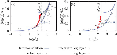
The symbols in Figs 5a and b follow the same trend. At the beginning of the oscillation cycle (denoted by the blue circle), the light grey diamonds are distributed close to the curve of the laminar solution. The profiles are in the non-logarithmic regime. As the oscillation cycle progresses, the grey diamond follow the blue curve towards the top-right until they reach the phase at which transition to turbulence occurs. This phase is highly dependent on the value of ${\mathsf{R}}_{\delta }$ (Jensen et al., 1989). When the flow transitions to turbulence, the grey diamonds leave the laminar curve and migrate towards the line defined by $y_{vs}^{\mathtt{+}}=11$. When approaching this line, the profiles enter the logarithmic regime, marked by the red points. In the logarithmic regime, the red points follow approximately the line $y_{vs}^{\mathtt{+}}=11$, until they reach again the blue line of the laminar solution. This joining happens at the end of the deceleration phase, just before a new boundary layer builds up in the other direction, and might indicate that the presence of the log-layer at theses phases is due to a history effect rather than equilibrium turbulence.

Although the symbols in Figs 5a and b describe similar paths, there are also discrepancies. First, it can be seen that the logarithmic branch in Fig. 5b is closer to the theoretical line $y_{vs}^{\mathtt{+}}=11$ than the logarithmic branch in panel 5a, but it still deviates from it. These differences already suggest that the constants κ and B probably depend on both ${\mathsf{R}}_{\delta }$ and the phase $\omega t$. Second, some of the light grey diamonds in Fig. 5a are located outside the branches, on the right of the non-logarithmic branch; these points are from the shallowest simulations, i.e. with $h/{\delta }_s=5$ and $h/{\delta }_s=10$. These simulations are characterized by such a high level of intermittency that the symmetry in the oscillation cycle is broken leading to a net flow in one direction over an oscillation cycle. This phenomenon is not explicitly shown or discussed here but has also been observed by Tuzi and Blondeaux (2008) and might explain the out-of-trend location of these points, particularly because for higher Reynolds number values, all points collapse into the curves (Fig. 5b).

The free-stream phases particularly characterized by intermittency are summarized in Table 2. Intermittent turbulence is restricted to a few phases in simulations with either a low value of ${\mathsf{R}}_{\delta }$ or a low value of $h/{\delta }_s$. The intermittency will be taken into account while computing the ensemble-averaged statistics, i.e. we are considering in these cases conditional phase-averaged vertical profiles of streamwise velocity. From now on, these profiles will be both plane and phase averaged. For the phases characterized by intermittency, only the velocity fields in which the presence of the logarithmic layer is confirmed by diagrams as shown in Fig. 5 are used in the phase averaging. As mentioned previously, discarding flow fields with no log-layer comes down to using only turbulent flow fields for computing the properties of the log-layer.

Table 2. Overview of the phases characterized by intermittency. These phases are defined as the profiles for which, at identical value of ${\mathsf{R}}_{\delta }$, $h/{\delta }_s$ and $\omega t$, the $(\ln (y_{vs}^{\mathtt{+}});⟨u(y_{vs}^{\mathtt{+}})⟩/U_0)$ points are located simultaneously on the logarithmic branch and significantly off the logarithmic edge

${\mathsf{R}}_{\delta }$	$h/{\delta }_s$	$\omega t$
990	5	$\frac{7}{12}\pi ,\frac{2}{3}\pi ,\frac{3}{4}\pi ,\frac{5}{6}\pi$
990	10	$\frac{1}{2}\pi ,\frac{7}{12}\pi$
990	25, 40, 70	$\frac{5}{12}\pi$
1790	5	$\frac{5}{12}\pi ,\frac{1}{2}\pi ,\frac{7}{12}\pi$
3460	5	$\frac{1}{12}\pi$

3.2. Von Kármán constant and intercept

Even if the velocity profile is characterized by the presence of a logarithmic region, we anticipated that the characteristics of this region will depend on the value of the governing parameters and on the phase. Here, we obtain the values of the von Kármán constant κ and the intercept B used in the logarithmic fit given by Eq. (1(1) $u^{\mathtt{+}}=\frac{1}{\kappa }\ln \left(y^{\mathtt{+}}\right)+B$(1) ). Although it is possible to find κ and B by fitting Eq. (1(1) $u^{\mathtt{+}}=\frac{1}{\kappa }\ln \left(y^{\mathtt{+}}\right)+B$(1) ) through the log region, we prefer to determine the constant and the intercept in a different way. In fact, the fitting procedure requires that initially the extent of the log region is subjectively determined, and this should be done for all the plane- and phase-averaged velocity profiles (up to 180 profiles). Instead, we propose a simpler procedure that is easier to reproduce. We first assume the necessary but not sufficient condition that the logarithmic region can only exist for $y_{\mathrm{m}\mathrm{i}\mathrm{n}}^{\mathtt{+}}<y^{\mathtt{+}}<y_{\mathrm{m}\mathrm{a}\mathrm{x}}^{\mathtt{+}}$. The depth $y_{\mathrm{m}\mathrm{i}\mathrm{n}}^{\mathtt{+}}$ is then defined as the thickness of the viscosity dominated layer (which was computed in the previous section), i.e. $y_{\mathrm{m}\mathrm{i}\mathrm{n}}^{\mathtt{+}}=y_{vs}^{\mathtt{+}}$. The depth $y_{\mathrm{m}\mathrm{a}\mathrm{x}}^{\mathtt{+}}$ is in turn defined as the depth $y^{\mathtt{+}}$ at which $⟨u⟩$ reaches its first local maximum. In this way, $y_{\mathrm{m}\mathrm{a}\mathrm{x}}^{\mathtt{+}}$ can be interpreted as the thickness of the boundary layer, depending on the phase $\omega t$. For $y_{\mathrm{m}\mathrm{i}\mathrm{n}}^{\mathtt{+}}<y^{\mathtt{+}}<y_{\mathrm{m}\mathrm{a}\mathrm{x}}^{\mathtt{+}}$, we then determine the depth $y_c^{\mathtt{+}}$ at which Ξ is minimum and call this depth $y_c^{\mathtt{+}}$ the centre of the logarithmic layer. The introduced $y_{\mathrm{m}\mathrm{i}\mathrm{n}}^{\mathtt{+}}$ and $y_c^{\mathtt{+}}$ are sketched in Fig. 6a while $y_{\mathrm{m}\mathrm{a}\mathrm{x}}^{\mathtt{+}}$ is sketched in Fig. 6b. The value of the von Kármán constant is then $\kappa =1/\mathrm{\Xi }\left(y_c^{\mathtt{+}}\right)$, and the value of the intercept is $B=u^{\mathtt{+}}\left(y_c^{\mathtt{+}}\right)-\ln \left(y_c^{\mathtt{+}}\right)/\kappa$.

Figure 6. Sketch of (a) a velocity profile in logarithmic scale with its corresponding log-layer diagnostic function for ${\mathsf{R}}_{\delta }\mathsf{=}\mathsf{990}$, $h/{\delta }_s=10$ and $\omega t=\pi /2$ and (b) a velocity profile for ${\mathsf{R}}_{\delta }\mathsf{=}\mathsf{3460}$, $h/{\delta }_s=70$ and $\omega t=\pi /2$. The thickness of the viscous sub-layer $y_{\mathrm{m}\mathrm{i}\mathrm{n}}\equiv y_{vs}^{\mathtt{+}}$ and $y_c$ are sketched on (a) while $y_{\mathrm{m}\mathrm{a}\mathrm{x}}^{\mathtt{+}}$ is sketched on (b)

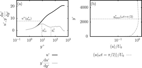
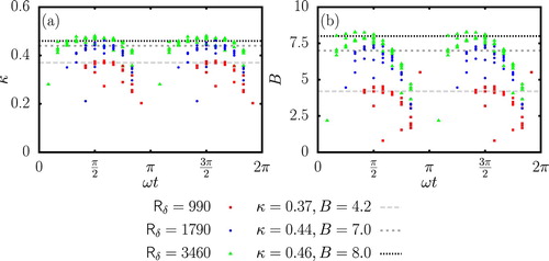
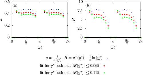
Figure 7 displays κ and B as a function of the phase for each value of ${\mathsf{R}}_{\delta }$ and $h/{\delta }_s$. It can be seen, that the average values of κ and B depend strongly on the value of ${\mathsf{R}}_{\delta }$. The mean von Kármán constant κ increases from 0.37 at ${\mathsf{R}}_{\delta }\mathsf{=}\mathsf{990}$ to 0.46 at ${\mathsf{R}}_{\delta }\mathsf{=}\mathsf{3460}$, which is slightly different from the values obtained by Tuzi and Blondeaux (2008) in a pipe flow simulation. For ${\mathsf{R}}_{\delta }\mathsf{=}\mathsf{8000}$ and $R/{\delta }_s=4$ (with R the radius of their pipe), they found a von Kármán constant of 0.4 and an intercept at 5.5. Note that $R/{\delta }_s$ is similar to $h/{\delta }_s$ except that R is also a measure of the curvature of the bottom boundary, while the bottom boundary in the open channel configuration is flat. Similarly, the mean value of B increases from 4.2 at ${\mathsf{R}}_{\delta }\mathsf{=}\mathsf{990}$ to 8.0 at ${\mathsf{R}}_{\delta }\mathsf{=}\mathsf{3460}$. The dependence of κ on the Reynolds number was already observed by Frenzen and Vogel (1995) and Nagib and Chauhan (2008) for steady flows. However, in those cases, κ decreases with increasing value of the Reynolds number. Additionally, Marusic et al. (2010) stated that the value of κ depends on the type of wall-bounded flow (e.g. pipe flow or channel flow), which might explain the small discrepancies between our results and the results from Tuzi and Blondeaux (2008). A last feature is the decrease of both κ and B at the end of the deceleration phase (around $\omega t=\pi$), with a much stronger decrease for B than for κ. This decrease is remarkable as it is not observed at the beginning of the acceleration phase (i.e. in the presence of a favourable pressure gradient), suggesting an asymmetry between the acceleration and the deceleration phases (i.e. in the presence of an adverse pressure gradient). The asymmetry reinforces an assumption mentioned earlier: the observed log-layer is not related to the turbulence conditions at this particular phase, but to the remainder of a log-layer that had been generated in an earlier stage of the flow. Finally, similarly to the points in Fig. 5, some points are out-of-trend and these points again correspond to simulations with $h/{\delta }_s=5$, making the presence of a true logarithmic region at these values of $h/{\delta }_s$ questionable.

Figure 7. Evolution of the von Kármán constant (a) and the intercept B (b) as a function of the phase $\omega t$. The influence of the Reynolds number has been highlighted by using different coloured symbols for the data points corresponding to simulations with different values of ${\mathsf{R}}_{\delta }$. All values of $h/{\delta }_s$ are considered. Different dotted lines are also displayed in order to indicate specific values of κ and B

The established values and observed trends for κ and B are critically based on their definitions, i.e. $\kappa =1/\mathrm{\Xi }\left(y_c^{\mathtt{+}}\right)$ and $B=u^{\mathtt{+}}\left(y_c^{\mathtt{+}}\right)-\ln \left(y_c^{\mathtt{+}}\right)/\kappa$. To test the sensitivity of the results to these definitions, κ and B have also been estimated via a linear fit in Fig. 8. The fitting interval was chosen such that the relative error $E$ satisfies: (8) $E\left(y^{\mathtt{+}}\right)=\left|\frac{\frac{1}{\kappa }\ln \left(y^{\mathtt{+}}\right)+B-u^{\mathtt{+}}\left(y^{\mathtt{+}}\right)}{u^{\mathtt{+}}\left(y^{\mathtt{+}}\right)}\right|\le \epsilon$(8) with ϵ maximum value of the error. The new values of κ and B for ${\mathsf{R}}_{\delta }\mathsf{=}\mathsf{3460}$ and $h/{\delta }_s=40$ are displayed in Fig. 8a and b, respectively. On one side, it is obvious from this figure that the previously mentioned discrepancies between the observed values of κ and B in the present study, and the values in the literature, can be attributed to the way of computing them. In fact, when the fitting method is used, the von Kármán constant becomes extremely close to 0.41 for $\epsilon =0.065$. Similarly, the value of B is then also lower with respect to the method using $\kappa =1/\mathrm{\Xi }\left(y_c^{\mathtt{+}}\right)$ and $B=u^{\mathtt{+}}\left(y_c^{\mathtt{+}}\right)-\ln \left(y_c^{\mathtt{+}}\right)/\kappa$. For higher values of $\epsilon =0.115$, κ and B decrease further. This result proves that the method used to determine these constants is crucial for the accuracy of the results.

Figure 8. Value of the von Kármán constant (a) and the intercept B (b) as a function of the phase $\omega t$, for ${\mathsf{R}}_{\delta }\mathsf{=}\mathsf{3460}$ and $h/{\delta }_s=40$. Two different ways of computing κ and B are tested. One is based on the minimum of the log-layer diagnostic function Ξ (blue dots) and the other is based on fitting a function through an interval depending on the relative error Err of the velocity profile with respect to the log-law (red triangles and green diamonds)

On the other side the general trend in the phase-evolution of κ and B is observed throughout the oscillation cycle, except for the earlier phases. The reduction in κ and B at the end of the deceleration phases is still observed and supports once more that the log-layer presence at these phases is due to a history effect. In contrast, the different behaviour of κ and B at $\omega t=\pi /6$ and $\pi /4$ could imply that the formation process of the log-layer is not yet completed at these phases.

3.3. Spatial and temporal extent of the logarithmic layer

The determination of the spatial extent of the log-layer is something quite subjective too (Hoyas & Jiménez, 2006; Marusic et al., 2013). In Section 3.2 we mentioned the necessary condition that the log-layer could only exist for $y_{\mathrm{m}\mathrm{i}\mathrm{n}}^{\mathtt{+}}<y^{\mathtt{+}}<y_{\mathrm{m}\mathrm{a}\mathrm{x}}^{\mathtt{+}}$. However, the spatial extent could also be smaller than $[y_{\mathrm{m}\mathrm{i}\mathrm{n}}^{\mathtt{+}}:y_{\mathrm{m}\mathrm{a}\mathrm{x}}^{\mathtt{+}}]$, such that this condition is not sufficient. Here, we assume that the spatial extent of the log-layer is the space-interval at which the relative error, $E$, defined in Eq. (8(8) $E\left(y^{\mathtt{+}}\right)=\left|\frac{\frac{1}{\kappa }\ln \left(y^{\mathtt{+}}\right)+B-u^{\mathtt{+}}\left(y^{\mathtt{+}}\right)}{u^{\mathtt{+}}\left(y^{\mathtt{+}}\right)}\right|\le \epsilon$(8) ), is smaller than $\epsilon =5\cdot {10}^{-3}$. The coefficients used in Eq. (8(8) $E\left(y^{\mathtt{+}}\right)=\left|\frac{\frac{1}{\kappa }\ln \left(y^{\mathtt{+}}\right)+B-u^{\mathtt{+}}\left(y^{\mathtt{+}}\right)}{u^{\mathtt{+}}\left(y^{\mathtt{+}}\right)}\right|\le \epsilon$(8) ) are computed using the method proposed in this paper, $\kappa =1/\mathrm{\Xi }\left(y_c^{\mathtt{+}}\right)$ and $B=u^{\mathtt{+}}\left(y_c^{\mathtt{+}}\right)-\ln \left(y_c^{\mathtt{+}}\right)/\kappa$. The start and the end of the log-layer for each ratio $h/{\delta }_s$ and each ${\mathsf{R}}_{\delta }$ according to this definition are plotted as a function of the phase in Fig. 9. For all the simulations, the log-layer starts around $25<y^{\mathtt{+}}<50$ (in agreement with the literature results of Tennekes & Lumley, 1972) but extends over different lengths, mainly depending on the value of ${\mathsf{R}}_{\delta }$. Clearly, the spatial extent of the log-layer increases with the value of the Reynolds number, although these increments are less significant between ${\mathsf{R}}_{\delta }\mathsf{=}\mathsf{1790}$ and ${\mathsf{R}}_{\delta }\mathsf{=}\mathsf{3460}$ than between ${\mathsf{R}}_{\delta }\mathsf{=}\mathsf{990}$ and ${\mathsf{R}}_{\delta }\mathsf{=}\mathsf{1790}$. In general, the water depth does not seem to affect the spatial extent except for ${\mathsf{R}}_{\delta }\mathsf{=}\mathsf{1790}$ and $h/{\delta }_s=5$ where it drastically increases when compared to the other values of $h/{\delta }_s$. At $\omega t=\pi /2$, the log-region extends up to $y^{\mathtt{+}}=300$ while the surface is located at $y^{\mathtt{+}}=414$. This difference is relatively small, particularly considering the small value of ϵ that is used to define the spatial extent. The proximity of the end of the log-layer and the surface could suggests an interaction between the logarithmic layer and the top boundary. The choice of the boundary condition plays an important role in this situation. In a lot of environmental applications, a free-surface boundary conditions is more realistic. The free-surface would probably lead to more complex interactions with the log-layer. However, it also introduces an additional parameter, the Froude number. The incorporation of a free-surface would make the isolation of the Reynolds number effects or reduced water-depth effect more difficult and is not in the scope of the present study. Finally, peaks in the spatial extent of the log-layer are observed at the earliest phases where the log-layer is detected. These peaks might be related to the formation process of the log-layer already discussed earlier, still ongoing at these phases, making its detection and extent more sensitive to the setting of ϵ or to the evaluation of the characteristic point defined by $(\ln (y_{vs}^{\mathtt{+}}),⟨u(y_{vs}^{\mathtt{+}})⟩/U_0)$. This phenomenon also explains why a log-layer is detected at $\omega t=\pi /5$ for ${\mathsf{R}}_{\delta }\mathsf{=}\mathsf{1790}$ and $h/{\delta }_s=40$ but not for the other values of $h/{\delta }_s$ at ${\mathsf{R}}_{\delta }\mathsf{=}\mathsf{1790}$.

Figure 9. Spatial extent and existence interval of the log-layer, depending on ${\mathsf{R}}_{\delta }$ and $h/{\delta }_s$: ${\mathsf{R}}_{\delta }\mathsf{=}\mathsf{990}$ (a), ${\mathsf{R}}_{\delta }\mathsf{=}\mathsf{1790}$ (b) and ${\mathsf{R}}_{\delta }\mathsf{=}\mathsf{3460}$ (c). The open symbols and dashed line mark the start for the logarithmic region and the filled symbols and solid line mark its end

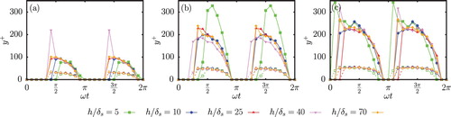
Similarly to the spatial extent, the phase interval during which the log-layer is present (the presence interval) also increases with the value of the Reynolds number. The size of the presence interval also appears to be related to the ratio $h/{\delta }_s$. For ${\mathsf{R}}_{\delta }\mathsf{=}\mathsf{3460}$ and $h/{\delta }_s=5$, the presence interval of the log-layer is shifted by a phase $\mathrm{\Delta }\omega t=\pi /12$ towards the earlier phases, but the size of the presence interval remains approximately the same compared to the higher $h/{\delta }_s$ values. For lower ${\mathsf{R}}_{\delta }$ values, the influence of the reduction of the water-depth is more significant as the size of the presence interval reduces. For ${\mathsf{R}}_{\delta }\mathsf{=}\mathsf{990}$, the presence interval reduces with decreasing $h/{\delta }_s$ from $\pi /3\le \omega t\le 11\pi /12$ at $h/{\delta }_s=10$ to $5\pi /12\le \omega t\le \pi$ at $h/{\delta }_s=5$. For ${\mathsf{R}}_{\delta }\mathsf{=}\mathsf{1790}$, the size of presence interval reduces from $\pi /4\le \omega t\le 11\pi /12$ at $h/{\delta }_s=10$ to $\pi /3\le \omega t\le 5\pi /12$, implying that this size reduction increases with decreasing value of ${\mathsf{R}}_{\delta }$.

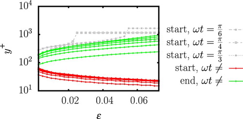
The findings about the spatial-extent and time-interval presence of the log-layer have been obtained for a specific value of ϵ. To understand how the spatial-extent changes for a different value of ϵ, the start and the end of the log-layer are plotted as function of ϵ in Fig. 10, for ${\mathsf{R}}_{\delta }\mathsf{=}\mathsf{3460}$, $h/{\delta }_s=40$. Each line represents the start (or end) of the log-layer at different phase $\omega t$. For $\omega t\in \{\pi /6;\pi /4;\pi /3\}$, the end of the log-layer reaches a plateau for a certain value of ϵ. This plateau is equal to $y_{\mathrm{m}\mathrm{a}\mathrm{x}}^{\mathtt{+}}$ and implies that the log-layer has reached its maximum extent. For the other values of $\omega t$, the end of the log-layer increases and the start of the log-layer decreases uniformly with ϵ, conserving the relative extent observed for $\epsilon =5\cdot {10}^{-3}$.

Figure 10. Start and end of the log-layer depending on the maximum error ϵ for ${\mathsf{R}}_{\delta }\mathsf{=}\mathsf{3460}$, $h/{\delta }_s=40$. Each green line or red line marks a different value of the phase $\omega t$

3.4. Reynolds number based on the friction velocity

So far, this study shows that the presence of the logarithmic layer in turbulent oscillating flows depends on three different parameters ${\mathsf{R}}_{\delta }$, $h/{\delta }_s$ and $\omega t$. Nevertheless, previous research demonstrate that, when fully developed turbulence is observed in the oscillating flow, the behaviour of the flow is nearly identical to that of a steady wall-bounded flow (Jensen et al., 1989; Salon et al., 2007). In these steady boundary layer flows, the existence and properties of the log-layer are usually investigated in term of one single parameter: ${\mathsf{R}}_{}$, the Reynolds number based on the friction velocity $u_{\tau }$: (9) ${\mathsf{R}}_{}\mathsf{=}\frac{{\mathsf{u}}_{\tau }\mathsf{d}}{\nu }$(9) where d is the channel half depth. As an example, Kim et al. (1987) detected a log-layer in their velocity profile for ${\mathsf{R}}_{}\mathsf{=}\mathsf{180}$ in their pioneering DNS study of a steady plane channel flow. The definition of a characteristic parameter for unsteady turbulent flows was already discussed for pulsating flows (Ramaprian & Tu, 1983; Scotti & Piomelli, 2001). It was proposed to use the eddy viscosity to define a turbulent Stokes layer thickness as a characteristic length scale rather than Eq. (5(5) ${\delta }_s=\sqrt{\frac{2\nu }{\omega }}$(5) ). However, although the eddy viscosity could be computed directly from the simulations, its depth dependence implies that a unique value of the eddy viscosity per phase does not exist.

Instead of using the turbulent Stokes layer thickness, we investigate the possibility of extending the use of ${\mathsf{R}}_{}$ to an oscillating flow, to analyse the standard approach used to study logarithmic layers in steady flows, and to test its validity for non-steady flows. This extension makes use of a different interpretation of d. In a turbulent plane channel flow, d is also the largest distance that a fluid parcel can be separated from the closest wall, such that d is a measure of the thickness of the wall-dominated layer. As a result, the velocity at a distance d of the wall is the maximum velocity in the water column. The analogy with the turbulent oscillating boundary layer is then quickly made: d should be defined as the height at which the velocity profile has its (first) maximum. In fact, $u_{\tau }d/\nu =y_{\mathrm{m}\mathrm{a}\mathrm{x}}^{\mathtt{+}}$, such that $u_{\tau }d/\nu$ has already been sketched in Fig. 6b for ${\mathsf{R}}_{}\mathsf{=}\mathsf{3460}$ and $h/{\delta }_s=70$.

A first advantage of using ${\mathsf{R}}_{}$ is that d and $u_{\tau }$, and therefore ${\mathsf{R}}_{}$, depend on $\omega t$. Additionally, a previous study on the same dataset (Kaptein et al., 2019) determined that ${\mathsf{R}}_{\delta }$ is the only parameter governing the flow as long as d<h throughout the oscillation cycle, but that $h/{\delta }_s$ has to be taken into account if d=h during at least part of cycle. 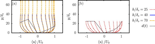A second advantage of using ${\mathsf{R}}_{}$ is that it takes into account this specific $h/{\delta }_s$ dependence. In Fig. 11a, h>d, and it can be seen that both d and $u_{\tau }$ are identical for $h/{\delta }_s=40$ and $h/{\delta }_s=70$ at fixed phase $\omega t$, and for ${\mathsf{R}}_{\delta }\mathsf{=}\mathsf{3460}$. This similarity implies that ${\mathsf{R}}_{\delta }$ is also identical for $h/{\delta }_s=40$ and $h/{\delta }_s=70$ at this specific Reynolds number. In Fig. 11b, $h\ngtr d$ for some part of the oscillation cycle, such that d and eventually $u_{\tau }$ are different between $h/{\delta }_s=25$ and $h/{\delta }_s=70$ for ${\mathsf{R}}_{\delta }\mathsf{=}\mathsf{3460}$. These differences result in divergent ${\mathsf{R}}_{}$ for these two cases.

Figure 11. Velocity profiles every $\mathrm{\Delta }\omega t=\pi /12$ starting at $\omega t=-5\pi /12$ (most left profile) ending at $\omega t=\pi /2$ (most right profile) for ${\mathsf{R}}_{\delta }\mathsf{=}\mathsf{3460}$. The thickness of the wall-dominated layer d, defined as the height above the bottom at which the velocity profile has its first maximum is depicted by the black dotted line. A distinction is made between the deep water solution (a) and the shallow water solution (b)

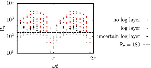
In summary, ${\mathsf{R}}_{}$ depends on the phase $\omega t$, the Reynolds number ${\mathsf{R}}_{\delta }$ and on the ratio $h/{\delta }_s$. From these dependences, it might be expected that the existence of the log-layer is only governed by ${\mathsf{R}}_{}$. However, this claim appears to be refuted by Fig. 12, in which the presence of the logarithmic layer is displayed as a function of ${\mathsf{R}}_{}$ and $\omega t$. At $\omega t=\pi /3$, no log-layer is detected for ${\mathsf{R}}_{}\mathsf{<}\mathsf{180}$, while a log-layer was already detected at this value of the Reynolds number in a plane-channel flow (Kim et al., 1987). In the region where the log-layer is present due to the local turbulence properties and not due to a history effect (i.e. from the start of the existence interval up to $\omega t<5\pi /12$), a threshold of about ${\mathsf{R}}_{}\mathsf{=}\mathsf{400}$ seems appropriate. However, for $\omega t=2\pi /3$ a log-layer is detected for ${\mathsf{R}}_{}\mathsf{<}\mathsf{180}$. These results suggest that once the log-layer enters the late deceleration phases, the threshold ${\mathsf{R}}_{}\mathsf{=}\mathsf{400}$ is not valid any more. In addition, at $\omega t=\pi /3$ and $\omega t=7\pi /12$, the log-layer is sometimes detected for lower values of ${\mathsf{R}}_{}$ than the values of ${\mathsf{R}}_{}$ for which the log-layer is not detected. These findings imply that it is not possible to reduce the number of parameters on which the presence of the log-layer depends, using ${\mathsf{R}}_{}$. As result, the log-layer in a turbulent oscillating flow cannot be analysed in a similar way as the log-layer in a steady turbulent flow, despite the similarities between the flows. To our current knowledge, the three parameters ${\mathsf{R}}_{\delta }$, $h/{\delta }_s$ and $\omega t$ are necessary for this analysis.

Figure 12. Link between the log-layer existence and the plane and phase averaged value of ${\mathsf{R}}_{}$. The threshold for which the log-layer has been identified in the plane channel flow of Kim et al. (1987), i.e. ${\mathsf{R}}_{}\mathsf{=}\mathsf{180}$, is also displayed

4. Discussion and conclusions

The present study confirms that a logarithmic region in the velocity profiles is present for oscillating flows, with a phase interval and a spatial extent that increases with the Reynolds number. A new identification method, the map of points of coordinates $(\ln (y_{vs}^{\mathtt{+}});⟨u(y_{vs}^{\mathtt{+}}⟩/U_0\left)\right)$, where $y_{vs}^{\mathtt{+}}$ is the thickness of the viscous viscosity dominated layer, demonstrates that the points of logarithmic velocity profiles collapse onto a single curve. This collapse makes the coordinates $(\ln (y_{vs}^{\mathtt{+}});⟨u(y_{vs}^{\mathtt{+}})⟩/U_0)$ a distinct signature of the logarithmic layer and can help to identify its presence.

This study also shows that the logarithmic layer is never present throughout the whole cycle at the values of the Reynolds number simulated in this investigation, in agreement with previous studies (Jensen et al., 1989; Salon et al., 2007). Nevertheless, the simulation results show that with increasing value of the Reynolds number, the log-layer appears earlier in the oscillation cycle and grows in spatial extent. Furthermore, the values of the von Kármán constant κ and the intercept B are found to be phase and Reynolds number dependent and to deviate by an order of 10% with respect to the classical values of $\kappa =0.41$ and B=5.5. This is particularly remarkable because previous studies (Akhavan et al., 1991; Pedocchi, Cantero, & García, 2011; Scandura et al., 2016; Tuzi & Blondeaux, 2008) reported a value of the von Kármán constant much closer to the classical value. However, these studies were carried out in pipe flows, and a study by Marusic et al. (2010) stated that the universality of the von Kármán constant depends on the type of flow (pressure driven flow, plane channel flow or pipe flow). Nevertheless, deviation of order 10% for κ and a decrease of B towards the end of the cycle was also reported by Salon et al. (2007). They attributed the decreasing value of B at the end of the deceleration phase, in the presence of an adverse pressure gradient, to a low-Reynolds number effect, but we believe that the presence of the log-layer at the end of the deceleration phase is just due to a history effect. Additionally, two other sources of discrepancies between different values of the log-layer constants might be considered. First, the mechanism of turbulence generation is not exclusively similar to that of steady wall-bounded flows, for low Reynolds number values: during the acceleration phase small disturbances are damped (Vittori & Verzicco, 1998) while turbulence at the end of the deceleration phase is generated by the collapse of the wall shear stress, due to the adverse pressure gradient, and not by the rigid wall itself (Jensen et al., 1989). This is only true for lower values of the Reynolds numbers. For high Reynolds number values, turbulence appears already during the acceleration phase (Jensen et al., 1989). Second, the method with which the von Kármán constant was determined (i.e. by taking the local minimum of the log-layer diagnostic function Ξ) might lead to a slight overestimation when compared to fitting a log-layer through the velocity profile (Jiménez & Moser, 2007; Pirozzoli et al., 2014). In fact, the present investigation demonstrates that when the fitting procedure was applied, the obtained values of κ and B could be much closer to the values reported in literature. However, the new values are then dependent on the size of the fitting interval. Therefore, the main result is that the values for κ and B strongly depend on three distinct parameters: ${\mathsf{R}}_{\delta }$, $h/{\delta }_s$ and the phase $\omega t$. To our current understanding, it is not possible to reduce the number of parameters on which the properties of the logarithmic layer depend, like a Reynolds number based on the friction velocity $u_{\tau }$.

Finally, the reduction of the ratio $h/{\delta }_s$ is found (i) to increase the phase interval for which intermittent turbulence is observed and (ii) to shift the existence interval of the log-layer to earlier phases. For these simulations characterized by intermittency, the presence of the logarithmic layer also depends on the oscillation cycle. Nevertheless, the values of the Reynolds numbers for the simulations presented here are relatively low for some applications. In tidal flows for example, Reynolds number values might be one order of magnitude higher (Kaptein et al., 2019), and we would expect the logarithmic layer to be present for a longer phase interval and the properties of the log-layer to be more constant.

Overall, we believe that the logarithmic assumption in wall models as formulated by Piomelli and Balaras (2002) is (i) a good approximation for oscillating flows at very high Reynolds number and (ii) an acceptable approximation at moderate Reynolds numbers. Nevertheless, if more accurate results need to be obtained, or for oscillating flows characterized by a strong reduction in turbulence activity or intermittent turbulence during (at least part of) the oscillation cycle, more sophisticated wall models are needed. These models should take into account the phase and Reynolds number dependence of (i) the existence of the log-layer and (ii) the values of the von Kármán constant and the intercept. Also, if a wall model is used the height above the bottom in wall units of the first computational point is crucial. Depending on the phase within the oscillation cycle it can either be in the viscous sub-layer or in the logarithmic region. Therefore, an accurate wall model would have to incorporate the entire law of the wall, i.e. $u^{\mathtt{+}}=y^{\mathtt{+}}$ in the viscous sub-layer, $u^{\mathtt{+}}=1/\kappa \ln \left(y^{\mathtt{+}}\right)+B$ in the log-layer, as well as an adequate parametrization of the buffer layer.

Notation

B	=	logarithmic layer intercept (–)
d	=	dynamic boundary layer thickness (m)
$E$	=	relative error between the velocity profile and the log-law (–)
h	=	water depth (m)
$L_x$	=	domain length in the x (steamwise) direction (m)
$L_z$	=	domain length in the z (spanwise) direction (m)
$n_x$	=	number of cells in the x (steamwise) direction (–)
$n_y$	=	number of cells in the y (vertical) direction (–)
$n_z$	=	number of cells in the z (spanwise) direction (–)
P	=	pressure (Pa)
${\overline{p}}^{\ast }$	=	non-dimensional, filtered pressure (–)
$P^{\ast }$	=	large-scale, non-dimensional pressure (–)
R	=	pipe radius (m)
${\mathsf{R}}_{\delta }$	=	Reynolds number based on the Stokes boundary layer thickness (–)
${\mathsf{R}}_{}$	=	Reynolds number based on the friction velocity (–)
t	=	time (s)
$t^{\ast }$	=	non-dimensional time (–)
$U_0$	=	amplitude of the free-stream velocity (m s${}^{-1}$ )
$u^{\mathtt{+}}$	=	non-dimensional, streamwise velocity (–)
${\overline{u}}_i^{\ast }$	=	non-dimensional, filtered velocity in the $x_i^{\ast }$ direction (–)
${\overline{u}}^{\ast }$	=	non-dimensional, filtered streamwise velocity (–)
$⟨u⟩$	=	ensemble averaged, streamwise velocity (m s${}^{-1}$)
$u_{\tau }$	=	friction velocity (m s${}^{-1}$)
$u_{\mathrm{\infty }}$	=	laminar infinite-depth solution (m)
${\overline{v}}^{\ast }$	=	non-dimensional, filtered vertical velocity (–)
${\overline{w}}^{\ast }$	=	non-dimensional, filtered spanwise velocity (–)
x	=	space variable in the streamwise direction (m)
$x^{\ast }$	=	non-dimensional space variable in the streamwise direction (–)
$x_i^{\ast }$	=	non-dimensional space variable in the i-direction (–)
y	=	space variable in the vertical direction (m)
$y^{\ast }$	=	non-dimensional space variable in the vertical direction (–)
$y^{\mathtt{+}}$	=	wall unit (–)
$y_{vs}^{\mathtt{+}}$	=	thickness of the viscous sub-layer in wall units (–)
$y_{\mathrm{m}\mathrm{i}\mathrm{n}}^{\mathtt{+}}$	=	smallest possible height in wall units at which the log-layer can exist (–)
$y_{\mathrm{m}\mathrm{a}\mathrm{x}}^{\mathtt{+}}$	=	largest possible height in wall units at which the log-layer can exist (–)
$y_c^{\mathtt{+}}$	=	centre of the log-layer (–)
$z^{\ast }$	=	non-dimensional space variable in the spanwise direction (–)
${\delta }_s$	=	Stokes boundary layer thickness (m)
${\delta }_{i1}$	=	Kronecker delta (m)
$\mathrm{\Delta }\omega t$	=	phase interval (–)
ϵ	=	maximum value of the error (–)
κ	=	von Kármán constant (–)
ν	=	kimematic viscosity (m${}^2$ s${}^{-1}$)
Ξ	=	log-layer diagnostic function (–)
ρ	=	density (kg m${}^{-3}$)
${\tau }_w$	=	wall shear stress (Pa)
${\tau }_{ij}^{\ast }$	=	non-dimensional subgrid scale stresses (–)
ω	=	angular frequency (s${}^{-1}$)
$\omega t$	=	phase of the free-stream velocity (rad)

Acknowledgements

The authors acknowledge Prof. B. Mutlu Sumer for giving access to the experimental data used to validate the simulations. The authors also acknowledge project PRACE, and particularly Dr John Donners, for improving the parallelization of the computer software, making the algorithm one order of magnitude faster. Finally, the authors thank the Netherlands Organization for Scientific Research (NWO) for providing computational time on the Surfsara supercomputing facilities.

Additional information

Funding

This research was funded by Stichting voor de Technische Wetenschappen (STW) now NWO/TTW (the Netherlands) through the project “Sustainable engineering of the Rhine region of freshwater influence” (# 12682).

Appendix. Log-layer diagnostic function in normal scaling

Figure 13. Reproduction of the profiles of Fig. 4. (a) logarithmic layer and (b) their associated log-layer diagnostic Ξ function in normal scaling for ${\mathsf{R}}_{\delta }\mathsf{=}\mathsf{990}$, $h/{\delta }_s=10$ and $\omega t=\pi /2$

References

- Afzal, N., & Yajnik, K. (1973). Analysis of turbulent pipe and channel flows at moderately large Reynolds number. Journal of Fluid Mechanics, 61(1), 23–31. doi: 10.1017/S0022112073000546
- Akhavan, R., Kamm, R. D., & Shapiro, A. H. (1991). An investigation of transition to turbulence in bounded oscillatory Stokes flows part 1. experiments. Journal of Fluid Mechanics, 225, 395–422. doi: 10.1017/S0022112091002100
- Andreas, E. L., Claffey, K. J., Jordan, R. E., Fairall, C. W., Guest, P. S., Persson, P. O. G., & Grachev, A. A. (2006). Evaluations of the von Kármán constant in the atmospheric surface layer. Journal of Fluid Mechanics, 559, 117–149. doi: 10.1017/S0022112006000164
- Armenio, V., & Piomelli, U. (2000). A lagrangian mixed subgrid-scale model in generalized coordinates. Flow, Turbulence and Combustion, 65(1), 51–81. doi: 10.1023/A:1009998919233
- Bernardini, M., Pirozzoli, S., & Orlandi, P. (2014). Velocity statistics in turbulent channel flow up to Reτ=4000. Journal of Fluid Mechanics, 742, 171–191. doi: 10.1017/jfm.2013.674
- Costamagna, P., Vittori, G., & Blondeaux, P. (2003). Coherent structures in oscillatory boundary layers. Journal of Fluid Mechanics, 474, 1–33. doi: 10.1017/S0022112002002665
- Frenzen, P., & Vogel, C. A. (1995). On the magnitude and apparent range of variation of the von Kármán constant in the atmospheric surface layer. Boundary-Layer Meteorology, 72(4), 371–392. doi: 10.1007/BF00709000
- Gross, T. F., & Nowell, A. R. M. (1983). Mean flow and turbulence scaling in a tidal boundary layer. Continental Shelf Research, 2(2-3), 109–126. doi: 10.1016/0278-4343(83)90011-0
- Hino, M., Kashiwayanagi, M., Nakayama, A., & Hara, T. (1983). Experiments on the turbulence statistics and the structure of a reciprocating oscillatory flow. Journal of Fluid Mechanics, 131, 363–400. doi: 10.1017/S0022112083001378
- Hoyas, S., & Jiménez, J. (2006). Scaling of the velocity fluctuations in turbulent channels up to Reτ=2003. Physics of Fluids, 18(1), 011702. doi: 10.1063/1.2162185
- Hsu, C. T., Lu, X., & Kwan, M. K. (2000). LES and RANS studies of oscillating flows over flat plate. Journal of Engineering Mechanics, 126(2), 186–193. doi: 10.1061/(ASCE)0733-9399(2000)126:2(186)
- Jensen, B. L., Sumer, B. M., & Fredsøe, J. (1989). Turbulent oscillatory boundary layers at high Reynolds numbers. Journal of Fluid Mechanics, 206, 265–297. doi: 10.1017/S0022112089002302
- Jiménez, J., & Moin, P. (1991). The minimal flow unit in near-wall turbulence. Journal of Fluid Mechanics, 225, 213–240. doi: 10.1017/S0022112091002033
- Jiménez, J., & Moser, R. D. (2007). What are we learning from simulating wall turbulence? Philosophical Transactions of the Royal Society of London A: Mathematical, Physical and Engineering Sciences, 365(1852), 715–732. doi: 10.1098/rsta.2006.1943
- Jonsson, I. G. (1980). A new approach to oscillatory rough turbulent boundary layers. Ocean Engineering, 7(1), 109–152. doi: 10.1016/0029-8018(80)90034-7
- Jonsson, I. G., & Carlsen, N. A. (1976). Experimental and theoretical investigations in an oscillatory turbulent boundary layer. Journal of Hydraulic Research, 14(1), 45–60. doi: 10.1080/00221687609499687
- Kaptein, S. J., Duran-Matute, M., Roman, F., Armenio, V., & Clercx, H. J. H. (2019). Effect of the water depth on oscillatory flows over a flat plate: from the intermittent towards the fully turbulent regime. Environmental Fluid Mechanics, 1–18. doi:10.1007/s10652-019-09671-3
- Kim, J., Moin, P., & Moser, R. (1987). Turbulence statistics in fully developed channel flow at low Reynolds number. Journal of Fluid Mechanics, 177, 133–166. doi: 10.1017/S0022112087000892
- Kundu, P. K., & Cohen, I. M. (2002). Fluid mechanics (2nd ed.). San Diego: Elsevier.
- Li, M., Sanford, L., & Chao, S. Y. (2005). Effects of time dependence in unstratified tidal boundary layers: results from large eddy simulations. Estuarine, Coastal and Shelf Science, 62(1-2), 193–204. doi: 10.1016/j.ecss.2004.08.017
- Marusic, I., McKeon, B. J., Monkewitz, P. A., Nagib, H. M., Smits, A. J., & Sreenivasan, K. R. (2010). Wall-bounded turbulent flows at high Reynolds numbers: recent advances and key issues. Physics of Fluids, 22(6), 065103. doi: 10.1063/1.3453711
- Marusic, I., Monty, J. P., Hultmark, M., & Smits, A. J. (2013). On the logarithmic region in wall turbulence. Journal of Fluid Mechanics, 716, R3. doi: 10.1017/jfm.2012.511
- Mckeon, B. J., Li, J., Jiang, W., Morrison, J. F., & Smits, A. J. (2004). Further observations on the mean velocity distribution in fully developed pipe flow. Journal of Fluid Mechanics, 501, 135–147. doi: 10.1017/S0022112003007304
- Mujal-Colilles, A., Christensen, K. T., Bateman, A., & Garcia, M. H. (2016). Coherent structures in oscillatory flows within the laminar-to-turbulent transition regime for smooth and rough walls. Journal of Hydraulic Research, 54(5), 502–515. doi: 10.1080/00221686.2016.1174960
- Nagib, H. M., & Chauhan, K. A. (2008). Variations of von Kármán coefficient in canonical flows. Physics of Fluids, 20(10), 101518. doi: 10.1063/1.3006423
- Nieuwstadt, F. T., Boersma, B. J., & Westerweel, J. (2016). Turbulence-introduction to theory and applications of turbulent flows. Switzerland: Springer.
- Pedocchi, F., Cantero, M. I., & García, M. H. (2011). Turbulent kinetic energy balance of an oscillatory boundary layer in the transition to the fully turbulent regime. Journal of Turbulence, 12, N32. doi: 10.1080/14685248.2011.587427
- Perry, A. E., & Li, J. D. (1990). Experimental support for the attached-eddy hypothesis in zero-pressure-gradient turbulent boundary layers. Journal of Fluid Mechanics, 218, 405–438. doi: 10.1017/S0022112090001057
- Piomelli, U., & Balaras, E. (2002). Wall-layer models for large eddy simulations. Annual Review of Fluid Mechanics, 34, 349–374. doi: 10.1146/annurev.fluid.34.082901.144919
- Pirozzoli, S., Bernardini, M., & Orlandi, P. (2014). Turbulence statistics in Couette flow at high Reynolds number. Journal of Fluid Mechanics, 758, 327–343. doi: 10.1017/jfm.2014.529
- Radhakrishnan, S., & Piomelli, U. (2008). Large-eddy simulation of oscillating boundary layers: Model comparison and validation. Journal of Geophysical Research: Oceans, 113, C02022. doi: 10.1029/2007JC004518
- Ramaprian, B. R., & Tu, S. W. (1983). Fully developed periodic turbulent pipe flow. part 2. the detailed structure of the flow. Journal of Fluid Mechanics, 137, 59–81. doi: 10.1017/S0022112083002293
- Salon, S., Armenio, V., & Crise, A. (2007). A numerical investigation of the Stokes boundary layer in the turbulent regime. Journal of Fluid Mechanics, 570, 253–296. doi: 10.1017/S0022112006003053
- Salon, S., Armenio, V., & Crise, A. (2009). A numerical (LES) investigation of a shallow-water, mid-latitude, tidally-driven boundary layer. Environmental Fluid Mechanics, 9, 525–547. doi: 10.1007/s10652-009-9122-y
- Scandura, P., Faraci, C., & Foti, E. (2016). A numerical investigation of acceleration-skewed oscillatory flows. Journal of Fluid Mechanics, 808, 576–613. doi: 10.1017/jfm.2016.641
- Scotti, A., & Piomelli, U. (2001). Numerical simulation of pulsating turbulent channel flow. Physics of Fluids, 13, 1367–1384. doi: 10.1063/1.1359766
- Skote, M. (2014). Scaling of the velocity profile in strongly drag reduced turbulent flows over an oscillating wall. International Journal of Heat and Fluid Flow, 50, 352–358. doi: 10.1016/j.ijheatfluidflow.2014.09.006
- Sleath, J. F. A. (1987). Turbulent oscillatory flow over rough beds. Journal of Fluid Mechanics, 182, 369–409. doi: 10.1017/S0022112087002374
- Tennekes, H., & Lumley, J. L. (1972). A first course in turbulence. Cambridge: MIT Press.
- Townsend, A. A. (1961). Equilibrium layers and wall turbulence. Journal of Fluid Mechanics, 11(1), 97–120. doi: 10.1017/S0022112061000883
- Tuzi, R., & Blondeaux, P. (2008). Intermittent turbulence in a pulsating pipe flow. Journal of Fluid Mechanics, 599, 51–79. doi: 10.1017/S0022112007009354
- Vittori, G., & Verzicco, R. (1998). Direct simulation of transition in an oscillatory boundary layer. Journal of Fluid Mechanics, 371, 207–232. doi: 10.1017/S002211209800216X
- Zang, Y., Street, R. L., & Koseff, J. R. (1994). A non-staggered grid, fractional step method for time-dependent incompressible Navier-Stokes equations in curvilinear coordinates. Journal of Computational physics, 114, 18–33. doi: 10.1006/jcph.1994.1146