Assessment of interfacial turbulence treatment models for free surface flows

Abstract

The modelling of complex free surface flows is challenging due to the mobility and deformability of the interface and air entrainment characteristics, which are highly affected by turbulence. With the framework of Reynolds averaged Navier–Stokes (RANS) models and the volume of fluid (VOF) method, turbulence quantities at the air–water interface tend to be over-estimated. In this study, interfacial turbulence treatment methods including the buoyancy modification model based on the simple gradient diffusion hypothesis (SGDH) and Egorov’s turbulence damping model are investigated. Furthermore, due to the unconditionally unstable characteristics of the standard k-ε turbulence model, the stabilized k-ε turbulence model is applied as a comparison. The turbulence attenuation performance using different interfacial turbulence treatment methods in the vicinity of the interface is compared and discussed for stratified flows and free overflow weirs for aerated and non-aerated nappe scenarios. The turbulence quantities and free surface profile under different flow conditions are validated against experimental data and an analytical model. The results show that for free surface waves, both the SGDH model and the turbulence damping model give strong improvements in turbulence production compared with the standard k-ε model. The SGDH model augments the turbulence kinetic energy (TKE) in the unstable stratification, leading to unphysical behaviour for the partially dispersed and separated flow.

Keywords:

• Air entrainment
• buoyancy modification
• CFD
• free overflow weirs
• free surface flows
• turbulence damping

1 Introduction

Turbulence plays an important role in the free surface flow simulation (e.g., free overflow) and its interactions with hydraulic structures (e.g., force calculation on a spillway, weir, breakwater, etc.) (Bricker et al., 2013; Patil et al., 2018). The major challenges encountered in describing free surface flows are associated with the mobility and deformability of the concurrent interface (Watanabe & Ebihara, 2001). The formation and growth of disturbances at the near-interface flow field with the significant discontinuity of fluids leads to a spatial and temporal change of interfacial configuration, which poses profound challenges for free surface flow modelling. In addition, different types of free surface flows show different flow patterns and interfacial configurations, which increases the complexity of numerical modelling. Large-scale turbulent free surface flows exist in most industrial and environmental systems. Generally, turbulence models, maturely employed for single phase flows, are directly applied in multi-phase flows and each phase is treated as in local equilibrium. However, the phase interaction and momentum exchange among phases cannot be revealed properly in this way, leading to unphysical predictions of the interface and turbulence. One of the well-known issues is the over-estimation of turbulence at large-scale interfaces within the framework of Reynolds averaged Navier–Stokes (RANS) models. The inability to adequately account for the effect of the interface using RANS turbulence models stems from the closure of the Reynolds stresses by the turbulent viscosity formulation, where a strong anisotropy cannot be represented by a scalar turbulence viscosity (Frederix et al., 2018). Furthermore, as one of the most widely applied interface capturing methods incorporated with RANS turbulence models, the volume of fluid (VOF) method defines the fluid properties near the interface as varying with volumetric fraction, and hence, the density gradient over several cells at the interface is solved continuously. However, the fluid density at the air–water interface should be discontinuous with an infinite density gradient, which generates a laminar regime, triggered by a redistribution of energy over the horizontal directions near the interface.

In order to suppress turbulence production near the air–water interface within the framework of RANS turbulence models that were originally designed for a single-phase flow, various strategies have been performed in conjunction with additional phenomenological terms to describe the phase interactions. Fan and Anglart (2020) developed a “varRhoTurbVOF” solver for variable density incompressible flows, in which an additional term is included in the RANS transport equations to deal with turbulence inconsistency issues at the interface. Devolder et al. (Devolder et al., 2017; Devolder, Troch, et al., 2018) proposed a buoyancy modified k-ω SST turbulence model based on the simple gradient diffusion hypothesis (SGDH) to prevent excessive wave damping at the air–water interface during wave propagation, wave breaking, and wave run-up around a monopole. Egorov et al. (2004) proposed a wall-like treatment at the two-phase flow interface by implementing a source term in the turbulence dissipation transport equation. Frederix et al. (2018) improved the Egorov turbulence damping model by retaining an interface-related length scale and extending it to the k-ε model, and proved the capability of the Egorov turbulence damping model for large-scale two-phase co-current channel interfacial turbulence prediction. Fan and Anglart (2019) developed an asymmetric treatment for the turbulence damping terms in Egorov’s model to consider the differences in turbulence production on each side of the interface. Kamath et al. (2019) included a specific turbulence dissipation term in the turbulence transport equation as a boundary condition at the free surface and examined the applicability to different flow conditions in open channels. Nakayama and Yokojima (2003) incorporated a damping factor associated with the free-surface fluctuation amplitude into two-equation models. Because of their accessibility to numerical implementation, these damping functions and buoyancy modification terms have been widely employed and validated in certain types of flows such as waves, co-current flows, and counter-current flows (Devolder, Stratigaki, et al., 2018; Larsen & Fuhrman, 2018; Li et al., 2018). Nevertheless, the characteristics and limitations of each interface treatment method have not yet been fully investigated under partially dispersed and separated flows such as free overflow weirs. Free overflow weir modelling is difficult because the complex jet dynamics and air entrainment characteristics are highly influenced by turbulence effects, and the limitations of the analytical and numerical models have been depicted. Disanayaka Mudiyanselage (2017) used a ballistic model to study the overflow nappe behaviour and validated it against experimental results, concluding the ballistic model experiences high deviations of nappe trajectory prediction caused by the low cavity pressure for the non-aerated conditions. Bricker et al. (2013) illustrated the inability to model non-aerated overflow using a 2-dimensional CFD model and speculated the capability of the standard k-ε turbulence model in high air entrainment and flow turbulence. Since turbulence plays an important role in the air entrainment mechanisms in the plunge pool, where the irregular jet surface promotes the formation of air bubbles removing air from the cavity, and affects the nappe evolution and deformation of the free surface, the performance of interfacial turbulence treatments for partially dispersed and separated flows are worthy of investigation. Furthermore, it is imperative to further compare and discuss the capabilities of each interfacial turbulence treatment method since the physical meaning of empirical coefficients is not clear. Understanding of multi-phase interface interaction as a function of interfacial turbulence treatment is essential for the fundamental design of hydraulic structures, as it determines the computational accuracy of fluid–structure interaction and flow characteristics.

In order to better predict the mechanisms of failure of hydraulic structures, the performance of the interfacial turbulence treatment methods should be evaluated and fully discussed. Therefore, in this study, the buoyancy modification model and Egorov’s turbulence damping model, as two typical and widely-used interface turbulence treatment models, are compared for interface performance assessment of free surface flows. The standard k-ε turbulence model, as the most commonly used RANS model, is applied to reveal the intrinsic limitations of implementing a single-phase flow turbulence model for two-phase flow simulations (Zou et al., 2022, 2023). Furthermore, due to the unconditionally unstable characteristics of the standard k-ε turbulence model for the nearly potential flow region beneath the free surface the stabilized k-ε turbulence model proposed by Larsen and Fuhrman (2018) is applied as a comparison. Since the limitations of the numerical models for partially dispersed and separated flows are well understood, but interfacial turbulence treatment methods for these types of flows have not been yet investigated, in this study the turbulence quantities of each model are examined in detail under stratified flows and partially dispersed and separated flows using examples of free surface waves and a free overflow weir, respectively. Since incompressible turbulence models for multiphase flows are not included in OpenFOAM (http://www.openfoam.com, n.d.) by default, in order to solve the issue of turbulence inconsistency, we implemented the buoyancy modification model into the varRhoTurbVOF solver within the framework of the open source CFD toolbox OpenFOAM version 2006.

This study is structured as follows. In Section 2, the theoretical background of turbulence models and interfacial turbulence treatment methods including the standard k-ε model, the stabilized k-ε model, the buoyancy modification model, and Egorov turbulence damping model are introduced. An analytical method for nappe trajectory prediction is explained. In Section 3, the set-up of numerical models for free surface waves and free overflow weirs are described. The capability of free surface flow modelling using the standard k-ε model, the buoyancy modification model, the stabilized k-ε model, and the turbulence damping model are compared and discussed in detail in Section 4.

2 Methodology

RANS turbulence models provide a good balance between computational efficiency and modelling accuracy, and hence, are widely used in engineering practice (Zou et al., 2021a). The k-ε turbulence model, as the most commonly used model in computational fluid dynamics (CFD), shows plausible performance in a wide range of engineering applications such as wave propagation, hydrodynamic force prediction, and broad-crested weir modelling (Haun et al., 2011; Zou et al., 2020a, 2020b, 2021b). In this section, the standard k-ε turbulence model, the stabilized k-ε model, and two typical interface turbulence treatment methods are introduced. In addition, in order to investigate the jet behaviour of free overflow weirs in Section 3.2 and validate the effectiveness of interfacial turbulence treatment methods, a ballistic model is examined for the nappe trajectory prediction.

2.1 The standard k-ε model

The standard k-ε model solves the turbulence quantities in two transport equations for multi-phase flow in OpenFOAM, given by: (1) $\{\begin{array}{l}{\displaystyle \frac{\mathrm{\partial }}{\mathrm{\partial }t}}\left(\alpha \rho k\right)+\mathrm{\nabla }\cdot \left(\alpha \rho uk\right)-{\mathrm{\nabla }}^2\left(\alpha \rho D_{k}k\right)=\alpha \rho G\\ -\left({\displaystyle \frac{2}{3}}\alpha \rho \mathrm{\nabla }\cdot uk\right)-\left(\alpha \rho {\displaystyle \frac{ϵ}{k}}k\right)+S_k\\ {\displaystyle \frac{\mathrm{\partial }}{\mathrm{\partial }t}}\left(\alpha \rho ϵ\right)+\mathrm{\nabla }\cdot \left(\alpha \rho uϵ\right)-{\mathrm{\nabla }}^2\left(\alpha \rho D_{ϵ}ϵ\right)={\mathsf{C}}_{\mathsf{1}}{\displaystyle \frac{ϵ}{k}}\alpha \rho G\\ -\left({\displaystyle \frac{2}{3}}{\mathsf{C}}_{\mathsf{1}}\alpha \rho \mathrm{\nabla }\cdot uϵ\right)-\left({\mathsf{C}}_{\mathsf{2}}\alpha \rho {\displaystyle \frac{ϵ}{k}}ϵ\right)+S_{ϵ}\end{array}$(1) where k is turbulent kinetic energy (TKE); ε is turbulent kinetic energy dissipation rate; u is the mean component of the velocity; ρ is density of the fluid phase; α is phase fraction of the given fluid phase; G is turbulent kinetic energy production rate due to the anisotropic part of the Reynolds-stress tensor; D_k and D_ε are effective diffusivity for k and ε, respectively. C₁ and C₂ are dimensionless user-adjustable parameters, here C₁ = 1.44 and C₂ = 1.92 (Mellor & Yamada, 1982); S_k and S_ε are source terms.

In eddy viscosity turbulence modelling, turbulent viscosity ν_t is defined as: (2) ${\nu }_t=C_{\mu }\frac{k^2}{ϵ}$(2) where C_μ is a model coefficient for the turbulent viscosity.

2.2 Turbulence inconsistency issue in OpenFOAM

Fan and Anglart (2020) pointed out that the category of incompressible turbulence models such as the standard k-ε model for VOF-based solvers in OpenFOAM has a turbulence inconsistency issue at the interface. In the VOF method, the fluid mixture density ρ_m and viscosity μ_m are determined by: (3) $\begin{array}{rl}{\rho }_m& =\alpha {\rho }_1+(1-\alpha ){\rho }_2\end{array}$(3) (4) $\begin{array}{rl}{\mu }_m& =\alpha {\mu }_1+(1-\alpha ){\mu }_2\end{array}$(4) where α is the volume fraction of the primary phase in a cell; subscripts 1 and 2 denote the primary and secondary phases, respectively.

OpenFOAM constructs turbulence models for incompressible flows by assuming that ρ is constant. Therefore, the TKE equation in Eq. (1) for incompressible flow in a given phase in OpenFOAM is written as: (5) $\frac{\mathrm{\partial }k}{\mathrm{\partial }t}+\mathrm{\nabla }\cdot \left(uk\right)-{\mathrm{\nabla }}^2\left(D_{k}k\right)=G-\left(\frac{2}{3}\mathrm{\nabla }\cdot uk\right)-ϵ+S_k$(5) However, based on the chain rule, TKE equation should be written as: (6) $\begin{array}{rl}& \frac{\mathrm{\partial }k}{\mathrm{\partial }t}+\mathrm{\nabla }\cdot \left(uk\right)-{\mathrm{\nabla }}^2\left(D_{k}k\right)\\ & =G-\left(\frac{2}{3}\mathrm{\nabla }\cdot uk\right)-ϵ+S_k+\frac{\mathrm{\nabla }{\rho }_m}{{\rho }_m}\left(D_k\mathrm{\nabla }k\right)\end{array}$(6) Note that an additional term $\mathrm{\nabla }{\rho }_m/{\rho }_m\left(D_k\mathrm{\nabla }k\right)$ arises and is not zero for the transition zone near the multi-phase flow interface. In order to solve the issue with turbulence modelling in isothermal VOF-based solvers, this extra diffusion term has been added in the TKE equation, named the “varRhoTurb” solver (Fan & Anglart, 2020).

2.3 The stabilized k-ε model

The standard k-ε model is unconditionally unstable in regions of nearly potential flow with finite strain, leading to exponential growth of the eddy viscosity and turbulent kinetic energy. Therefore, a new turbulence closure with stress-limiting features was proposed by Larsen and Fuhrman (2018), given by: (7) $\begin{array}{rl}{\nu }_t& =C_{\mu }\frac{k^2}{\widetilde{ϵ}},\widetilde{ϵ}=max\left(ϵ,{\lambda }_2\frac{{\mathsf{C}}_{\mathsf{2}}}{{\mathsf{C}}_{\mathsf{1}}}\frac{p_0}{p_{\mathrm{\Omega }}}ϵ\right)\end{array}$(7) (8) $\begin{array}{rl}{p}_0& =2S_{ij}{S}_{ij},S_{ij}=\frac{1}{2}\left(\frac{\mathrm{\partial }{u}_i}{\mathrm{\partial }{x}_j}+\frac{\mathrm{\partial }{u}_j}{\mathrm{\partial }{x}_i}\right)\end{array}$(8) (9) $\begin{array}{rl}{p}_{\mathrm{\Omega }}& =2{\Omega }_{ij}{\Omega }_{ij},{\Omega }_{ij}=\frac{1}{2}\left(\frac{\mathrm{\partial }{u}_i}{\mathrm{\partial }{x}_j}-\frac{\mathrm{\partial }{u}_j}{\mathrm{\partial }{x}_i}\right)\end{array}$(9) where λ₂ is an additional stress limiter coefficient; here λ₂= 0.1 is taken. S_ij, Ω_ij are the mean strain and rotation rate tensors, respectively. For a region of nearly potential flow, p_Ω << p₀.

2.4 Buoyancy modification model

The buoyancy force due to the large density difference at the free surface has a non-negligible effect on turbulence production, and the effect of buoyancy on turbulence should be accounted for. This is conventionally done by modifying the turbulence transport equations through an extra buoyancy source term. However, the turbulence production due to buoyancy is not included in the incompressible flow solvers of OpenFOAM.

The most common approach (Devolder et al., 2017) is to use the SGDH method as a source term G_b, given by: (10) $G_b=-\frac{{\mu }_t}{\mathsf{P}{\mathsf{r}}_{\mathsf{t}}}\frac{1}{{\rho }_m^2}\frac{\mathrm{\partial }{\rho }_m}{\mathrm{\partial }{x}_j}\left(\frac{\mathrm{\partial }{p}_m}{\mathrm{\partial }{x}_j}+{\rho }_{\mathrm{\infty }}{g}_j\right)$(10) where Pr_t is a turbulent Prandtl number, given by a constant value of 0.85.

Considering the expression can be reformulated in terms of temperature gradients based on the ideal gas law, the spatial derivative of ρ_m can be calculated by: (11) $\frac{\mathrm{\partial }{\rho }_m}{\mathrm{\partial }{x}_j}=-\frac{p_{\ast }}{R{T}_m^2}\frac{\mathrm{\partial }{T}_m}{\mathrm{\partial }{x}_j}=-\frac{{\rho }_m}{T_m}\frac{\mathrm{\partial }{T}_m}{\mathrm{\partial }{x}_j}$(11) where p_* is thermodynamic pressure and is constant in both time and space. R is the universal gas constant.

Therefore, the buoyancy source term G_b can be rewritten as: (12) $G_b=\frac{{\mu }_t}{\mathsf{P}{\mathsf{r}}_{\mathsf{t}}}\frac{1}{{\rho }_m{T}_m}\frac{\mathrm{\partial }{T}_m}{\mathrm{\partial }{x}_j}\left(\frac{\mathrm{\partial }{p}_m}{\mathrm{\partial }{x}_j}+{\rho }_{\mathrm{\infty }}{g}_j\right)$(12) If $\frac{\mathrm{\partial }{p}_m}{\mathrm{\partial }{x}_j}\ll {\rho }_{\mathrm{\infty }}{g}_j$ can be met for the reference density, the pressure derivative can be omitted and the Boussinesq approximation ρ_m ≈ ρ_∞ can be made, according to ideal gas law, Eq. (12) can be further simplified as: (13) $G_b=-g_j\frac{{\mu }_t}{\mathsf{P}{\mathsf{r}}_{\mathsf{t}}}\frac{1}{{\rho }_m}\frac{\mathrm{\partial }{\rho }_m}{\mathrm{\partial }{x}_j}$(13) According to Eq. (2), Eq. (13) can be rewritten as: (14) $G_b=-g_j\frac{C_{\mu }}{\mathsf{P}{\mathsf{r}}_{\mathsf{t}}}\frac{k^2}{ϵ}\frac{\mathrm{\partial }{\rho }_m}{\mathrm{\partial }{x}_j}$(14) The degree to which ε is affected by the buoyancy is determined by C_3ε. The calculation of C_3ε is given by (ANSYS, 2019): (15) $C_{3ϵ}=\text{tanh}\left|\frac{v}{u}\right|$(15) where v is the component of the flow velocity parallel to the gravitational vector; and u is the component of the flow velocity perpendicular to the gravitational vector.

The source term in the ε Eq. (1) is given by: (16) $G_{ϵ}=C_{1ϵ}\frac{ϵ}{k}{C}_{3ϵ}{G}_b$(16) However, the buoyancy production term using SGDH was found to underestimate the spreading rate of a thermal plume and to overestimate the spreading rate of stably-stratified flow (Yan & Holmstedt, 1999). In order to overcome the limitation, Daly and Harlow (1970) proposed buoyancy production in terms of the density gradient and velocity fluctuation correlation based on the generalized gradient diffusion hypothesis (GGDH). Van Maele and Merci (2006) compared the effect of buoyancy modification on turbulence kinetic energy production using both SGDH and GGDH for fire-driven flows and found that the realizable k-ε model with buoyancy modification using GGDH produces more accurate predictions. However, for free surface flow modelling, GGDH was shown to lead to failing simulations due to instability in the TKE equation (Devolder et al., 2017). Therefore, only the SGDH method is adopted in this research. In the context of the above turbulence treatment at the interface using the “varRhoTurb” solver, we modified the “varRhoTurb” solver by implementing the SGDH method in OpenFOAM version 2006. The modified transport equations considering the buoyancy production of turbulence for incompressible flow are written as: (17) $\{\begin{array}{l}{\displaystyle \frac{\mathrm{\partial }k}{\mathrm{\partial }t}}+\mathrm{\nabla }\cdot \left(uk\right)-{\mathrm{\nabla }}^2\left(D_{k}k\right)=G-({\displaystyle \frac{2}{3}}\mathrm{\nabla }\cdot uk)\\ -ϵ+{\displaystyle \frac{\mathrm{\nabla }{\rho }_m}{{\rho }_m}}\left(D_k\mathrm{\nabla }k\right)+G_b\\ {\displaystyle \frac{\mathrm{\partial }ϵ}{\mathrm{\partial }t}}+\mathrm{\nabla }\cdot \left(uϵ\right)-{\mathrm{\nabla }}^2\left(D_{ϵ}ϵ\right)={\mathsf{C}}_{\mathsf{1}}{\displaystyle \frac{ϵ}{k}}(G+C_{3ϵ}{G}_b)\\ -({\displaystyle \frac{2}{3}}{\mathsf{C}}_{\mathsf{1}}\mathrm{\nabla }\cdot uϵ)-\left({\mathsf{C}}_{\mathsf{2}}{\displaystyle \frac{ϵ}{k}}ϵ\right)\end{array}$(17)

2.5 Turbulence damping model

In regard to RANS models, the strong turbulence generation at the phase interface is unphysical. As the most widely applied turbulence damping model, a “wall-like” treatment near the interface to dampen turbulence proposed by Egorov et al. (2001) is assessed. Within the framework of OpenFOAM, a source term for turbulence dissipation equations is added to the turbulence transport equation based on Egorov’s model, given by: (18) $S_{\omega }=A_i\Delta n\text{β}{\rho }_i{\left(\frac{B6{\mu }_i}{\text{β}{\rho }_i\Delta n^2}\right)}^2$(18) where A_i is the interfacial area density for phase i; Δn is cell height normal to interface; β is the k-ω model closure coefficient of destruction term, which is equal to 0.075; B is the damping factor, here B = 10; μ_i is the viscosity of phase i; ρ_i is the density of phase i.

The interfacial area density for phase i, which is only activated at the interface, is given by: (19) $A_i=2{\alpha }_i|\mathrm{\nabla }{\alpha }_i|$(19) where α_i is the volume fraction of phase i; $|\mathrm{\nabla }{\alpha }_i|$ is the magnitude of the gradient of volume fraction.

Fan and Anglart (2019) pointed out that symmetric treatment for all phases is incorrect due to the always positive value of the turbulence damping term and proposed an asymmetric interface turbulence treatment method for air–water flows, given by: (20) $S_{\omega }=\delta A_w\Delta n\text{β}{\rho }_w{\left(\frac{B6{\mu }_w}{\text{β}{\rho }_w\Delta n^2}\right)}^2+A_a\Delta n\text{β}{\rho }_a{\left(\frac{B6{\mu }_a}{\text{β}{\rho }_a\Delta n^2}\right)}^2$(20) where δ is a factor considering the asymmetric damping effect caused by the interface and is written as: (21) $\delta =-\frac{{\rho }_w}{{\rho }_a}\frac{{\mu }_a^2}{{\mu }_w^2}$(21)

2.6 Ballistic model

Based on the theory of projectile motion (Chanson, 1996; Disanayaka Mudiyanselage, 2017), an analytical model for a fully-aerated nappe trajectory can be developed based on the following assumptions. (1) Gravity is the only external force acting on the nappe. (2) Before the nappe impinges on the pool of water, the horizontal velocity component of the flow remains constant. A sketch of the trajectory of the aerated nappe using the principle of a projectile is shown in Fig. 1.

Figure 1 Aerated nappe profile for steady overflows

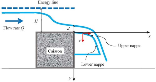
A theoretical parabolic nappe surface envelop of the lower nappe can be established, given by: (22) $\frac{y}{H}=\frac{gH}{2u^2}{\left(\frac{x}{H}\right)}^2$(22) The vertical component of thickness of the jet is constant due to the constant horizontal velocity. The upper nappe trajectory can be solved, given by: (23) $\frac{y}{H}=\frac{gH}{2u^2}{\left(\frac{x}{H}\right)}^2+\frac{d}{H}$(23) where u is the horizontal water particle velocity on the surface of the lower nappe, which can be estimated using the continuity equation downstream of the caisson top; H is the total head above the crest; d is the vertical thickness of the nappe; g is the gravitational acceleration. x and y are the nappe trajectory position in the horizontal and vertical directions, respectively. The coordinate system is established such that x is positive in the flow direction and y is positive in the downward direction.

3 Numerical model

Turbulence is a crucial physical phenomenon, particularly for wave breaking and wave–structure interaction. However, excessive wave height damping using single-phase incompressible turbulence models has been shown to lead to large discrepancies of wave run-up around monopiles and of the surface elevation of breaking waves (Devolder et al., 2017; Devolder, Troch, et al., 2018). In addition, overflow weirs, associated with complex jet dynamics and air entrainment characteristics, generate highly turbulent plunge pools with high rates of momentum transfer. Incompressible turbulence models designed for single-phase flows, such as the standard k-ε turbulent model and the realizable k-ε model, though widely used in skimming and nappe flow for spillway and weir modelling, are not completely satisfactory (Bilhan et al., 2018; Chinnarasri et al., 2014). In order to improve the turbulence reproduction performance and assess different interfacial turbulence treatment models for free surface flow prediction, free surface waves and overflow weirs are applied as case studies in this research.

3.1 Free surface waves

The surface wave is a typical two-phase separated flow where the deformability and structure of the two-phase interface are crucial factors. The influence of buoyancy on turbulence production is significant due to the large density ratio. Furthermore, a strong velocity gradient at the interface between two fluids results in strong turbulence generation in both phases in the standard turbulence model. Hence, turbulence damping is required in the interfacial area to model such flows correctly.

The reliability of the buoyancy modification approach near the air–water interface of waves has been proven (Devolder et al., 2017). However, the performance of different interface turbulence treatments in stratified flows has not yet been studied in sufficient depth. In this section, numerical wave models using the standard k-ε turbulent model, the turbulence damping model, and the buoyancy modification model (the SGDH model) are established. Furthermore, due to the unconditionally unstable characteristics of the standard turbulence model in the nearly potential flow region, the stabilized k-ε turbulence model is also applied. The buoyancy modification (SGDH model) was included in the stabilized k-ε turbulence model by Larsen and Fuhrman (2018). However, for the sake of evaluating the relative contributions of buoyancy modification vs. stabilization to the standard two-equation turbulence closure model in free surface wave prediction, stabilized k-ε turbulence models with and without buoyancy modification are applied as a comparison. Prediction of detailed turbulence quantities using each method is compared and discussed in Section 4.1.

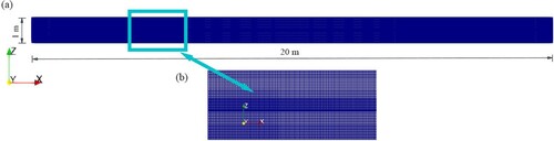
A two-dimensional numerical wave flume is generated using OpenFOAM. The computational domain is 20 m in length and 1 m in height with a water depth d of 0.5 m (Fig. 2). The wave height H and period T are 0.12 m and 2.0 s, respectively (hence wave steepness = 0.03; kd = 0.774; kH = 0.186, where k = 2π/L, L is the wavelength). Fifth order Stokes theory, regarded as sufficiently accurate, is adopted for the wave profile description. IHFOAM (Lara et al., 2013) is applied for wave simulations. At the inlet, the “activeAbsorption” function is activated and at the outlet, “shallowWaterAbsorption” is implemented. A no slip boundary at the bottom is applied, and standard wall functions are used at the bottom boundary for TKE, turbulence viscosity, and turbulence dissipation rate. The global cell size is 0.02 m in the vertical direction while it is refined near the air–water interface with a minimum cell size of 0.01 m. The total number of cells is 48,000. Results have been proven to be grid-size independent (Devolder et al., 2017). The total simulation time is 30 s.

Figure 2 (a) Computational domain of the numerical wave model; (b) mesh detail

3.2 Free overflow weirs

The overflow nappe involves complex overflow jet dynamics and air–water interactions, and often highly transient behaviour, which brings numerous challenges for numerical modelling. Research issues include pressure distributions behind the nappe and on the caisson, nappe trajectory predictions associated with cavity sub-pressure, and aeration and non-aeration effects. The interface modelling affects the mass and momentum exchange processes across the nappe and air, determining the accuracy of flow field properties and flow–structure interaction predictions. Scenarios can be categorized into a fully aerated nappe and a non-aerated nappe. The fully aerated nappe indicates both the upper and lower nappes are located at atmospheric pressure, while a non-aerated nappe occurs due to the formation of a sub-atmospheric pressure in the air cavity under the lower nappe.

In order to demonstrate and validate the behaviour of interfacial turbulence treatments in overflow nappe modelling, an experimental study of caisson overflow, acting as a broad-crested weir, is conducted in the hydraulics lab of the University of Michigan. The caisson is 0.3 m in height, 0.6 m in width and 0.3 m in length. The inflow rate Q is 50 m³ h⁻¹ (0.013889 m³ s⁻¹). Three pressure sensors are placed on the downstream surface of the caisson, located distances of 3.5, 8.5 and 26.5 cm above the caisson bottom, namely P1, P2 and P3, respectively. The top pressure sensor (P3) is used to measure the air suction within the cavity, and the other two pressure sensors (P1 and P2) are submerged downstream of the basin to measure water pressure variations. The measurement range for the water pressure sensors is 100 kPa, with a measurement accuracy of ± 100 Pa. The measurement range for the air pressure sensor is 746.52 Pa with a measurement accuracy of ± 15 Pa. In the experiments, the aerated condition is created by connecting a snorkel of PVC tubing through the caisson and up at the surface. The non-aerated condition is created by closing this tubing The experimental model set-up is shown in Fig. 3a.

Figure 3 Sketch of the free overflow weirs. (a) experimental set-up, P1 is the pressure sensor to measure water pressure near the bottom; P2 is the pressure sensor to measure water pressure near the water surface; P3 is the pressure sensor to measure air pressure within the cavity; (b) calculation domain of the numerical model

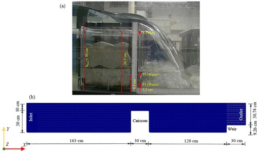
For the numerical models, a 2-dimensional numerical flume is generated for the fully-aerated nappe simulations. The computational domain is 3.43 m in length, 0.4 m in height, and 0.3 m in width. The caisson is placed at a distance of 1.63 m from the inlet. A weir with a height of 9.26 cm is placed downstream of the flume to control the outflow rate. The detailed dimensions of the numerical model are depicted in Fig. 3b. The grid resolution is 0.4 cm, which has been proven to be sufficient to capture the size and trajectory of the overflow nappe (Patil et al., 2018). In the Z (transverse) direction, a single cell is applied for 2-dimensional modelling. A coarse mesh with cell size in the X direction of 2 cm is applied near the outlet. The total number of cells is 68,315. The simulation is run for 30 s to assure that steady conditions have been reached. The left boundary is a specified velocity boundary based on the volumetric flow rate (a uniform velocity field normal to the inlet section adjusted to match the flow rate in the experiments). The right boundary is an outflow boundary where the flow quantities normal to the boundary have a zero gradient. The top boundary is the pressure inlet–outlet velocity boundary, which assigns a zero-gradient condition for flow out of the domain. In addition, a pressure inlet–outlet velocity boundary is applied at the top of the downstream wall of the caisson to allow simulation of a ventilated cavity under the jet. A no-slip hydraulically smooth wall condition is employed on the rest of the caisson surfaces and at the flume bottom. For the boundary at both sides, planes of symmetry (free-slip) are treated with zero viscous drag. For the discretization scheme settings, central discretization is selected for pressure gradient and diffusion terms; “Van Leer” is used for the divergence operators, and “Euler” is used for the time discretization. An adaptive time step is selected, and the maximum Courant number is set to 0.75. The PIMPLE algorithm, which combines the PISO and SIMPLE algorithms, is used for pressure-velocity coupling. A high-performance computing (HPC) cluster is applied to run parallel computation tasks.

For numerical modelling of the non-aerated nappe, 2-dimensional simulation has been proven inadequate as the simulated nappe clings to the caisson surface (Bricker et al., 2013). This is because there is no way for the air to get back into the space behind the nappe and contribute to the formation of instabilities in and under the nappe. Patil et al. (2018) resolved the overflow jet trajectory by employing a 3-dimensional numerical model with the interFoam solver and the standard k-ε model and revealed that the inability of 2-dimensional models to simulate non-aerated overflow is because the physics of aeration of the overflow jet cannot be adequately incorporated. Therefore, in this study, a 3-dimensional numerical model is established for the non-aerated nappe simulation. The experimental flume width in the Z (transverse) direction is 0.6 m. In the numerical model, the two side boundaries are set as a no-slip hydraulically smooth wall and a plane of symmetry, for a 0.3 cm wide simulation domain. The model runs for 30 s on a coarse mesh to assure a steady flow field is obtained, and then the results are interpolated onto a fine mesh from the prior time step by using the mapFields utility of OpenFOAM. The transient turbulence quantities are obtained by considering that steady conditions are reached after 10 s of simulation on the fine mesh. The total number of cells in the 3-dimensional model with the fine mesh is 5, 123, 625, which is considered to be sufficient according to the grid convergence study (Patil et al., 2018). Overflow jet modelling using the standard k-ε model, the turbulence damping model, and the SGDH model will be compared and discussed in Section 4.2.

4 Results

4.1 Free surface waves

Figure 4 illustrates the surface elevations in the wave flume using a laminar solution, the standard k-ε turbulence model, the stabilized k-ε turbulence model without buoyancy modification, the stabilized k-ε turbulence model with buoyancy modification (stabilized k-ε turbulence model + SGDH), the turbulence damping model, and the buoyancy modification model (the SGDH model), respectively. The wave signals propagate at the same initial time from the inlet, and the observation points are x = 5, 10, 15 and 17 m along the flume from the inlet. A clear surface elevation damping and wave phase shift using the standard k-ε model and the stabilized k-ε turbulence model without buoyancy modification can be observed. The relative errors on wave surface elevation predictions using different turbulence models at t = 5 and 17 s are listed in Table 1. The wave height damps about 3.3%, and the wave phase lags about 0.2 s at x = 17 m compared with the laminar solution. The turbulence damping model shows a better performance for wave height prediction. However, wave phase lag can be observed (e.g. x = 17 m, t = 24.5 s). The surface elevations and wave phases using the stabilized k-ε turbulence model with buoyancy modification and the SGDH model are generally consistent with the laminar results. This demonstrates that the buoyancy production term improves the surface wave simulation.

Figure 4 Time series of free surface elevation with respect to the bottom (z = 0 m) at downstream distances (a) x = 5 m; (b) x = 10 m; (c) x = 15 m; (d) x = 17 m

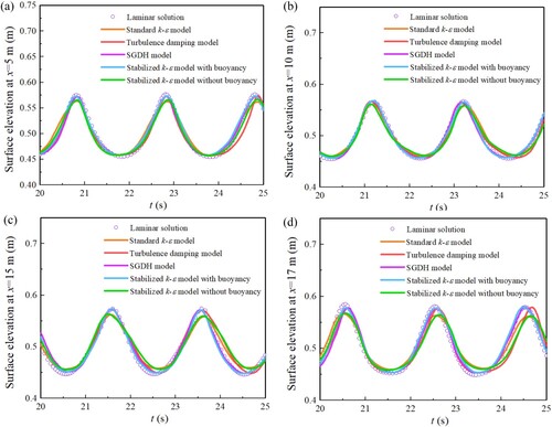
Table 1 Relative errors on wave surface elevation predictions using different turbulence models

	t = 5s		t = 17s
Model	Peak surface elevation (m)	Relative error (=|laminar value – model value|/laminar value × 100%)	Peak surface elevation (m)	Relative error (=|laminar value – model value|/laminar value × 100%)
Laminar	0.577		0.582
Standard k-ε model	0.563	2.4	0.563	3.3
Stabilized k-ε model	0.566	1.9	0.565	2.9
Stabilized k-ε + SGDH	0.573	0.7	0.577	0.9
Turbulence damping model	0.573	0.7	0.575	1.2
SGDH model	0.573	0.7	0.577	0.9

The phase volume fraction, TKE, turbulence dissipation rate, and turbulent viscosity at t = 25 s in the flume are depicted in Fig. 5 for the standard k-ε turbulence model, the stabilized k-ε turbulence model without buoyancy modification, the stabilized k-ε turbulence model with buoyancy modification (stabilized k-ε turbulence model + SGDH), the turbulence damping model, and the SGDH model, respectively.

Figure 5 Turbulent quantities at t = 25 s using different turbulence treatment methods (instantaneous results). (a) Phase volume fraction, alpha.water = 1 is water phase, alpha.water = 0 is air phase, 0 < alpha.water < 1 is mixed air and water; (b) TKE; (c) turbulence dissipation rate; (d) turbulent viscosity

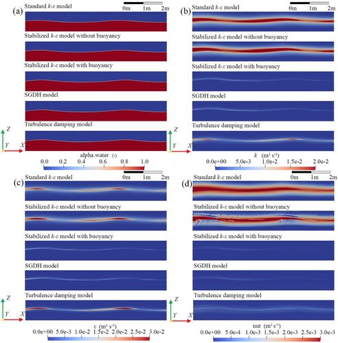
The wave elevation and phase are generally consistent for different models (Fig. 5a). From Fig. 5b, both the standard model and stabilized k-ε turbulence model without buoyancy show large TKE at the air–water interface. The turbulence damping model shows less TKE at the interface, while the SGDH model and the stabilized k-ε turbulence model with buoyancy modification have the lowest TKE at this location. The reduction of TKE using the SGDH model can be attributed directly to the interfacial turbulence suppression with the buoyancy modification term in Eq. (17). For the turbulence damping model, based on the TKE transport equation, the increased turbulence dissipation near the interface can lead to a TKE reduction. However, it is noted that TKE reduction using the turbulence damping model is not as effective as the SGDH method. Likewise, from Fig. 5c, large turbulence dissipation can be observed in the standard and stabilized k-ε turbulence models without buoyancy modification. Furthermore, a clear enhancement of turbulence dissipation rate can be observed for the turbulence damping model due to the added turbulence dissipation source term in Eq. (20). However, the difference in turbulence dissipation rate between the SGDH model and the stabilized k-ε turbulence model with buoyancy modification is not obvious. From Fig. 5d, the SGDH model, the stabilized k-ε turbulence model with buoyancy modification, and the turbulence damping model produce obvious improvement in turbulence production at the air–water interface compared with the standard model and stabilized k-ε model without buoyancy modification. The SGDH and turbulence damping methods deal with the suppression of turbulence quantities near the large-scale interface in different ways. According to the eddy viscosity model in Eq. (2), for the turbulence damping model, the increased turbulence dissipation and decreased TKE at the interface leads to a reduction of turbulence viscosity. While in the SGDH model, the turbulence viscosity at the interface decreases due to the reduction of TKE. However, this demonstrates that the SGDH model more effectively reduces the turbulence viscosity at the interface than the turbulence damping model does. The over-predicted turbulent viscosity at the air–water interface by using the standard model and stabilized k-ε model without buoyancy modification is the main reason for the wave amplitude damping and phase shift in Fig. 4.

The turbulent viscosity at one wavelength for the SGDH model and the “stabilized k-ε turbulence model with buoyancy” (stabilized k-ε turbulence model + SGDH) is further examined in Fig. 6, to investigate the effects of stabilized modification to the standard model in turbulence prediction. It depicts that the excessive turbulence production is only constrained at the free surface (the blue line) by the SGHD model, while the turbulent viscosity is limited with the magnitude of kinematic fluid viscosity in the nearly potential flow region (beneath the free surface and above the bottom boundary layer) by the “stabilized k-ε turbulence model with buoyancy”. It proves that the instability of the standard two-equation turbulence model leads to a growth of the eddy viscosity, and the stabilizing modification can effectively eliminate the unphysical growth of turbulence.

Figure 6 Turbulent kinematic viscosity at t = 25 s using the SGDH model and the stabilized k-ε model with buoyancy

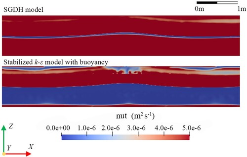
It should be noted that the buoyancy modification primarily deals with surface-related problems, which may manifest more rapidly but have a localized impact. On the other hand, stabilizing the eddy viscosity aims to prevent the exponential growth of turbulence below the surface (Larsen & Fuhrman, 2018). It is essential to consider the complementary nature of the two features in nearly potential flow scenarios such as free surface waves.

4.2 Free overflow weirs

Except for a region of nearly potential flow, the stabilized k-ε model is identical to the standard k-ε model (Eq. 7). Therefore, for the shear flow regions of free overflow weirs, only the standard k-ε model, the turbulence dissipation model, and the SGDH model are compared and discussed.

Fully-aerated nappe

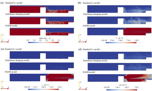
The phase volume fraction, TKE, turbulence dissipation rate, and turbulent viscosity at steady state are depicted in Fig. 7 for the standard k-ε model, the turbulence dissipation model and the SGDH model, respectively. It shows the turbulence quantities solved by the standard k-ε model and the turbulence damping model are small and the difference between them is minor. However, the TKE, turbulence dissipation rate, and turbulent viscosity using the SGDH model are highly over-predicted downstream of the overflow weir (Fig. 7b, c and d). According to Eq. (14), buoyancy tends to suppress the turbulence only for stable stratification (G_b < 0 at the interface). However, the lower nappe of the overflow jet is above an air cavity, and thus unstable stratification exists (G_b > 0). Furthermore, the density gradient at the air–water mixing region is discontinuous due to the entrainment of discrete droplets of water phase into the air, and the entrainment of air bubbles into the water column; hence, TKE is augmented in the region of unstable stratification (G_b > 0). Unlike buoyancy-driven flows due to temperature variations such as fire-generated flows, where the TKE increases when the temperature gradient of the buoyant plume is opposite to the direction of gravity and vice versa, this treatment causes unphysical and unrealistic flow behaviour for unstable partially dispersed and separated flows stemming from the dispersed individual particles moving in time and space. With the air entrainment by the entering jet, the velocity of individual drops of water slows down due to air drag, and the inner jet core should disintegrate due to impact with the flume floor (Castillo et al., 2015). However, the water drops coalesce into a bunch after the entering jet hits the flume floor, and the diffusion process cannot be observed by the SGDH model.

Figure 7 Turbulence quantities of fully-aerated nappe flow at t = 30 s using different turbulence treatment methods. (a) Phase volume fraction, alpha.water = 1 is water phase, alpha.water = 0 is air phase, 0 < alpha.water < 1 is mixing air and water; (b) TKE; (c) turbulence dissipation rate; (d) turbulence viscosity

Turbulence affects the jet break-up and air entrainment characteristics, and further affects the pressure prediction. Figure 8a, b and c show a comparison of the pressure time series between the numerical results and experimental data at the three pressure sensors of Fig. 3. All the numerical models reveal the presence of pressure fluctuations due to the intense air entrainment and entrapment process in the jet impingement area. Since the fluctuating pressure is determined by the jet behaviour and the flow recirculation under the nappe in the water, owing to the high turbulent viscosity predicted by the SGDH model, the fluctuating pressure is smaller with a higher fluctuation frequency than the other models. The large scatter of the experimental data can be observed in Fig. 8a and b, which can be attributed to the measurement precision of the water pressure sensors. Since a pressure gradient in the snorkel tube is necessary to suck air into the cavity in the experiments, it is difficult to establish a fully-aerated scenario, and hence, it turns out to be a partially aerated nappe with a slightly sub-atmospheric pressure in the cavity. This leads to a lower pressure in the experiments than the numerical results, where atmospheric pressure was specified directly on the portion of the downstream surface of the caisson within the air cavity.

Figure 8 Comparison of pressure on the downstream face of the caisson and nappe trajectory using experimental data, ballistic model, the standard k-ε model, the turbulence dissipation model and the SGDH model for a fully-aerated nappe (a) bottom water pressure; (b) top water pressure; (c) air pressure; (d) nappe trajectory (the numerical data are instantaneous when the nappe trajectory is steady)

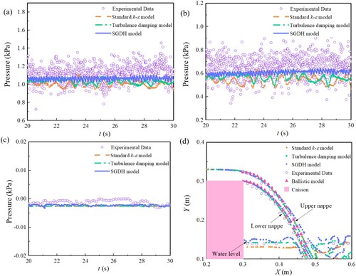
In Fig. 8d, the air–water interface and water level under the jet are extracted from the numerical model and the results are validated against the ballistic model and experimental data. The trajectory of the jet using all the selected models shows good agreement with the experimental data and analytical results. However, slight deviations of the lower nappe trajectories can be observed between the numerical results and the experimental data, revealing that the horizontal flow velocity on the surface of the lower nappe in the experiments is smaller than in the numerical models, due to the presence of caisson roughness in the experiments. In addition, due to the partially aerated conditions of the experiments, the sub-atmospheric pressure inside the cavity pulls the lower nappe trajectory slightly towards the caisson. However, the upper nappe trajectory can be perfectly predicted since the mean flow motion there represents the bulk flow. Both the standard k-ε model and the turbulence damping model show good accuracy in predicting the overflow jet’s upper nappe trajectory. However, the SGDH model deviates from the other models and has a larger falling jet thickness near the impingement area. The water levels below the jet using the turbulence damping model are in very good agreement with the experimental data. However, water levels under the jet are slightly under-predicted using the standard k-ε model.

Non-aerated nappe

The phase volume fraction, TKE, turbulence dissipation rate, and turbulent viscosity at the steady state (t = 10 s on the fine mesh) are depicted in Fig. 9 for the standard k-ε model and the turbulence damping model. Due to the unphysical turbulence quantities predicted by the SGDH model, however, the SGDH simulation failed at 2.4 s on the fine mesh with a large continuity error. Therefore, the phase volume fraction, TKE, turbulence dissipation rate, and turbulent viscosity using the SGDH model at the simulation time of 2.4 s are shown in Fig. 9 for comparison. Similar to the fully-aerated nappe scenario, the turbulence quantities predicted by the SGDH model are much larger than the standard k-ε model and the turbulence damping model. The TKE and turbulent viscosity using the turbulence damping model are effectively attenuated compared with the standard k-ε model. Furthermore, once the flow accelerates on top of the caisson, large turbulence dissipation develops next to the upstream end of the weir crest in the standard k-ε model, whereas large turbulence dissipation occurs until the jet impinges the tailwater and evolves downstream in the turbulence damping model. It can also be observed from Fig. 9b, c and d that in the turbulence damping model, larger TKE and turbulent viscosity occur at the centreline of the nappe than at the side wall. This is due to the presence of the wall restricting the development of large vortices. However, it is not obvious in the standard k-ε model.

Figure 9 Turbulence quantities of the non-aerated nappe at t = 10 s using different turbulence treatment methods. (a) Phase volume fraction, alpha.water = 1 is water phase, alpha.water = 0 is air phase, 0 < alpha.water < 1 is mixing air and water; (b) TKE; (c) turbulence dissipation rate; (d) turbulence viscosity

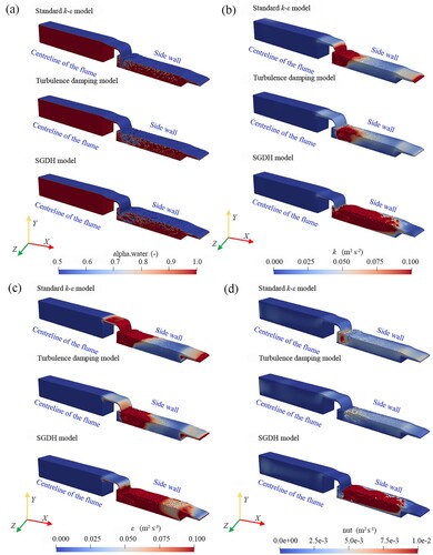
Figure 10a, b and c shows the comparison between the numerical results and experimental data of the time series of the three pressure sensors for the non-aerated cases. Since the unrealistic turbulence quantities predicted by the SGDH model lead to failing simulations, only results using the standard k-ε model and the turbulence dissipation model are presented. For the mean pressures in the water column under the jet, both of the numerical models show good agreement with the experiment. For the sub-atmospheric pressure prediction in the air cavity, the turbulence damping model shows a satisfactory agreement with the experimental results, while the standard k-ε model over-estimates the negative pressure within the cavity. In addition, the fluctuation of pressure based on the turbulence damping model is smaller than the standard k-ε model.

Figure 10 Comparison of pressure on the rear of the caisson surface and nappe trajectory using experimental data, ballistic model, the standard k-ε model, the turbulence dissipation model and the SGDH model for a non-aerated nappe (a) bottom water pressure sensor; (b) top water pressure sensor; (c) air pressure sensor; (d) nappe trajectory (the numerical data are instantaneous when the nappe trajectory is steady)

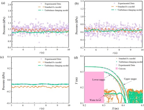
The nappe trajectory is obtained from a longitudinal slice of the 3-dimensional numerical model along the centreline of the flume. Figure 10d shows the numerical results of the lower and upper nappe trajectories and water level under the jet compared with the experimental data. A larger curvature of the jet trajectory and higher water level below the jet using the standard k-ε model can be observed compared with the experiment, due to the over-predicted negative sub-atmospheric pressure within the cavity (Fig. 10c), which pulls the jet towards the caisson and raises the water level below the jet. The turbulence damping model predicts pressure and water level better than the standard k-ε model and the nappe trajectory deviation is reduced. A more severe air entrainment process in the water (where air bubbles can be detected) is observed under and downstream of the jet with the standard k-ε model than with the turbulence damping model, which is consistent with the observations of larger fluctuation of pressure in Fig. 10a, b and c.

4.3 Discussion

It should be noted that within the framework of the RANS modelling technique, only the mean flow features can be captured. Despite the improvements in turbulence quantity predictions by the turbulence damping model, minor deviations of pressure, nappe trajectory and water level can still be observed. This is ascribed to the fact that those parameters are highly related to bubble formation, surface tension effects, and small-scale eddy flows in the air entrainment mechanisms, which cannot be properly resolved by the RANS modelling technique. This indicates the limitations of RANS modelling when dealing with complex, unsteady air entrainment characteristics and turbulence effects. In addition, the applied grid resolution of the simulations is still insufficient to resolve small-scale air bubbles and turbulent features. Therefore, the effects of viscous forces and surface tension on bubble calculations should be properly considered for flows with energetic air entrainment.

5 Conclusion

Turbulence over-estimation at the interface of free surface flows within the RANS modelling technique is a well-known issue. Therefore, turbulence should be attenuated at the interface. In this paper, typical interfacial turbulence treatment methods including the Egorov turbulence damping model and the buoyancy modification model are evaluated for free surface flows. Furthermore, the performance of the stabilized k-ε model for free surface wave prediction is compared and discussed. The open source CFD toolbox OpenFOAM is applied to simulate free surface waves and free overflow weirs for aerated and non-aerated nappes. The free surface profiles (e.g. wave amplitude and phase, nappe trajectory) and turbulence quantities (e.g. TKE, turbulence dissipation and turbulent viscosity) using the standard k-ε model, the turbulence dissipation model, and the SGDH model are analysed and compared to the experimental data and analytical results. The main conclusions are summarized as follows:

1. The over-predicted turbulent viscosity using the standard k-ε model induces a large momentum diffusion in the vicinity of the interface and in both phases, leading to unrealistic predictions such as a damped wave amplitude and phase shift.

2. For stable stratification, both the SGDH model and turbulence damping model produce obvious improvements in turbulence production at the air–water interface. The buoyancy modification results in better wave elevation and phase prediction than the turbulence damping model does.

3. The stabilizing modification to the standard two-equation turbulence closure model can successfully eliminate the unphysical growth of turbulence in the nearly potential flow region. Considering the effects of both buoyancy and stabilizing modifications is crucial in nearly potential flow scenarios.

4. The aerated nappe trajectory and pressure in the cavity and water column under the jet can be adequately predicted by both the standard k-ε model and the turbulence damping model using 2-dimensional numerical modelling. For unstable stratification such as partially dispersed and separated flows, the SGDH model largely over-estimates turbulence quantities, causing unphysical and unrealistic results.

5. For non-aerated weir flow, predictions of the nappe trajectory and water column elevation under the jet can be improved by using the turbulence damping model. However, small-scale eddies and air bubbles were not sufficiently resolved by the applied grid resolution and 2-dimensional nature of a portion of the simulations. Therefore, deviations of the nappe trajectory and pressure with the experiments are observed.

This study discussed the typical interfacial treatment methods based on the framework of RANS modelling and the VOF method. A more precise and better resolved turbulence prediction method for complex air entrainment mechanisms should be investigated in follow-on research. Additionally, to reproduce and validate the numerical results more effectively, specific turbulence characteristics (e.g. TKE, turbulence dissipation) should be rigorously measured in future experiments.

Notation

d	=	the vertical thickness of the nappe (m)
Dk	=	effective diffusivity for k (m2 s−1)
Dε	=	effective diffusivity for ε (m2 s−1)
g	=	the gravitational acceleration (m s−2)
G	=	turbulent kinetic energy production rate due to the anisotropic part of the Reynolds-stress tensor (m2 s−3)
H	=	the total head above the crest; wave height (m)
k	=	turbulent kinetic energy per unit mass (m2 s−2)
L	=	the wavelength (m)
Q	=	inflow rate (m3 s−1)
T	=	wave period (s)
u	=	fluid velocity; the horizontal water particle velocity on the surface of the lower nappe (m s−1)
x	=	the nappe trajectory position in the horizontal direction (m)
y	=	the nappe trajectory position in the vertical direction (m)
α	=	phase fraction of the given fluid phase (–)
ε	=	turbulent kinetic energy dissipation rate (m2 s−3)
νt	=	turbulent viscosity (m2 s−1)
ρ	=	density of the fluid phase (kg m−3)

Disclosure statement

No potential conflict of interest was reported by the author(s).

References

- ANSYS, F. (2019). ANSYS fluent theory guide 19.1. ANSYS.
- Bilhan, O., Aydin, M. C., Emiroglu, M. E., & Miller, C. J. (2018). Experimental and CFD Analysis of Circular Labyrinth Weirs. Journal of Irrigation and Drainage Engineering, 144(6), https://doi.org/10.1061/(asce)ir.1943-4774.0001301
- Bricker, J. D., Takagi, H., & Mitsui, J. (2013). Turbulence Model Effects on VOF Analysis of Breakwater Overtopping during the 2011 Great East Japan Tsunami. The 35th World Congress of the International Association for Hydro-Environment Engineering and Research (IAHR), September 8–13, 2013 Chengdu, Southwestern China.
- Castillo, L. G., Carrillo, J. M., & Blázquez, A. (2015). Plunge pool dynamic pressures: A temporal analysis in the nappe flow case. Journal of Hydraulic Research, 53(1), https://doi.org/10.1080/00221686.2014.968226
- Chanson, H. (1996). Air bubble entrainment in free-surface turbulent shear flows. Elsevier. https://doi.org/10.1016/b978-0-12-168110-4.x5000-0
- Chinnarasri, C., Kositgittiwong, D., & Julien, P. Y. (2014). Model of flow over spillways by computational fluid dynamics. Proceedings of the Institution of Civil Engineers: Water Management, 167(3), https://doi.org/10.1680/wama.12.00034
- Daly, B. J., & Harlow, F. H. (1970). Transport equations in turbulence. Physics of Fluids, 13(11), https://doi.org/10.1063/1.1692845
- Devolder, B., Rauwoens, P., & Troch, P. (2017). Application of a buoyancy-modified k-ω SST turbulence model to simulate wave run-up around a monopile subjected to regular waves using OpenFOAM®. Coastal Engineering, 125, https://doi.org/10.1016/j.coastaleng.2017.04.004
- Devolder, B., Stratigaki, V., Troch, P., & Rauwoens, P. (2018). CFD simulations of floating point absorber wave energy converter arrays subjected to regular waves. Energies, 11(3), https://doi.org/10.3390/en11030641
- Devolder, B., Troch, P., & Rauwoens, P. (2018). Performance of a buoyancy-modified k-ω and k-ω SST turbulence model for simulating wave breaking under regular waves using OpenFOAM®. Coastal Engineering, 138, https://doi.org/10.1016/j.coastaleng.2018.04.011
- Disanayaka Mudiyanselage, S. (2017). Effect of Nappe Non-aeration on Caisson Sliding Force during Tsunami Breakwater Overtopping.
- Egorov, Y., Boucker, M., Martin, A., Pigny, S., Scheuerer, M., & Willemsen, S. (2001). Validation of CFD codes with PTS-relevant test cases. 5th Euratom Framework Programme 1998–2002. European Commission, Key action: Nuclear Fission.
- Fan, W., & Anglart, H. (2019). Progress in phenomenological modeling of turbulence damping around a two-phase interface. Fluids, 4(3), https://doi.org/10.3390/fluids4030136
- Fan, W., & Anglart, H. (2020). varRhoTurbVOF: A new set of volume of fluid solvers for turbulent isothermal multiphase flows in OpenFOAM. Computer Physics Communications, 247, https://doi.org/10.1016/j.cpc.2019.106876
- Frederix, E. M. A., Mathur, A., Dovizio, D., Geurts, B. J., & Komen, E. M. J. (2018). Reynolds-averaged modeling of turbulence damping near a large-scale interface in two-phase flow. Nuclear Engineering and Design, 333, https://doi.org/10.1016/j.nucengdes.2018.04.010
- Haun, S., Olsen, N. R. B., & Feurich, R. (2011). Numerical modeling of flow over trapezoidal broad-crested weir. Engineering Applications of Computational Fluid Mechanics, 5(3), https://doi.org/10.1080/19942060.2011.11015381
- http://www.openfoam.com. (n.d.). OpenFOAM version 2006.
- Kamath, A., Fleit, G., & Bihs, H. (2019). Investigation of free surface turbulence damping in RANS simulations for complex free surface flows. Water (Switzerland), 11(3), https://doi.org/10.3390/w11030456
- Lara, J. L., Higuera, P., Guanche, R., & Losada, I. J. (2013). Wave interaction with piled structures: Application with ih-foam. Proceedings of the International Conference on Offshore Mechanics and Arctic Engineering - OMAE, 7. https://doi.org/10.1115/OMAE2013-11479
- Larsen, B. E., & Fuhrman, D. R. (2018). On the over-production of turbulence beneath surface waves in Reynolds-averaged Navier-Stokes models. Journal of Fluid Mechanics, 853, https://doi.org/10.1017/jfm.2018.577
- Li, M., Xie, L., Zong, X., Zhang, S., Zhou, L., & Li, J. (2018). The cruise observation of turbulent mixing in the upwelling region east of Hainan Island in the summer of 2012. Acta Oceanologica Sinica, 37(9), 1–12. https://doi.org/10.1007/s13131-018-1260-y
- Mellor, G. L., & Yamada, T. (1982). Development of a turbulence closure model for geophysical fluid problems. Reviews of Geophysics, 20(4), https://doi.org/10.1029/RG020i004p00851
- Nakayama, A., & Yokojima, S. (2003). Modeling free-surface fluctuation effects for calculation of turbulent open-channel flows. Environmental Fluid Mechanics, 3(1), https://doi.org/10.1023/A:1021136912983
- Patil, A., Mudiyanselage, S. D., Bricker, J. D., Uijttewaal, W., & Keetels, G. (2018). Effect OF OVERFLOW NAPPE NON-AERATION ON TSUNAMI BREAKWATER FAILURE. Coastal Engineering Proceedings, 36, https://doi.org/10.9753/icce.v36.papers.18
- Van Maele, K., & Merci, B. (2006). Application of two buoyancy-modified k-ε turbulence models to different types of buoyant plumes. Fire Safety Journal, 41(2), https://doi.org/10.1016/j.firesaf.2005.11.003
- Watanabe, T., & Ebihara, K. (2001, April). Parallel computation of rising bubbles using the lattice Boltzmann method on workstation cluster. In Parallel Computational Fluid Dynamics: Trends and Applications: Proceedings of the Parallel CFD 2000 Conference (p. 399). North-Holland.
- Yan, Z., & Holmstedt, G. (1999). A two-equation turbulence model and its application to a buoyant diffusion flame. International Journal of Heat and Mass Transfer, 42(7), https://doi.org/10.1016/S0017-9310(98)00206-3
- Zou, P., Bricker, J. D., & Uijttewaal, W. (2021a). Submerged floating tunnel cross-section analysis using a transition turbulence model. Journal of Hydraulic Research, https://doi.org/10.1080/00221686.2021.1944921
- Zou, P., Bricker, J., & Uijttewaal, W. (2020a). Optimization of submerged floating tunnel cross section based on parametric Bézier curves and hybrid backpropagation - genetic algorithm. Marine Structures, 74, https://doi.org/10.1016/j.marstruc.2020.102807
- Zou, P. X., Bricker, J. D., Chen, L. Z., Uijttewaal, W. S. J., & Simao Ferreira, C. (2022). Response of a submerged floating tunnel subject to flow-induced vibration. Engineering Structures, 253, https://doi.org/10.1016/j.engstruct.2021.113809
- Zou, P. X., Bricker, J. D., & Uijttewaal, W. S. J. (2020b). Impacts of extreme events on hydrodynamic characteristics of a submerged floating tunnel. Ocean Engineering, 218, https://doi.org/10.1016/j.oceaneng.2020.108221
- Zou, P. X., Bricker, J. D., & Uijttewaal, W. S. J. (2021b). The impacts of internal solitary waves on a submerged floating tunnel. Ocean Engineering, 238, 109762. doi:10.1016/j.oceaneng.2021.109762
- Zou, P. X., Ruiter, N., Bricker, J. D., & Uijttewaal, W. S. J. (2023). Effects of roughness on hydrodynamic characteristics of a submerged floating tunnel subject to steady currents. Marine Structures, 89, 103405. https://doi.org/10.1016/j.marstruc.2023.103405