Dependency of the source term estimation method for radionuclides released into the atmosphere on the available environmental monitoring data and its applicability to real-time source term estimation

ABSTRACT

It is essential to establish a method for reconstructing the source term and spatiotemporal distribution of radionuclides released into the atmosphere due to a nuclear accident for emergency countermeasures. We examined the dependency of a source term estimation method based on Bayesian inference using atmospheric dispersion simulation and environmental monitoring data on the availability of various monitoring data. Additionally, we examined the applicability of this method to a real-time estimation conducted immediately after an accident. A sensitivity analysis of the estimated source term during the Fukushima Daiichi Nuclear Power Station (FDNPS) accident for combinations of various monitoring data indicated that using monitoring data with a high temporal and spatial resolution and the concurrent use of air concentration and surface deposition data is effective for accurate estimation. A real-time source term estimation experiment assuming the situation of monitoring data acquisition during the FDNPS accident revealed that this method could provide the necessary source term for grasping the overview of surface contamination in the early phase and evaluating the approximate accident scale. If the immediate online acquisition of monitoring data and regular operation of an atmospheric dispersion simulation are established, this method can provide the source term in near-real time.

GRAPHICAL ABSTRACT

KEYWORDS:

• Source term estimation
• atmospheric dispersion
• environmental monitoring
• radioactive nuclide
• nuclear emergency
• Fukushima Daiichi Nuclear Power Station accident
• WSPEEDI

1. Introduction

In the case of a nuclear accident with an atmospheric discharge of radioactive materials, numerical simulations using an atmospheric transport, dispersion, and deposition model (ATDM) based on realistic meteorological conditions play an effective role in understanding the distribution of released radioactive materials in the environment and the atmospheric dispersion and deposition processes. Spatial and temporal distributions of radionuclides reconstructed by ATDM simulations can complement spatiotemporally discrete measurements for assessing public doses when and where measurements are not obtained. They are also important as input information for the oceanic dispersion analysis because the radioactive materials discharged into the atmosphere are dispersed widely and deposited over the ocean and effect on the pollution of seawater and seabed sediment [1].

Source terms (released radionuclides, temporal changes of the release rates of each radionuclide, and release height, etc.) of radioactive materials released into the atmosphere during accidents are essential for quantitative ATDM simulations. However, as exemplified by the Fukushima Daiichi Nuclear Power Station (FDNPS) accident, obtaining the measurement of source term values even for the release from a stack by the venting operation may be impossible in the case of a severe accident due to equipment failure or loss of power supply, or interruption of telecommunication caused by factors such as earthquakes and tsunamis. Moreover, no effective measurement is available for direct release from the building. In such a situation, estimating the source term by comparing ATDM calculation results and environmental measurement data is effective.

There are two methods for source term estimation: reverse and inverse methods [2]. The reverse method evaluates the release rates of a radionuclide by comparing its air concentration calculated by ATDM under an assumed unit release rate (1 Bq h⁻¹) with measured one. The release rates of radionuclides are obtained by the ratio of the measurement to calculation results at each measurement point. The release rate can also be estimated by comparing air dose rates calculated from the ATDM simulation results assuming the composition of radionuclides. In this method, it is necessary to select the measurement data when there are multiple measurements at different points and times for a radioactive plume. Furthermore, if the uncertainty of the ATDM simulation is not considered, this method may cause a large error in the estimation results. Therefore, ‘expert judgment’ based on knowledge and experience is necessary to select the measurement data and correct the discrepancy between the measurement and calculation. This brings the issues in the method’s objectivity and the spatial representativeness of the measurements. Conversely, the inverse method is more objective. By mathematically solving matrix equations that relate multiple release segments to measured values (air concentrations, surface deposition, and air dose rates), explicitly considering uncertainties in measurements and release rates, the release rates are estimated to minimize the evaluation function based on the discrepancies between the calculated and measured values. This method enables an estimation that considers the overall consistency between ATDM simulations and a large number of different measurements.

The Japan Atomic Energy Agency (JAEA) conducted source term estimations of the FDNPS accident using the reverse method starting from the early phase of the accident [3–8]. The ATDM simulations in these studies were conducted using the System for Prediction of Environmental Emergency Dose Information (SPEEDI) [9,10], operated by the Ministry of Education, Culture, Sport, Science and Technology, and the worldwide version of SPEEDI (WSPEEDI) [11] developed by JAEA. Based on the experiences in the FDNPS accident response, we have developed an atmospheric dispersion-calculation method that obtains prediction results immediately by applying the source term to the database of calculation results using the ATDM of WSPEEDI, which is prepared by assuming a unit release condition without specifying the source term except for the release point [12]. We re-estimated the source term of the FDNPS accident using the ATDM output database and the inverse method based on the Bayesian inference method [13]. In the re-estimation study [13], the release rates estimated by our former studies were optimized by the Bayesian inference method using various environmental monitoring data and local- and regional-scale dispersion calculations with improved reproducibility of meteorological fields by an analysis method combining ensemble meteorological calculation and the Bayesian inference method. The monitoring data used in the re-estimation study [13] included air concentrations of radionuclides derived by dust sampling (hereafter: dust sampling data), hourly air concentrations derived by analyzing suspended particulate matter (SPM) collected at air pollution monitoring stations (hereafter: SPM data), daily fallout, and a surface deposition map generated by airborne monitoring in Japan. The optimized source term of ¹³⁷Cs was confirmed to be valid not only for local- and regional-scale dispersion but also large-scale dispersion by comparing hemispheric-scale atmospheric and oceanic dispersion calculations with the environmental monitoring data [14].

Several studies on the source term estimation of the FDNPS accident have been conducted using the inverse method [15–22]. In these studies, ATDM simulations on either global, hemispheric, or regional spatial scales were used, and single or multiple environmental measurement data of air concentrations, deposition, and air dose rates were used for the source term estimation. However, the impact and effectiveness of various types of environmental monitoring data on source term estimation based on comparisons with dispersion calculations over various scales, from local to global, have not been sufficiently evaluated.

From another perspective, the effectiveness of real-time source term estimation, which is conducted immediately after a nuclear accident, has rarely been discussed. In the FDNPS accident, the time lag between the acquisition and release of environmental monitoring data except a part of air dose rate data available in real time varied from hours to years due to limitations in the measurement methods for each data type and different compilation and publication policies and methods by the implementing organizations. Therefore, the data available for source term estimation increased gradually as the accident progressed (e.g. air concentration by dust sampling, fallout, and air dose rate). After a long time (months to years), environmental measurement data were accumulated through daily routine monitoring, and additional analysis results of past samples and measurements were made public. In the detailed post-accident source term estimations, various and considerable data were available for the analysis: domestic and foreign air concentration data by dust sampling, fallout, surface deposition map by airborne survey, surface deposition by in-situ gamma spectrometry measurement, SPM data, the air concentration analyzed from pulse height distributions measured with NaI (Tl) detectors (hereafter: NaI data), and air dose rate.

On the other hand, we have developed an atmospheric dispersion simulation system, WSPEEDI-DB, based on the atmospheric dispersion database calculation method described above. The system can construct a database by accumulating continuous dispersion-calculation outputs ranging from the past to several days in the future through periodic automatic execution of meteorological and dispersion calculations. Using this database and environmental monitoring data, which will increase progressively after the accident, the Bayesian inference method applied by Terada et al. [13] would achieve highly accurate real-time source term estimation in an emergency.

In the present study, we aim to evaluate the effectiveness of various environmental monitoring data in the source term estimation and verify its applicability to the real-time source term estimation that starts immediately after the accident by applying the source term estimation method based on the Bayesian inference to the FDNPS accident. We conduct multiscale ATDM simulations, from local to hemispheric scales, and use multiple types of environmental monitoring data measured at various locations close to the FDNPS vicinity to those far from it. For the former objective, we evaluate the effects of each monitoring data on the source term estimation by conducting a sensitivity experiment using different combinations of database of dispersion-calculation outputs with several spatial scales and various environmental monitoring data. For the latter objective, we conducted a source term estimation experiment by assuming the real-time application along a temporally evolving situation of environmental monitoring data acquisition from immediately after the outbreak of the FDNPS accident to about 1 month later.

2. Materials and methods

2.1. Atmospheric dynamic and dispersion models

To simulate atmospheric dispersion and deposition of the radioactive materials, we used the ATDM of the WSPEEDI-DB developed by JAEA [12]. The ATDM uses an offline combination of the meteorological model, WRF [23], and the Lagrangian particle dispersion model, GEARN, improved for the database calculation method [12], which will be briefly described later.

WRF is a nonhydrostatic atmospheric dynamic model that predicts meteorological fields, such as wind velocity, diffusion coefficient, and precipitation amount. WRF has many parameterization options for cloud microphysics, cumulus cloud, planetary boundary layer, radiation, and land surface processes. Furthermore, it has many useful functions, such as nesting calculations, four-dimensional data assimilation, and restart calculation. Reproducibility of meteorological fields is improved by four-dimensional variational data assimilation (4D-Var) using WRF-DA [24] with WRF. As shown in Terada et al. [13], multiple meteorological fields can be calculated with slight differences by conducting an ensemble calculation with WRF for a specific period.

GEARN calculates the atmospheric dispersion and deposition of radioactive materials and outputs the air concentration and surface deposition amount using the meteorological field predicted by WRF. The horizontal grid coordinate (x and y) of GEARN is a map-projected coordinate common with that of WRF, and the vertical coordinate is a terrain-following coordinate (z*). The atmospheric dispersion of radioactive materials is calculated by tracing the trajectories of numerous marker particles discharged from a release point. GEARN calculates the movement of each particle affected by both the advection due to mean wind and subgrid-scale turbulent eddy diffusion. For the horizontal diffusion parameters, the conventional Pasquill–Gifford chart for local-scale calculations and the scheme by Gifford [25] improved in Terada et al. [26] for regional-scale calculation are implemented. The vertical diffusion coefficient is provided by the planetary boundary layer submodel in WRF. A part of the radioactivity, which is assigned to each marker particle, deposited on the ground and sea surface by turbulence (dry deposition) and precipitation (wet deposition). A sophisticated deposition scheme was developed in a previous study [7] after the FDNPS accident. The deposition scheme considers cloud condensation nuclei activation, subsequent in-cloud and below-cloud scavenging due to mixed-phase cloud microphysics, and dry and fog-water depositions considering the ground and sea surface characteristics, as well as meteorological conditions for radioactive iodine gas (I₂ and CH₃I) and other particles (CsI, Cs, and Te). Although the above deposition scheme is validated for local-scale high-resolution atmospheric dispersion calculations [7], its applicability for large-scale simulations using a coarse grid is unconfirmed. Therefore, for hemispheric-scale calculation, we used a simple deposition scheme [27] using constant dry deposition velocities and scavenging coefficients as a function of surface precipitation intensity, which is validated for large-scale simulations using a coarse grid. The air concentration in each Eulerian cell averaged over an output time interval and the surface deposition accumulated during the time interval are calculated by summing the contribution of each particle to the cell. GEARN also has a nesting calculation function for two domains corresponding to WRF’s nested domains. Two executables of GEARN for two nested domains are executed simultaneously on parallel computers, and marker particles that flow out and in across the outer boundary of the inner domain are exchanged between domains.

2.2. Database calculation method for atmospheric dispersion

By using WSPEEDI-DB, atmospheric dispersion-calculation results can be immediately obtained by applying a specific source term to the database of dispersion-calculation outputs that are prepared in advance for release from a specified point without specifying other source terms (released radionuclides, release rate, and release period). The database calculation method [12] is described below.

To construct the database of the dispersion-calculation outputs, GEARN calculation is conducted with a unit release condition (1 Bq h⁻¹) for all the release time segments with a constant time duration (e.g. 1 h) in the analysis period. This calculation is done for each combination of five representative radionuclides with different deposition properties (noble gas, organic and inorganic iodine gases, particulate iodine, and other particles) without decay, and conceivable release heights. From the above calculations, matrix outputs of activity concentration in the air and surface deposition with a constant output time interval (e.g. 1 h) for every calculation case (hereafter: dispersion-DB) are constructed. The actual radioactivity concentration in the air $C_{t,i,j,k,n}$ (Bq m⁻³) and surface deposition $D_{t,i,j,n}$ (Bq m⁻²) for any source term are obtained by a linear combination of outputs from dispersion-DB as follows:

(1) $C_{t,i,j,k,n}=f{d}_{n,t}\sum _h\sum _r\left(Cd{b}_{r,h,t,i,j,k,m\left(n\right)}{R}_{r,h,n}\right)$(1)

(2) $D_{t,i,j,n}=f{d}_{n,t}\sum _h\sum _r\left(Dd{b}_{r,h,t,i,j,m\left(n\right)}{R}_{r,h,n}\right),$(2)

where $f{d}_{n,t}$ is the decay rate for the radionuclide (n) at the output time (t) from the shutdown time; $Cd{b}_{r,h,t,i,j,k,m\left(n\right)}$ and $Dd{b}_{r,h,t,i,j,m\left(n\right)}$ are matrix outputs for air concentration and surface deposition, respectively, for release segment (r), release height (h), output time (t), and the representative radionuclide [m(n)] at a grid point (horizontal: i, j; vertical: k); and $R_{r,h,n)}$ is the release rate decay corrected at the shutdown time for release segment (r), release height (h), and the radionuclide (n). The air-absorbed gamma dose rate (Gy h⁻¹), assuming a submersion model, is calculated by multiplying the air concentration and deposition of radionuclides by dose conversion factors and summing them.

By automatically executing WRF and GEARN calculations regularly alongside weather analysis and forecast data updates, a continuous dispersion-DB from the past to several days ahead can be constructed. Various weather forecast and analysis data can be used for initial and boundary condition data of the WRF calculation, but the present WSPEEDI-DB limits it to the grid point value (GPV) by the Japan Meteorological Agency (JMA). The following is an example of a calculation schedule where the WRF calculation is updated once a day using the GPV of Global Spectral Model (GSM) Japan area data (hereafter: GSM-Japan) with relatively high resolution and long forecast period (Figure 1).

Figure 1. An example of calculation schedule for constructing a dispersion-DB by automatic execution of WSPEEDI-DB where the WRF calculation is updated once a day using GSM-Japan of GPV from JMA.

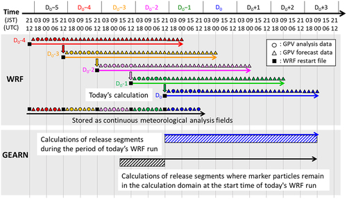
GSM-Japan datasets are distributed four times a day, which include analysis data at each initial time of 00, 06, 12, and 18 UTC (Coordinated Universal Time) and forecast data for the next 84 h with a time interval of 3 h for pressure levels and 1 h for the surface level. The boundary conditions used for the WRF calculation on a certain day in Japan Standard Time (JST, UTC +9 h), for example, D₀ in Figure 1, are created using five GSM-Japan datasets at the initial times of 12 and 18 UTC of 2 days before and 00, 06, and 12 UTC of the previous day. The WRF calculation on each day is executed using a restart file as the initial value, which is outputted by the calculation on the previous day and contains the calculation results 24 h after the start time of the calculation, so that the calculation is continuous. When the newest dataset (GSM-Japan data with the initial time of 12 UTC on the previous day in this example) is obtained, a WRF calculation for 4.5 days (1-day past analysis and 3.5-day forecast) is performed using these initial and boundary conditions. After the WRF calculation is complete, the following GEARN calculations are conducted:

1. Calculation using weather fields that have been updated and extended,

2. and recalculation of the release segment affecting the period for which the meteorological field was updated.

The former calculation is executed for release segments during the day’s WRF calculation period (blue shaded area in the lower GEARN part of Figure 1). The latter is executed for release segments where marker particles remain in the calculation domain at the start time of the day’s WRF calculation (i.e. 12 UTC on D₀ −2 in Figure 1) among the release segments calculated until the previous day (e.g. the black shaded area in the lower GEARN part of Figure 1). The number of such segments varies with each calculation. By automatically executing the above WRF and GEARN calculations every day, a continuous dispersion-DB from the past to several days ahead can be accumulated while updating the meteorological field with the latest input data.

2.3. Method of source term estimation and reconstruction of the spatiotemporal distribution of radionuclides

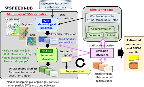
Figure 2 shows an overview of the source term estimation method and the reconstruction of the radionuclide spatiotemporal distribution using dispersion-DB produced by WSPEEDI-DB and environmental monitoring data.

Figure 2. Overview of the source term estimation method and reconstruction of the spatiotemporal distribution of radionuclides using WSPEEDI-DB and environmental monitoring data.

As in Terada et al. [13], the CO₂ emission estimation method [28] based on the Bayesian synthesis method [29] was used to estimate release rates by comparing ATDM simulation with environmental monitoring data. In this method, the hourly release rate vector (s) is estimated from the monitoring data vector (d) by minimizing the cost function (J) as follows:

(3) $\mathrm{J}=\left[{\left(\mathbf{M}\mathbf{s}-\mathbf{d}\right)}^{\mathrm{T}}\mathbf{C}{\left(\mathbf{d}\right)}^{-1}\left(\mathbf{M}\mathbf{s}-\mathbf{d}\right)+{\left(\mathbf{s}-{\mathbf{s}}_0\right)}^{\mathrm{T}}\mathbf{C}{\left({\mathbf{s}}_0\right)}^{-1}\left(\mathbf{s}-{\mathbf{s}}_0\right)\right]/2,$(3)

where M is the source receptor matrix for hourly release segments, which can be derived from the dispersion-DB described in Section 2.2, Ms corresponds to the calculated air concentration or deposition of radionuclides and hence Ms−d gives the difference between calculated and measured values; s₀ is the prior release rate vector; C(x) is the uncertainty covariance matrix for vector x [= σx(i)²δ(i, j)]; and δ is the Kronecker delta.

Settings of the diagonal components of C(x), uncertainty of each component of d and s₀ will be explained later in the description of the settings of each experiment. The solution for s to minimize J is given [30] below:

(4) $\mathbf{s}={\mathbf{s}}_0+{\left[{\mathbf{M}}^{\mathrm{T}}\mathbf{C}{\left(\mathbf{d}\right)}^{-1}\mathbf{M}+\mathbf{C}{\left({\mathbf{s}}_0\right)}^{-1}\right]}^{-1}{\mathbf{M}}^{\mathrm{T}}\mathbf{C}{\left(\mathbf{d}\right)}^{-1}\left(\mathbf{d}-\mathbf{M}{\mathbf{s}}_0\right).$(4)

In this method, matrix components from different dispersion-DB and monitoring data can be mixed in every single matrix of the source receptor matrix M and the monitoring data vector d, respectively. Based on this principle, we improved the release rate estimation code based on Bayesian inference. Thus, various monitoring data obtained in the vicinity to places far from the release point and multiple ATDM calculation results with different spatial scales ranging from local to hemisphere scales and different calculation periods are available to make the monitoring data vector and the source receptor matrix, respectively.

Environmental monitoring data of air concentration (Bq m⁻³), surface deposition (Bq m⁻²), and daily fallout (Bq m⁻² day⁻¹) are currently available for release rate estimation based on Bayesian inference. For air concentration, measurements at multiple points with an arbitrary temporal resolution and sampling period can be used, for example, continuous data at 1-h intervals and daily data. For surface deposition, horizontally distributed data derived by an airborne survey are assumed to be acquired. The data are used after being organized into mesh data using the averaged values on the calculation grid of ATDM. For daily fallout, deposition amounts measured at multiple discrete points every 24 h are used. Air dose rate data are not used for the release rate estimation in this study because a larger uncertainty is expected when the air dose rate is estimated from the calculated air concentration and the deposition of radionuclides using uncertain information of radionuclide composition for comparison with monitoring data.

2.4. Validation by application to the FDNPS accident

2.4.1. Dispersion-DBs

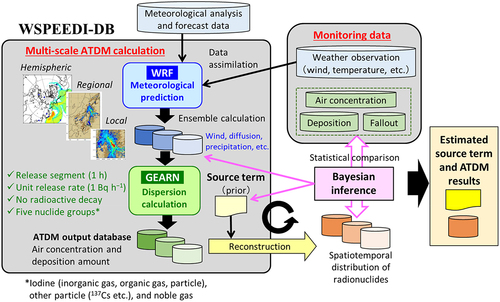
We used local- and regional-scale dispersion-DBs constructed in Terada et al. [13], which are briefly described as follows. Hereafter, dates and times are shown in JST. Calculation areas of local and regional dispersion-DB are 190 × 190 km² around the FDNPS, with a 1-km horizontal grid resolution (Domain 3 in Figure 3), and 570 × 570 km² in eastern Japan, with a 3-km horizontal grid resolution (Domain 2 in Figure 3), respectively. The meteorological calculation by WRF was conducted as a three-domain nesting calculation for Domains 1, 2, and 3 in Figure 3 using the Lambert conformal map projection. The dispersion calculation by GEARN was conducted as a two-domain nesting calculation for Domains 2 and 3. The calculation period is from 0:00 on March 12 to 0:00 on 1 April 2011. The GPV of the Meso-Scale Model, MSM, by JMA was used for the boundary and initial conditions of the WRF calculation. To improve the reproducibility of the meteorological fields, 4D-Var was applied for the calculation of Domain 1 using (1) wind observation data at the FDNPS, the Fukushima Daini nuclear power station (FD2NPS), and the Ohno monitoring post in the Fukushima Prefecture and (2) wind, air temperature, pressure, and relative humidity at the surface observation stations managed by JMA in the calculation domain. Additionally, the reproducibility of the meteorological fields was improved by combining ensemble meteorological calculations and Bayesian inference using ¹³⁷Cs SPM data [13]. Many members of dispersion-DBs were produced using meteorological fields with a slight difference by ensemble meteorological calculations. Then, with the Bayesian inference analysis using air concentrations calculated by each dispersion-DB and SPM data, the dispersion-DB indicating the lowest cost function was selected as the optimum meteorological case. The improvement of wind field mainly contributed to the improvement of reproducibility of plume movement. More details of the analysis are described in Terada et al. [13]. The detailed deposition scheme developed by Katata et al. [7] was used for local- and regional-scale GEARN calculations. The other calculation settings are summarized in Table 1.

Figure 3. Calculation domains for the local-, regional-, and hemispheric-scale dispersion-DBs. The colored shade in (a) indicates the topography height. The colored circles in (b) show the location of IMS-data monitoring points.

Table 1. Calculation settings for local- and regional-scale dispersion-DB.

Calculation domain	Domain 1	Domain 2	Domain 3
Horizontal grid resolution	9 km	3 km	1 km
Vertical grid of WRF	31 eta levels from surface to 100 hPa
Vertical grid of GEARN	29 z* levels from surface to 10 km with a 20 m-thick bottom layer
Time step of WRF	45 s	15 s	5 s
Time step of GEARN	-	12 s	4 s
Horizontal diffusion parameter in GEARN	Pasquil – Gifford chart (atmospheric stability: neutral)
Physical option of WRF
Land surface	Five-layer thermal diffusion [23]
Microphysics	WSM6 [31]
Cumulus	Betts – Miller–Janjic [32]		Not applied
Boundary layer	Mellor – Yamada–Nakanishi – Niino (MYNN) Level 2.5 [33]
Longwave radiation	Rapid Radiative Transfer Model (RRTM) [34]
Shortwave radiation	Dudhia [35]

We produced a hemispheric-scale dispersion-DB with the same settings as those used in [14], except for the calculation period. Brief descriptions are as follows. The calculation area (Figure 3) is 16,500 × 16,500 km², with a 54-km horizontal grid resolution. The polar stereographic projection was used by centering at the North Pole. The calculation period is from 0:00 on March 12 to 0:00 on 21 April 2011, which is extended compared to that in Kadowaki et al. [14] to consider the effect of the hemispheric atmospheric dispersion on the source term estimation during a period longer than that of the regional dispersion. The simple conventional deposition scheme [27] was used for hemispheric-scale GEARN calculations. The other calculation settings are summarized in Table 2.

Table 2. Calculation settings for the hemispheric-scale dispersion-DB.

Horizontal grid resolution	54 km
Vertical grid of WRF	31 eta levels from surface to 100 hPa
Vertical grid of GEARN	29 levels from surface to 10 km with a 20 m-thick bottom layer
Time step of WRF	60 s
Time step of GEARN	30 s
Horizontal diffusion parameter in GEARN	Gifford (1982) scheme [25] modified by Terada et al [26].
Initial and boundary condition of WRF	GPV of GSM by JMA
Data assimilation in WRF	Analysis nudging with the GPV
Physical option of WRF
Land surface	Five-layer thermal diffusion [23]
Microphysics	Morrison double-moment scheme [36]
Cumulus	Betts – Miller–Janjic [32]
Boundary layer	Mellor – Yamada–Nakanishi – Niino (MYNN) Level 2.5 [33]
Longwave radiation	Rapid Radiative Transfer Model (RRTM) [34]
Shortwave radiation	Dudhia [35]

As common settings for all the dispersion-DB, the time intervals of release segment and dispersion-calculation outputs were set as 1 h. The dispersion-DB was created for four release height cases: point sources of 20 m and 120 m above the ground and volume sources with 100 × 100 × 100 m³ and 100 × 100 × 300 m³ (length in x-, y-, and z-directions, respectively) for hydrogen explosions at Units 1 and 3, respectively.

2.4.2. Environmental monitoring data

The various data of air concentration, surface deposition, and daily fallout data shown in Table 3 were used in this study. For estimation of the release rate of ¹³⁷Cs using the local- and regional-scale dispersion-DB, we used the dust sampling data (47 points) [37–44], SPM data (100 points) [46,47], the surface deposition map generated by the airborne survey [54], and the daily fallout data (13 points) [55] that were used in a previous study [13]. In this study, dust sampling data in Tokyo (1 point) [45] and NaI data at monitoring stations in the Ibaraki Prefecture (6 points) [48,49] were also used. For the SPM data, 6-h average values for the periods partitioned with the start time at 0:00 were used for the estimation to reduce discrepancies caused by temporal deviation of the calculated plume passage at the monitoring points in the same way as those in [13]. In the validation of ¹³⁷Cs air concentration of the dispersion-DB used in this study, 6-h average values were evaluated to have a required reproducibility for the public dose evaluation conducted at 6-h intervals. The SPM data at the Futaba monitoring point (Figure 3a) were not used because the location is in the FDNPS vicinity (3.2 km west-northwest), and the spatial resolution of even local-scale dispersion-DB (1 km) is not enough to simulate the air concentration at the point. However, the data were used to consider the prior release rate described later in Section 2.4.3. For the estimation using the hemispheric-scale dispersion-DB, we used the global-scale air concentration data measured at the stations of the International Monitoring System (hereafter: IMS data), which is a part of the verification system of the Comprehensive Nuclear-Test-Ban Treaty Organization (CTBTO) (24 points) [50]. The dust sampling data in Europe (170 points) [51], Seattle in the USA (1 point) [52], and Taiwan and Tibet (5 points) [53] were also used. The components of the uncertainty covariance matrix for the monitoring data $\mathbf{C}\left(\mathbf{d}\right)$ were set for each data type based on their standard deviations. For the SPM and IMS data, the standard deviation was calculated at each measurement point. For other data, one fixed value was set (deposition data: 300,000 Bq m⁻²; fallout data: 1,000 Bq m⁻² day⁻¹; domestic dust sampling and NaI data: 70 Bq m⁻³, dust sampling data in Europe: 1 × 10⁻⁴ Bq m⁻³; dust sampling data in Taiwan and Tibet: 7 × 10⁻⁴ Bq m⁻³; dust sampling data in the USA: 2 × 10⁻⁴ Bq m⁻³).

Table 3. Environmental monitoring data used by the source term estimation in the present study. ‘Dust’ means air concentration data from dust sampling.

Data	Spatial characteristic	Temporal characteristic (time interval)
Air concentration (domestic)
Dust in Fukushima Prefecture [37]	Several points	Specific time
Dust near FDNPS [38]	Several points	Specific time
Dust at FD2NPS [39]	A point	Mostly daily
Dust at JCAC [40]	A point	Mostly daily
Dust at JAEA-1 [41]	A point	Time series (fluctuate)
Dust at JAEA-2 [42]	A point	Time series (fluctuate)
Dust at JAEA-3 [43]	A point	Time series (fluctuate)
Dust at KEK [44]	A point	Mostly daily
Dust in Tokyo [45]	A point	Time series (fluctuate)
SPM data [46,47]	Many points	Time series (1 h)
NaI data [48,49]	Several points	Time series (1 h)
Air concentration (overseas)
IMS data [50]	Many points	Mostly daily
Dust in Europe [51]	Many points	Mostly daily
Dust in USA [52]	A point	Mostly daily
Dust in Taiwan and Tibet [53]	Several points	Mostly daily
Surface deposition amount (domestic)
Airborne survey data [54]	Map (mesh data)	Specific time
Fallout (domestic)
Daily fallout data [55]	Several points	Daily

The uncertainty of the dispersion calculation was added to $\mathbf{C}\left(\mathbf{d}\right)$, as shown in Terada et al. [13]. The uncertainty of the calculated value at the monitoring point and each time segment was obtained from the sum of the absolute difference values between the grid of the monitoring point and the four points surrounding it divided by the average value of the five points. Subsequently, this value was multiplied by the component value of $\mathbf{C}\left(\mathbf{d}\right)$ at the monitoring point.

For validation, surface deposition calculated by applying the source term to regional-scale dispersion-DB was compared with airborne monitoring data. Air concentrations calculated by local- and regional-scale dispersion-DBs were compared with the SPM data, and those by hemispheric-scale dispersion-DB were compared with the IMS data. The validations in this study are intended to evaluate the extent to which one of the most important monitoring data in the data used for the estimation can be reproduced when the release rate is estimated using multiple data including the data used for the validations. A cross-validation is not conducted because optimization of the Bayesian estimation code (model) by parameter fitting, etc., using the measurement data as training data is not performed in this study.

2.4.3. Sensitivity experiment of release rate estimation using various monitoring data

To evaluate the effects of each monitoring data on source term estimation, we conducted estimation experiments of ¹³⁷Cs release rate using different monitoring data and dispersion-DBs (Table 4). In the ALL case, all the domestic and overseas environmental monitoring data were used with the local-, regional-, and hemispheric-scale dispersion-DBs. In the other cases, limited monitoring data were used, as shown in Table 4, and only the local- and regional-scale dispersion-DB were used. In the DST case, only the domestic dust sampling data that are temporally and spatially discrete were used. In the CON case, SPM and NaI domestic air concentration data, which were the multipoint continuous data, were added to the DST case. In the DEP case, only the deposition map data of derived by the airborne monitoring and daily fallout data in Japan were used. In the DOM case, all the domestic data, including air concentration and deposition, were used.

Table 4. Cases in the sensitivity experiment of release rate estimation.

Case	Characteristic	Used monitoring data in Table 3	Used dispersion-DB
DST	Use of spatiotemporally scattered domestic air concentration data	Air concentration (domestic) without the SPM and NaI data	Local and regional DB
CON	Use of domestic air concentration data with continuous data at many points	Air concentration (domestic)	Local and regional DB
DEP	Use of only deposition data	Airborne survey data and daily fallout data	Local and regional DB
DOM	Use of domestic air concentration and deposition data	Air concentration (domestic), airborne survey data, and daily fallout data	Local and regional DB
ALL	Use of all the domestic and overseas data	Air concentration (domestic), air concentration (overseas), airborne survey data, and daily fallout data	Local, regional, and hemispheric DB

In the previous study [13], the hourly release rate values generated from the source term estimated by Katata et al. [7], with modifications for some periods based on the results from Chino et al. [8], were used as the prior release rate for the release rate estimation based on the Bayesian inference. In the present study, we additionally modified the release rate for a part of the period by comparing the analytical calculation results of atmospheric dispersion by a Gaussian plume model with the measured ¹³⁷Cs air concentration of SPM data at the Futaba Station [47]. The nine plume arrivals (p1, p1 v, P1,’ P3, P5, P6, P8, P10, and P11) were highlighted from the measured ¹³⁷Cs air concentrations at the Futaba Station by Tsuruta et al. [47]. Afterward, we reversely estimated the release rates of the nine plumes by comparing the maximum values of the measured ¹³⁷Cs air concentrations with the Gaussian model calculation results [56] under the conditions of wind speed of 1 m s⁻¹ and unit release rate (10⁹ Bq h⁻¹). Among the nine plumes, we adopted the release rate estimated by this method during the latter peak period of the P3 plume (20:00–21:00 on March 15) when the uncertainty of the estimated release rate using the air dose rate in Katata et al. [7] was considered relatively large. The previous release rate of 7.6 × 10¹³ Bq h⁻¹ was modified to 4.2 × 10¹² Bq h⁻¹ for ¹³⁷Cs (decay corrected at the shutdown time). The estimated release rates for the plumes other than P3 were not used because the plume centers did not pass over the Futaba Station due to the large discrepancies between the direction of the Futaba Station from FDNPS (west-northwest) and the wind directions measured at FDNPS or FD2NPS. The uncertainty covariance matrix for the prior release rate C (s₀) was generated assuming that the release rate at each time segment had 100% uncertainty, as σs₀ (i) = s₀ (i) in this experiment.

2.4.4. Experiment of real-time source term estimation

To validate the real-time application of the source term estimation method, we conducted an estimation experiment of ¹³⁷Cs release rate using a scenario of environmental monitoring data acquisition after the FDNPS accident. In the experiment, a three-step release rate estimation was conducted using the increasing environmental monitoring data available at three time points after the accident – Phase-1: 2 days after (March 13); Phase-2: 1 week after (March 17); and Phase-3: 3 weeks after (March 31). Environmental monitoring data used at each phase are shown in Figure 4.

Figure 4. Environmental monitoring data used in the real-time source term estimation experiment.

In this experiment, we conducted the source term estimations using only the local- and regional-scale dispersion-DBs and the domestic monitoring data described in Section 2.4.2. It is important to respond as quickly as possible in an emergency situation. Since it takes a long time for the analysis using a long-term hemispheric-scale dispersion-DB, and it is unclear when the global dataset can be obtained due to the situation of countries where the measurements are conducted, overseas monitoring data and the hemispheric-scale dispersion-DB were not included in this experiment.

Although SPM data, NaI data, and the surface deposition map derived by airborne monitoring were not actually obtained within 3 weeks (Phase-3) but rather several months or years after the accident, they were assumed to be acquired in a technically feasible time. For the release start time, 5:00 on March 12, as same as that of the prior source term described in Section 2.4.3, was used assuming that it can be estimated from measured air dose rates at onsite monitoring posts and plant parameters. Release height is also assumed to be a known parameter in this experiment, as it is expected to be set from plant events, such as explosions, smoke from stacks or buildings.

The procedure of the three-step source term estimation for the real-time estimation experiment and the feature of environmental monitoring data used in each phase is as follows:

• Phase-1: The estimation was done using monitoring data that were available until March 13 with the prior release rates of constant and continuous rates of 10¹³ Bq h⁻¹. Only the air concentration data in Fukushima Prefecture were used.

• Phase-2: The prior release rates (where the release rates from March 12 to March 13 were set from the results at Phase-1 and those from March 14 to March 17 were kept constant at 10¹³ Bq h⁻¹) were modified using monitoring data that were available until March 17. Air concentration data in areas outside Fukushima Prefecture were added.

• Phase-3: The prior release rates (where the release rates from March 12 to March 17 were set from the results at Phase-2, and those from March 18 to March 31 were kept constant at 10¹³ Bq h⁻¹) were modified using monitoring data that were available until March 31. Deposition data (daily fallout and deposition map) were added.

The uncertainty of the prior release rate in the source term estimation was set as 10-time values of the prior release rates, as σs₀ (i) = 10 s₀ (i), because the prior release rate is an assumed value based on the estimated source term of the FDNPS accident and is expected to have a larger uncertainty. For other uncertainties, we used the same settings as those described in Section 2.4.2. When estimated release rates become negative values, these values were corrected to 10¹⁰ Bq h⁻¹ as a minimum release rate.

The specifications of the computer used for the release rate estimation in this study are as follows: Intel® Xeon® G 6136 CPU (3.0 GHz), with 24 cores and 96 GB memory. The source term estimation code is not parallelized.

3. Results and discussion

3.1. Effects of various environmental monitoring data on the source term estimation

The temporal variations of the release rates by the sensitivity experiment described in Section 2.4.3 are shown in Figure 5. The hourly release rates that were estimated by the Bayesian inference method were averaged for each release segment with a constant value in the prior release rate in the same way as in Terada et al. [13]. The air concentration and surface deposition of ¹³⁷Cs calculated by application of the averaged release rates to the dispersion-DBs were compared with the measurements. The statistical comparison results of 6-h average values of the ¹³⁷Cs air concentrations calculated using regional- and local-scale dispersion-DBs with the SPM data are shown in Table 5. The surface deposition distributions of ¹³⁷Cs calculated by the averaged estimation results of the release rates are shown in Figure 6. The statistical comparison results of the ¹³⁷Cs surface deposition with the measurement by the airborne survey are summarized in Table 6.

Figure 5. Estimation results of ¹³⁷Cs release rates in the sensitivity experiment.

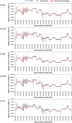
Figure 6. Comparison of the calculated distributions of ¹³⁷Cs surface deposition in the sensitivity experiment.

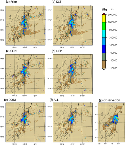
Table 5. Statistics of the comparison of 6-h average values of ¹³⁷Cs air concentration between calculations by each case in the sensitivity experiment of release rate estimation and SPM data; the ratio of the calculations within factors of 2, 5, and 10 of the measurements (FA2, FA5, FA10, respectively), logarithmic correlation coefficient (CC_log), fractional bias (FB), normalized mean square error (NMSE), and the number of compared pairs of values (n) with a minimum cutoff for the measured values: 1 Bq m⁻³.

Case	FA2	FA5	FA10	CClog	FB	NMSE	n
Prior	0.20	0.41	0.49	0.57	0.76	57.6	459
DST	0.20	0.41	0.49	0.58	0.76	57.0	459
CON	0.20	0.39	0.46	0.61	0.41	43.7	459
DEP	0.18	0.39	0.48	0.57	0.42	48.6	459
DOM	0.19	0.38	0.46	0.61	0.23	37.0	459
ALL	0.20	0.39	0.47	0.61	0.11	37.6	459

Table 6. Statistics of the comparison of ¹³⁷Cs surface deposition between regional-scale calculations by each case in the sensitivity experiment of release rate estimation and airborne survey data; FA2, FA5, FA10, correlation coefficient (CC), FB, NMSE, and the number of compared pairs of values (n) with a minimum cutoff: 10 Bq m⁻².

Case	FA2	FA5	FA10	CC	FB	NMSE	n
Prior	0.33	0.67	0.82	0.72	−0.10	9.2	3518
DST	0.33	0.67	0.82	0.72	−0.10	9.2	3516
CON	0.37	0.68	0.81	0.76	−0.23	8.1	3507
DEP	0.36	0.67	0.81	0.78	−0.25	8.1	3516
DOM	0.37	0.67	0.81	0.79	−0.30	7.9	3506
ALL	0.38	0.68	0.81	0.80	−0.32	7.7	3508

3.1.1. Effect of use of spatially and temporally dense data

The estimated release rates in the DST, CON, and DEP cases were compared with the prior release rate focusing on the change of the release rate greater than 30% of the prior one (this criterion is used in subsequent comparisons of release rates). In the DST case (Figure 5a), the release rate was modified within limited periods: the decreases from 5:00 to 9:00 on March 12, 21:00 to 22:00 on March 15, and 16:00 to 21:00 on March 21 and the increases from 3:00 to 4:00 and 20:00 to 21:00 on March 15. This is because most of the dust sampling data used in this case has already been used in estimating the prior release rates. In the CON case (Figure 5b), additional SPM data affected the release rate for more periods in addition to that of the DST case: the decreases from 5:00 to 9:00 and 14:00 to 16:00 on March 12, 23:00 on March 14 to 2:00 on March 15, 21:00 on March 15 to 1:00 on March 16, 5:00 on March 18 to 15:00 on March 19, 10:00 on March 20 to 8:00 on March 21, and 16:00 to 21:00 on March 21 and the increases from 21:00 to 22:00 on March 14, 2:00 to 4:00 and 20:00 to 21:00 on March 15. In the DEP case, the release rate was modified by additional deposition measurement data in the following periods: the decrease from 14:00 to 16:00 on March 12, 7:00 to 10:00 on March 15, 21:00 on March 15 to 1:00 on March 16, and 10:00 on March 20 to 8:00 on March 21 and the increases from 16:00 to 18:00 and 20:00 to 21:00 on March 15.

The reproducibility of the dispersion-calculation results using the estimated release rate in each case is compared. In the statistical comparison of ¹³⁷Cs air concentrations with the SPM data (Table 5), no major changes in statistical scores are seen in the DST case compared with the results by the prior release rate (hereafter: the ‘Prior’ case). In contrast, the CON case shows better scores than the Prior case (CC_log increased from 0.57 to 0.61, FB decreased from 0.76 to 0.41, and NMSE decreased from 57.6 to 43.7). Furthermore, the DEP case also shows better scores than the Prior case in the comparison of air concentrations (FB decreased from 0.76 to 0.42 and NMSE decreased from 57.6 to 48.6), even though air concentration measurement data are not used in the release rate estimation.

The reproducibility of ¹³⁷Cs surface deposition is evaluated by comparing the horizontal distributions (Figure 6) and statistical analysis (Table 6) with the measurement data derived by an airborne survey. Compared with the deposition distribution in the Prior case (Figure 6a), no particular difference is seen in that in the DST case (Figure 6b). Conversely, overestimation over the southeast coastal area of the Ibaraki Prefecture in the Prior case is reduced in the CON and DEP cases. Moreover, underestimation around the north of the Tochigi and Gunma Prefectures in the Prior case is mitigated in the CON case, where the measured deposition data are not used in estimating the release rate. In the CON case, the release rates increased compared to the Prior case in the following three periods: (1) 21:00 to 22:00 on March 14, (2) 2:00 to 4:00 on March 15, and (3) 20:00 to 21:00 on March 15. From the comparison among the simulated increases of ¹³⁷Cs deposition distribution created by applying only each increase in the release rate of (1) to (3) to the regional-scale dispersion-DB (not shown in the figures), it was indicated that the increase of the release rate in the period: (2) 2:00 to 4:00 on March 15 contributed to the above improvement in the deposition distribution.

In the statistical comparison of surface deposition (Table 6), no difference was seen between the results in the Prior and DST cases. Both CON and DEP cases show better statistical scores than the Prior case. FA2 increased to 0.37 in the CON case and 0.36 in the DEP case from 0.33 in the Prior case. CC increased to 0.76 in the CON case and 0.78 in the DEP case from 0.72 in the Prior case. NMSE decreased to 8.1 in the CON and DEP cases from 9.2 in the Prior case. Conversely, the CON and DEP cases demonstrated lower scores in FB (−0.23 and −0.25, respectively) than the Prior case (−0.10). This may be attributed to the modification of release rates to improve the overestimation of air concentrations shown by an FB of 0.76 in the Prior case (Table 5). However, the decrease of FB for deposition from the Prior case to the CON case (0.13, from −0.10 to −0.23) is smaller than that for air concentrations (0.35, from 0.76 to 0.41), indicating that the release rate is comprehensively optimized based on the reproducibility of both concentration and deposition.

These results suggest that multipoint continuous data, such as SPM data, and distribution-type data, such as the surface deposition map derived by the airborne survey, have a greater impact on release rate estimation than discrete data, such as dust sampling data. In addition, it was shown that estimation of release rates using either air concentration or deposition monitoring data with a high spatial and temporal resolution improves the reproducibility of the others.

3.1.2. Effect of concurrent use of air concentration and deposition data

To evaluate the effects of using both air concentration and surface deposition data compared to using only one of them, the estimation results in the DOM case were compared with those in the CON and DEP cases.

In the DOM case (Figure 5d), the release rates decreased from 5:00 to 9:00 and 14:00 to 16:00 on March 12, 23:00 to 24:00 on March 14, 1:00 to 2:00 and 7:00 to 10:00 on March 15, 21:00 on March 15 to 1:00 on March 16, 5:00 to 18:00 on March 18, 10:00 on March 20 to 8:00 on March 21, and 16:00 on March 21 to 0:00 on March 24 and conversely increased from 21:00 to 22:00 on March 14 and 2:00 to 4:00, 16:00 to 18:00, and 20:00 to 21:00 on March 15. This result shows a combined feature of both effects on the CON and DEP cases.

In the statistical comparison of ¹³⁷Cs air concentrations with the SPM data (Table 5), better statistical scores are shown in the DOM case compared with the CON and DEP cases (for example, FB decreased from 0.41 to 0.23 and NMSE decreased from 43.7 to 37.0). From the comparison of the surface deposition distributions among the CON (Figure 6c), DEP (Figure 6d) and DOM (Figure 6e) cases, it can be seen that the overestimation of the southeast coastal area of the Ibaraki Prefecture in the CON and DEP cases has improved in the DOM case while maintaining the high deposition areas in the Tochigi and Gunma Prefectures calculated in the CON case. From the statistical comparison of surface deposition (Table 6), the DOM case shows better statistical scores (CC: 0.79 and NMSE: 7.9) compared with the CON (CC: 0.76 and NMSE: 8.1) and DEP (CC: 0.78 and NMSE: 8.1) cases, although FB decreased to −0.30 in the DOM case from −0.23 in the CON case and −0.25 in the DEP case in association with the decrease of FB for the air concentration in the DOM case (Table 5). The above results quantitatively demonstrate how much more effectively the release rates are optimized when using both air concentration and surface deposition measurement data than when using either one.

3.1.3. Effect of use of hemispheric-scale data in addition to local- and regional-scale data

In the ALL case (Figure 5e), the release rates decreased over more periods than in the previously described cases. As same as the DOM case, the periods when the release rates decreased in the ALL cases are from 22:00 on March 12 to 3:00 on March 14, 9:00 to 11:00 on March 16, 13:00 on March 16 to 6:00 on March 17, and from 18:00 on March 18 to 15:00 on March 19. Because the temporal and spatial distributions of measured data vary depending on the environmental monitoring data shown in Table 3, the release time when the Bayesian estimation affects varies according to the data used. In the ALL case, the most data were used, then release rates were changed at the release times that were not affected in other cases.

In the statistical comparison of ¹³⁷Cs air concentrations with the SPM data (Table 5), statistical scores in the ALL case show little difference from the DOM case except for the decrease of FB from 0.23 to 0.11. From the comparison of the spatial distribution (Figure 6) and statistical scores of ¹³⁷Cs surface deposition (Table 6), almost no difference was seen between the ALL case and the DOM case. This is because the overseas environmental monitoring data, which were additionally used in the ALL case, have less impact on the domestic deposition distribution compared with the domestic environmental monitoring data.

In the ALL case, hemispheric-scale dispersion-DB and overseas monitoring data of air concentrations are additionally used in the release rate estimation based on Bayesian inference. To evaluate the effect of using the hemispheric data on the estimation, air concentrations calculated by applying release rates estimated in the Prior, DOM, and ALL cases to the hemispheric-scale dispersion-DB were compared statistically with the IMS data (Table 7). The statistical indicator BIAS was calculated as follows:

(5) $\mathrm{B}\mathrm{I}\mathrm{A}\mathrm{S}=\frac{1}{n}\sum {log}_{10}\left(\frac{CAL}{OBS}\right)$(5)

Table 7. Statistics of the comparison of daily average values of ¹³⁷Cs air concentration between hemispheric-scale calculations by three cases in the sensitivity experiment of release rate estimation and IMS data; FA10, BIAS, and the number of compared pairs of values (n). Statistics were calculated for fractions of samples at specific sites (Pacific and Other in Fig. 3b) and all sites (Total) with a minimum cutoff: 10⁻⁶ Bq m⁻³.

Compared monitoring site	Case	FA10	BIAS	n
Total	Prior	0.70	0.36	244
	DOM	0.73	0.21	242
	ALL	0.78	0.03	236
Pacific	Prior	0.67	0.44	190
	DOM	0.71	0.30	188
	ALL	0.77	0.10	185
Other	Prior	0.81	0.09	54
	DOM	0.81	−0.09	54
	ALL	0.80	−0.25	51

where CAL and OBS are the calculated and measurement values, respectively, and n is the total number of pairs for the values compared. From the statistical comparison for all the monitoring sites (‘Total’ in Table 7), the statistical scores in the ALL case show the best scores (FA10 = 0.78 and BIAS = 0.03) compared with those in the Prior and DOM cases. The comparison of only ‘Pacific’ monitoring sites (Figure 3b) also shows better statistical scores in the ALL case (FA10 = 0.77 and BIAS = 0.10) than in the DOM and Prior cases. However, when comparing monitoring sites other than the Pacific sites (‘Other’ in Table 7), the ALL case shows a considerable underestimation compared to the DOM case (BIAS = −0.25).

In the previous study where the hemispheric-scale dispersion-DB used in this study was produced, it was reported that the air concentrations in the dispersion-DB are overestimated due to underestimation of deposition calculations caused by poor reproducibility of precipitation in the Pacific region [14]. Subsequently, the estimation in the ALL case using this dispersion-DB and only the air concentration measurement data caused a downward adjustment of the release rates so that the overestimated air concentrations could be adjusted to the measured values in the Pacific region. This decreased release rate resulted in the underestimation of air concentrations at ‘Other’ sites where the air concentrations were affected by precipitation scavenging in the Pacific region on the dispersion pathway from the FDNPS. This result suggests that reproducing both air concentrations and surface deposition using ATDM or both measurements is important to estimate the source term properly.

For detailed analysis in the medium to long term after an accident, a comparison of dispersion calculations on the hemispheric, local, and regional scales with the measurement is effective for improving the accuracy of the estimated source term. However, monitoring fallout from the atmosphere over the ocean is difficult. Therefore, if the dispersion pathway of radionuclides includes the ocean, evaluating the prediction performance of ATDM for both air concentration and deposition is important to properly estimate source terms using measured air concentrations at a distance. As an advanced method, source terms can be estimated by comparing ocean monitoring data with oceanic dispersion simulation using the amount of fallout to the sea from ATDM as input. However, it should be noted that this will increase the uncertainty mainly due to the approximation of physical processes in the oceanic dispersion simulations and temporal and spatial representativeness of the monitoring data.

3.2. Validity of real-time source term estimation

The temporal variations of the release rates by the real-time source term estimation experiment described in section 2.4.4 are shown in Figure 7. The estimated result of Phase-1 (Figure 7a) shows a decrease in release rates from the initial release rate from 5:00 to 9:00 on March 12 and increases from 10:00 to 11:00 and 12:00 to 14:00 on March 12 and 2:00 to 3:00 on March 13. This variation in the release rate which is low in the morning of March 12 and increases in the afternoon corresponds to the estimation results in the DOM case using all the domestic data described in Section 3.1. In the Phase-2 results (Figure 7b), this release rate variation on March 12 is more prominent, with an estimated increase of over 10¹⁴ Bq h⁻¹ from 14:00 to 16:00 on March 12. In the subsequent period, increases in the release rates are estimated from 20:00 on March 14 to 13:00 on March 15. In addition to the variations on March 12 similar to the Phase-1 results, several increases from the night of March 14 to early morning of March 15 estimated in the Phase-2 results correspond to the DOM case results. The increases in the afternoon of March 15 and March 16, which are estimated in the DOM case, are not estimated in the Phase-2 results. This can be attributed to the effect that no deposition data were used in the Phase-2. The final estimation results of Phase-3 (Figure 7c) show a further increase from 15:00 to 16:00 on March 12, with additional increases from afternoon to evening on March 15, in the morning on March 16, from March 18 to March 21, and on March 31. Comparing the characteristics of this variation in the release rates in the Phase-3 with the estimation results in the DOM case, a good correspondence is seen between the two results.

Figure 7. Temporal variations of the release rates estimated in the real-time source term estimation experiment.

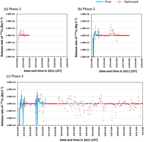
The total release amount of ¹³⁷Cs from March 12 to 31 of the Phase-3 results is 8.3 PBq, which is calculated by accumulating the release rates that are temporally averaged with the same method described in Section 3.1 as used for the sensitivity experiment. This amount is 16% less than the total release amount of 9.9 PBq calculated from the estimated result in the DOM case of the sensitivity experiment. However, this estimate is useful in assessing the approximate scale of the accident 3 weeks later.

To evaluate the improvement of accuracy in the source term by the stepwise estimation of release rate in Phase-1 to Phase-3, the dispersion calculation results from March 12 to 31 using the estimated release rates were compared with the measurement data. The release rates used for the dispersion calculation from March 12 to 31 were created using the estimated release rates for the estimation period of each phase and the initial release rate (10¹³ Bq h⁻¹, constant) for the period after the estimation period in each phase until March 31. By applying the release rates to the local- and regional-scale dispersion-DB, hourly ¹³⁷Cs air concentration and accumulated surface deposition were calculated for March 12 to 31.

Table 8 shows the results of statistical comparisons between ¹³⁷Cs air concentrations calculated by the initial and estimated release rates in each phase and SPM data. The Phase-1 results show no significant change in statistical scores compared to the results using the initial release rate (hereafter: ‘Initial’) except for NMSE, but the Phase-2 results show significant improvement for all statistical scores. In Phase-3, only FB changed greatly from −0.14 in Phase-2 to 0.01 in Phase 3, showing almost no bias.

Table 8. Statistics of the comparison of 6-h average values of ¹³⁷Cs air concentration between calculations by each phase in the experiment of real-time source term estimation and SPM data; FA2, FA5, FA10, CC_log, FB, NMSE, and the number of compared pairs of values (n) with a minimum cutoff for the measured values: 1 Bq m⁻³.

	FA2	FA5	FA10	CClog	FB	NMSE	n
Initial	0.07	0.24	0.36	0.55	−0.69	100.4	459
Phase-1	0.08	0.24	0.36	0.56	−0.64	94.3	459
Phase-2	0.19	0.38	0.46	0.59	−0.14	25.5	459
Phase-3	0.21	0.39	0.46	0.61	0.01	24.7	459

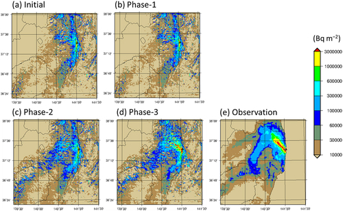
The regional- and local-scale distributions of accumulated ¹³⁷Cs surface deposition until March 31 calculated by using the initial and estimated release rates in Phase-1, 2, and 3 are shown in Figures 8 and 9, respectively. The calculation results in Phase-1 (Figure 8b and Figure 9b) show almost no change from the Initial results. In Phase-2 (Figure 8c and 9c), although the area with a high deposition amount near FDNPS in the measurements (Figure 6g and 9e) was not calculated, the areas with a high deposition amount in the central Fukushima Prefecture, northern Tochigi and Gunma Prefectures, and southern Ibaraki Prefecture are well calculated. In addition to this deposition distribution, the area with a high deposition amount extending in a northwest direction near the FDNPS area is well reproduced in Phase-3 (Figure 8d and 9d).

Figure 8. Comparison of the calculated regional-scale distributions of ¹³⁷Cs surface deposition in the real-time source term estimation experiment.

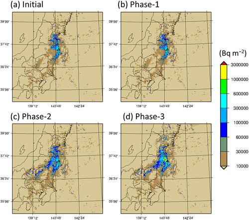
Figure 9. Comparison of the calculated local-scale distributions of ¹³⁷Cs surface deposition in the real-time source term estimation experiment.

Table 9 shows the statistical comparison of the regional-scale ¹³⁷Cs depositions. As with the comparison of air concentrations, Phase-1 shows little change in all the statistical scores from the Initial. In Phase-2, the statistical scores improved (for example, FA5 increased from 0.61 to 0.78, FB increased from −0.96 to −0.6, and NMSE decreased from 33.8 to 21.2), except for CC_log, even though the deposition and fallout measurements were not used in the release rate estimation. In Phase-3, all the statistical scores show more improvements than in Phase-2 (CC_log increased from 0.50 to 0.84, FB increased from −0.6 to −0.14, and NMSE decreased from 21.2 to 5.0).

Table 9. Statistics of the comparison of ¹³⁷Cs surface deposition between regional-scale calculations by each phase in the experiment of real-time source term estimation and airborne survey data; FA2, FA5, FA10, CC_log, FB, NMSE, and the number of compared pairs of values (n) with a minimum cutoff: 10 Bq m⁻².

	FA2	FA5	FA10	CClog	FB	NMSE	n
Initial	0.30	0.61	0.78	0.54	−0.97	34.0	3521
Phase-1	0.30	0.61	0.78	0.53	−0.96	33.8	3521
Phase-2	0.44	0.78	0.88	0.50	−0.60	21.2	3522
Phase-3	0.47	0.81	0.90	0.84	−0.14	5.0	3522

The above results suggest the following:

• If an ATDM can reconstruct both air concentrations and surface deposition with high accuracy, it is possible to estimate source terms that can be used to understand the overview of surface contamination (deposition distribution) even in the early stage of an accident when air concentration measurements are available, but those of deposition and fallout are difficult to obtain.

• Once deposition and air concentration measurement data are obtained, the accuracy of the estimated source term and reproducibility of the dispersion-calculation results using the source term increase remarkably.

• The total amount of released radionuclides calculated from the source term, which is estimated using the monitoring data acquired when most of the major release has been completed and major surface contamination has been formed, provides reference information sufficient to evaluate the approximate scale of the accident.

The time required to estimate the release rate is an important factor in emergencies. In the real-time source term estimation experiment, the time to estimate the release rate using the Bayesian inference method was 1 min 28 s for Phase-1, 4 min 3 s for Phase-2, and 18 min 9 s for-Phase 3. These analysis times do not include the time required for atmospheric dispersion calculations to create the dispersion-DB. However, as described in Section 2.2, past dispersion-DBs can be continuously stored by automatically executing meteorological and dispersion calculations using WSPEEDI-DB following updates of meteorological forecast and analysis data, which are distributed several times daily.

The results of this study indicate that the multipoint continuous data of measured air concentrations (such as SPM and NaI data) and distribution-type data of measured surface deposition (such as the deposition map by an airborne survey) are highly important for accurate source term estimation. Although it is difficult to obtain such data in real time at this point, deployment of continuous measurement equipment for air concentrations in the areas surrounding nuclear facilities and enhancement of the airborne survey technology are underway in Japan for normal and emergency monitoring since the FDNPS accident. Therefore, assuming that the environmental monitoring data used in this study can be obtained online with a common data format in near real time, this source term estimation method makes it possible to obtain source terms useful for emergency responses immediately (e.g. within a few to several tens of minutes after acquiring the environmental measurement data). In addition, it would be preferable to take into account when and how much reliable source term and dispersion calculation results need to be obtained in the planning of the development of this monitoring framework; the results of this study are useful as reference information for the consideration.

Air dose rate data, which are not used in this study, are expected to be available in real time with temporally and spatially dense distributions in the vicinity of nuclear facilities. Therefore, these data will be highly effective in this source term estimation method. However, when using the air dose rate, the nuclide composition ratio is necessary, and the physicochemical properties of the target nuclides, such as chemical forms and particle size for particulate form, may affect the reproducibility in ATDM calculations. For proper consideration of this information, it will be important to consider coordination with severe accident progression analysis and the use of information from environmental monitoring. In addition, to use the monitoring data at the vicinity of the release point in the source term estimation based on the Bayesian inference method, the ATDM calculations with higher spatial resolution than that in this study will need to be validated. It would be also worthwhile to consider the combination use with other ATDM using large-eddy simulation [57,58].

The initial release rate and setting of its uncertainty, such as the magnitude and function form, have a large impact on its estimation results by the source term estimation method based on Bayesian inference used in this study. This issue needs to be further studied when this source term estimation method is implemented in a real-time system in the future. Although the initial release rate was assumed constant in this study, it will be possible to reduce its uncertainty when information such as particle size, chemical form, and approximate release amount of released radionuclides according to scenario and magnitude of accidents is acquired from study of severe accident progression analysis.

Furthermore, the reproducibility of the meteorological field used for ATDM calculations, which was not tackled in this study, is a factor that considerably impacts on source term estimation and reconstruction of the environmental distribution of radionuclides. To reduce the uncertainty of the analysis results, improving the reproducibility of the dispersion calculation by regularly updating the dispersion-DB through data assimilation using various meteorological observation data acquired in real time and a coupled analysis of the ensemble calculation and the Bayesian inference method as implemented in Terada et al. [13] is effective. In relation to the uncertainty due to the meteorological field, a study is in progress to evaluate the uncertainty of atmospheric dispersion forecasts due to meteorological fields using the dispersion-DB created by WSPEEDI-DB [59]. By combining it with the source term estimation method presented in the present study, quantitative atmospheric dispersion forecasts can be presented together with uncertainty information.

4. Conclusions

We evaluated the effectiveness of various environmental monitoring data in estimating source terms and verified real-time source term estimation. We achieved this by applying the Bayesian inference method using WSPEEDI-DB and environmental monitoring data to the FDNPS accident.

From the results of the sensitivity experiment using the different combinations of dispersion-DBs with several spatial scales and various environmental monitoring data, the following were found:

• Environmental monitoring data with high temporal and spatial resolution have a large effect on the estimation of release rates.

• Concurrent use of air concentration and surface deposition measurement data leads to a more effective estimation than the use of either one.

• A quantitative balance between air concentrations and surface deposition must be simulated by ATDM when only either of the two data is used for a time and location.

From the real-time source term estimation experiment based on the Bayesian inference method by the real-time application of environmental monitoring data acquisition after the FDNPS accident, we found the following:

• If ATDM can simulate both air concentrations and deposition with high accuracy, the overview of surface contamination can be grasped even in the early stage of an accident from the ATDM simulation using the source term estimated only with air concentration monitoring data.

• The approximated accident scale can be evaluated with the total release amount of radionuclides estimated using the monitoring data acquired when most of the major release has been completed and major surface contamination has been formed.

• Once the regular operation of ATDM calculation for dispersion-DB accumulation and the immediate online acquisition of various environmental monitoring data in a common data format have been established, the source term can be estimated in near-real time. Using the source term, a forecast of future impacts on areas distant from the release point is possible.

Based on the results of this study, we propose the procedures of source term estimation and the reconstruction of the spatiotemporal distribution of radionuclides in the environment in a nuclear emergency using WSPEEDI-DB and environmental monitoring data as follows:

(1) Before an accident occurs, continuous dispersion-DB for a target site by periodic automatic calculation of WSPEEDI-DB and environmental monitoring data are stored regularly. Using the dispersion-DB, numerous case studies of atmospheric dispersion based on various hypothetical source terms are possible.

(2) Once an accidental discharge of radionuclides into the atmosphere occurs and environmental monitoring data are acquired, the source term estimation is started. The initial release rate is either set in advance (e.g. constant release rate) or estimated by the reverse estimation method based on the comparison between dispersion-DB or Gaussian plume model calculations and the measurement data, such as air concentration by dust sampling.

(3) If it is suggested that the release continues after the previous source term estimation period, the release rate for an extended period is estimated by repeating the above process (2) using stored dispersion-DB with an extended period created by automatic calculation using updated meteorological input data.

(4) When additional monitoring data are obtained, the previously estimated release rate is updated to decrease the uncertainty by repeating the above process (2) using dispersion-DB updated by meteorological analysis data and additional monitoring data.

Acknowledgments

The authors express their gratitude to Dr. Masamichi Chino of the National Institutes for Quantum and Radiological Science and Technology and Prof. Hiromi Yamazawa of Nagoya University for their helpful comments and suggestions. The authors thank Dr. Akiko Furuno of JAEA and Mr. Hiroki Sawa of KCS Corp. for their support in using environmental data and conducting atmospheric dispersion calculations. The authors also thank Dr. Olivier Masson and the operators of the IMS stations of CTBTO, who provided useful measurement data. This study was supported by the Environment Research and Technology Development Fund (JPMEERF20181002) of the Environmental Restoration and Conservation Agency of Japan.

Disclosure statement

No potential conflict of interest was reported by the author(s).

Additional information

Funding

The work was supported by the Environmental Restoration and Conservation Agency [JPMEERF20181002].

References

- Otosaka S, Kamidaira Y, Ikenoue T, et al. Distribution, dynamics, and fate of radiocesium derived from FDNPP accident in the ocean. J. Nucl. Sci. Technol. 2022;59(4):409–423. DOI:10.1080/00223131.2021.1994480
- UNSCEAR (United Nations Scientific Committee on the Effects of Atomic Radiation). UNSCEAR 2013 Report: sources, Effects and Risks of Ionizing Radiation. Vol. I. New York, USA: United Nations; 2014.
- Chino M, Nakayama H, Nagai, et al. Preliminary Estimation of Release Amounts of131I and 137Cs Accidentally Discharged from the Fukushima Daiichi Nuclear Power Plant into the Atmosphere. J. Nucl. Sci. Technol. 2011;48(7):1129–1134. DOI:10.1080/18811248.2011.9711799
- Katata G, Terada H, Nagai H, et al. Numerical reconstruction of high dose rate zones due to the Fukushima Dai-ichi Nuclear Power Plant accident. J. Environ. Radioact. 2012;111:2–12.
- Katata G, Ota M, Terada H, et al. Atmospheric discharge and dispersion of radionuclides during the Fukushima Daiichi Nuclear Power Plant accident. Part I: source term estimation and local-scale atmospheric dispersion in early phase of the accident. J. Environ. Radioact. 2012;109:103–113.
- Terada H, Katata G, Chino M, et al. Atmospheric discharge and dispersion of radionuclides during the Fukushima Daiichi Nuclear Power Plant accident. Part II: verification of the source term and regional-scale atmospheric dispersion. J. Environ. Radioact. 2012;112:141–154.
- Katata G, Chino M, Kobayashi T, et al. Detailed source term estimation of the atmospheric release for the Fukushima Daiichi Nuclear Power Station accident by coupling simulations of an atmospheric dispersion model with an improved deposition scheme and oceanic dispersion model. Atmos Chem. Phys. 2015;15(2):1029–1070. DOI:10.5194/acp-15-1029-2015
- Chino M, Terada H, Nagai, et al. Utilization of 134Cs/137Cs in the environment to identify the reactor units that caused atmospheric releases during the Fukushima Daiichi accident. Sci. Rep. 2016;6(1):31376. DOI:10.1038/srep31376
- Imai K, Chino M, Ishikawa H, et al. SPEEDI: a computer code system for the real-time prediction of radiation dose to the public due to an accidental release. Japan: Japan Atomic Energy Research Institute; 1985. JAERI 1297.
- Nagai H, Chino M, Yamazawa H. Development of scheme for predicting atmospheric dispersion of radionuclides during nuclear emergency by using atmospheric dynamic model. J. at Energy Soc. Jpn. 1999;41(7):777–785. Japanese with English abstract. DOI:10.3327/jaesj.41.777
- Terada H, Nagai H, Furuno A, et al. Development of worldwide version of system for prediction of environmental emergency dose information: wSPEEDI 2nd version. Trans. at Energy Soc. Jpn. 2008;7(3):257–267. ( Japanese with English abstract).
- Terada H, Nagai H, Tanaka A, et al. Atmospheric dispersion database system that can immediately provide calculation results for various source term and meteorological conditions. J. Nucl. Sci. Technol. 2020;57(6):745–754. DOI:10.1080/00223131.2019.1709994
- Terada H, Nagai H, Tsuduki K, et al. Refinement of source term and atmospheric dispersion simulations of radionuclides during the Fukushima Daiichi nuclear power station accident. J. Environ. Radioact. 2020;213:106104.
- Kadowaki M, Furuno A, Nagai H, et al. Validity of the source term for the Fukushima Dai-ichi nuclear power station accident estimated using local-scale atmospheric dispersion simulations to reproduce the large-scale atmospheric dispersion of 137Cs. J. Environ. Radioact. 2021;237:106704.
- Schöppner M, Plastino W, Povinec P, et al. Estimation of the time-dependent radioactive source-term from the Fukushima nuclear power plant accident using atmospheric transport modelling. J. Environ. Radioact. 2012;114:10–14.
- Stohl A, Seibert P, Wotawa G, et al. Xenon-133 and caesium-137 releases into the atmosphere from the Fukushima Dai-ichi nuclear power plant: determination of the source term, atmospheric dispersion, and deposition. Atmos Chem. Phys. 2012;12(5):2313–2343. DOI:10.5194/acp-12-2313-2012
- Ten Hoeve J, Jacobson M. Worldwide health effects of the Fukushima Daiichi nuclear accident. Energy Environ. Sci. 2012;5(9):8743–8757.
- Winiarek V, Bocquet M, Saunier O, et al. Estimation of errors in the inverse modeling of accidental release of atmospheric pollutant: application to the reconstruction of the cesium-137 and iodine-131 source terms from the Fukushima Daiichi power plant. J. Geophys. Res. 2012;117(D5):D05122. DOI:10.1029/2011JD016932
- Hirao S, Yamazawa H, Nagae T. Estimation of release rate of iodine-131 and cesium-137 from the Fukushima Daiichi nuclear power plant. J. Nucl. Sci. Technol. 2013;50(2):139–147.
- Saunier O, Mathieu A, Didier D, et al. An inverse modeling method to assess the source term of the Fukushima Nuclear Plant accident using gamma dose rate observations. Atmos Chem. Phys. 2013;13(22):11403–11421. DOI:10.5194/acp-13-11403-2013
- Winiarek V, Bocquet M, Duhanyan N, et al. Estimation of the caesium-137 source term from the Fukushima Daiichi nuclear power plant using a consistent joint assimilation of air concentration and deposition observations. Atmos Environ. 2014;82:268–279.
- Yumimoto K, Morino Y, Ohara T, et al. Inverse modeling of the 137Cs source term of the Fukushima Dai-ichi Nuclear Power Plant accident constrained by a deposition map monitored by aircraft. J. Environ. Radioact. 2016;164:1–12.
- Skamarock WC, Klemp JB, Dudhia J, et al. A description of the Advanced Research WRF Version 3. Boulder, Colorado, USA: National Center for Atmospheric Research; 2008. NCAR Tech. Note NCAR/TN-475STR.
- Barker D, Huang X-Y, Liu Z, et al. The weather research and forecasting model’s community variational/ensemble data assimilation system: wRFDA. Bull Am Meteorol. Soc. 2012;93(6):831–843. DOI:10.1175/BAMS-D-11-00167.1
- Gifford FA. Horizontal diffusion in the atmosphere: a Lagrangian-dynamic theory. Atmos Environ. 1982;16(3):505–512.
- Terada H, Nagai H, Yamazawa H. Validation of a Lagrangian atmospheric dispersion model against middle-range scale measurements of 85Kr concentration in Japan. J. Nucl. Sci. Technol. 2013;50(12):1198–1212.
- Terada H, Chino M. Development of an atmospheric dispersion model for accidental discharge of radionuclides with the function of simultaneous prediction for multiple domains and its evaluation by application to the Chernobyl nuclear accident. J. Nucl. Sci. Technol. 2008;45(9):920–931.
- Gurney KR, Law RM, Denning AS, et al. TransCom 3 CO2 inversion intercomparison: 1. Annual mean control results and sensitivity to transport and prior flux information. Tellus. B. 2003;55(2):555–579. DOI:10.1034/j.1600-0889.2003.00049.x
- Enting IG. Inverse problems in atmospheric constituent transport. Cambridge (UK): Cambridge University Press; 2002.
- Tarantola A. Inverse Problem Theory. Amsterdam (Netherlands): Elsevier; 1987.
- Hong S-Y, Lim J-OJ. The WRF single-moment 6-class microphysics scheme (WSM6). J. Korean Meteolo. Soc. 2006;42:129–151.
- Janjic ZI. The step–mountain eta coordinate model: further developments of the convection, viscous sublayer and turbulence closure schemes. Mon. Wea. Rev. 1994;122(5):927–945.
- Nakanishi M, Niino H. An improved Mellor–Yamada level-3 model with condensation physics: its design and verification. Boundary Layer Meteorol. 2004;112(1):1–31.
- Mlawer EJ, Taubman SJ, Brown PD, et al. Radiative transfer for inhomogeneous atmosphere, RRTM, a validated correlated-k model for the long wave. J. Geophys. Res. 1997;102:16663–16682.
- Dudhia J. Numerical study of convection observed during the winter monsoon experiment using a mesoscale two-dimensional model. J. Atmos Sci. 1989;46(20):3077–3107.
- Morrison H, Curry JA, Khvorostyanov VI. A New Double-Moment Microphysics Parameterization for Application in Cloud and Climate Models. Part I: description. J. Atoms Sci. 2005;62(6):1665–1677.
- MEXT: Readings of dust sampling [Internet]. Japan: ministry of education, culture, sport, science and technology; 2011 [cited 2022 Jul 22]. Available from:http://radioactivity.nsr.go.jp/en/contents/4000/3156/24/dust%20sampling_All%20Results%20for%20May%202011.pdf
- METI: Results of the emergency environmental monitoring around TEPCO’s Fukushima Daiichi Nuclear Power Station and Fukushima Daini Nuclear Power Station [Internet]. Japan: Ministry of Economy, Trade and Industry; 2011 [cited 2022 Jul 22]. Japanese. Available from:http://warp.ndl.go.jp/info:ndljp/pid/6086248/www.meti.go.jp/press/2011/06/20110603019/20110603019.html
- TEPCO: The results of the nuclide analysis of radioactive materials in the air at the site of Fukushima Daiichi Nuclear Power Station (1st–10th release) [Internet]. Japan: Tokyo Electric Power Company; 2011 [cited 2022 Jul 22]. Available from:https://www.tepco.co.jp/en/press/corp-com/release/index1103-e.html
- Amano H, Akiyama M, Chunlei B, et al. Radiation measurements in the Chiba Metropolitan Area and radiological aspects of fallout from the Fukushima Dai-ichi Nuclear Power Plants accident. J. Environ. Radioact. 2012;111:42–52.
- Ohkura T, Oishi T, Taki M, et al. Emergency Monitoring of Environmental Radiation and Atmospheric Radionuclides at Nuclear Science Research Institute, JAEA Following the Accident of Fukushima Daiichi Nuclear Power Plant. Japan: Japan Atomic Energy Agency; 2012. JAEA-Data/Code 2012-010.
- Furuta S, Sumiya S, Watanabe H, et al. Results of the Environmental Radiation Monitoring Following the Accident at the Fukushima Daiichi Nuclear Power Plant. Japan: Japan Atomic Energy Agency; 2011. JAEA-Review 2011-035 Japanese with English abstract.
- Yamada J, Seya N, Haba R, et al. Environmental Radiation Monitoring Resulting from the Accident at the Fukushima Daiichi Nuclear Power Plant, Conducted by Oarai Research and Development Center, JAEA - Results of Ambient Gamma-ray Dose Rate, Atmospheric Radioactivity and Meteorological Observation. Japan: Japan Atomic Energy Agency; 2013. JAEA-Data/Code 2013-006 Japanese with English abstract.
- KEK: Measurement of environmental radiation [Internet]. Japan: inter-university research institute corporation high energy accelerator research organization; 2011 [cited 2022 Jul 22].Japanese. Available from:http://www.kek.jp/ja/Research/ARL/RSC/Radmonitor/
- Tokyo Metropolitan Government: measurement of nuclear fission products of dust particles in the air in Tokyo (from 15 to 23 March 2011) [Internet]. Japan: Tokyo Metropolitan Government; 2011 [cited 2022 Jul 22]. Japanese. Available from:http://www.sangyo-rodo.metro.tokyo.jp/topics/measurement/past/pdf/keisoku-0323-0315.pdf
- Oura Y, Ebihara M, Tsuruta H, et al. A database of hourly atmospheric concentrations of radiocesium (134Cs and 137Cs) in suspended particulate matter collected in march 2011 at 99 air pollution monitoring stations in Eastern Japan. J. Nucl. Radiochem. Sci. 2015;15(2):15–26. DOI:10.14494/jnrs.15.2_1
- Tsuruta H, Oura Y, Ebihara M, et al. Time-series analysis of atmospheric radiocesium at two SPM monitoring sites near the Fukushima Daiichi Nuclear Power Plant just after the Fukushima accident on. Geochem. J. 2018 [March 11, 2011];52(2):103–121. DOI:10.2343/geochemj.2.0520.
- Terasaka Y, Yamazawa H, Hirouchi J, et al. Air concentration estimation of radionuclides discharged from Fukushima Daiichi Nuclear Power Station using NaI(tl) detector pulse height distribution measured in Ibaraki Prefecture. J. Nucl. Sci. Technol. 2016;53(12):1919–1932. DOI:10.1080/00223131.2016.1193453
- Moriizumi J, Oku A, Yaguchi N, et al. Spatial distributions of atmospheric concentrations of radionuclides on 15 March 2011 discharged by the Fukushima Dai-Ichi Nuclear Power Plant Accident estimated from NaI(tl) pulse height distributions measured in Ibaraki Prefecture. J. Nucl. Sci. Technol. 2020;57(5):495–513. DOI:10.1080/00223131.2019.1699191
- CTBTO: Fukushima-related Measurements by the CTBTO [Internet]. Vienna, Austria: comprehensive Nuclear-Test-Ban Treaty Organization Preparatory Commission; 2011 [cited 2022 Jul 22]. Available from:http://www.ctbto.org/press-centre/highlights/2011/fukushima-related-measurements-by-the-ctbto
- Masson O, Baeza A, Bieringer J, et al. Tracking of airborne radionuclides from the damaged Fukushima Dai-Ichi nuclear reactors by European Networks. Environ. Sci. Technol. 2011;45(18):7670–7677. DOI:10.1021/es2017158
- Diaz-Leon J, Jaffe DA, Kaspar J, et al. Arrival time and magnitude of airborne fission products from the Fukushima, Japan, reactor incident as measured in Seattle, WA, USA. J. Environ. Radioact. 2011;102(11):1032–1038. DOI:10.1016/j.jenvrad.2011.06.005
- Hsu S-C, Huh C-A, Chan C-Y, et al. Hemispheric dispersion of radioactive plume laced with fission nuclides from the Fukushima nuclear event. Geophys. Res. Lett. 2012;39(7):L00G22. DOI:10.1029/2011GL049986
- MEXT: (I) Results of Airborne Monitoring Survey in Hokkaido and (ii) Revision to the Results of Airborne Monitoring Survey over the Eastern Part of Japan with Detailed Consideration of the Influence of Natural Radionuclides [Internet]. Japan: Ministry of Education, Culture, Sport, Science and Technology; 2012 [cited 2022 Jul 22]. Available from:https://radioactivity.nsr.go.jp/en/contents/6000/5188/24/203_e_0727_14.pdf
- MEXT: Reading of Radioactivity Level in Fallout by Prefecture [Internet]. Japan: Ministry of Education, Culture, Sport, Science and Technology; 2011 [cited 2022 Jul 22]. Available from: https://radioactivity.nsr.go.jp/en/list/280/list-1.html
- Taki M, Kobayashi H, Suzuki T, et al. Isopleths of Surface Air Concentration and Surface Air Absorbed Dose Rate Due to a Radioactive Cloud Released from a Stack (II). Japan: Japan Atomic Energy Research Institute; 1990. (JAERI-M-90-206). Japanese with English abstract.
- Nakayama H, Satoh D, Nagai H, et al. Development of local-scale high-resolution atmospheric dispersion model using large-eddy simulation part 6: introduction of detailed dose calculation method. J. Nucl. Sci. Technol. 2021;58(9):949–969. DOI:10.1080/00223131.2021.1894256
- Nakayama H, Onodera N, Satoh D, et al. Development of local-scale high-resolution atmospheric dispersion and dose assessment system. J. Nucl. Sci. Technol. 2022;59(10):1314–1329. DOI:10.1080/00223131.2022.2038302
- Yoshida T, Nagai H, Terada H, et al. Evaluation of uncertainties derived from meteorological forecast inputs in plume directions predicted by atmospheric dispersion simulations. J. Nucl. Sci. Technol. 2022;59:55–66.