Application of Bayesian machine learning for estimation of uncertainty in forecasted plume directions by atmospheric dispersion simulations

ABSTRACT

When assisting emergency responses to a nuclear accident through atmospheric dispersion simulations, it is necessary to provide the prediction results and their uncertainties. This study develops an estimation method using machine learning for uncertainty in forecasted plume directions. The difference in plume directions derived from the meteorological forecast and analysis inputs was considered as the uncertainty in forecasted plume direction. Bayesian machine learning was used to predict the uncertainty based on the accumulated uncertainty estimation result in past cases. A three-day forecast simulation was conducted every day from 2015 to 2020, considering a hypothetical release of ¹³⁷Cs from a nuclear facility to create training and test datasets for the machine learning. The findings reveal that the rate of good predictability was greater than 50% even in the forecast 36 h later when investigating the effectiveness of the Bayesian model on uncertainty prediction. The frequency of miss prediction of higher uncertainty was low (0.9%−7.9%) throughout the forecast period. However, the rate of over-prediction of uncertainty increased with forecast time up to 31.2%, which is acceptable as a conservative estimation. These results show that the Bayesian model in this study effectively estimates the uncertainty of plume directions predicted through atmospheric dispersion simulations.

GRAPHICAL ABSTRACT

KEYWORDS:

• Bayesian machine learning
• atmospheric dispersion
• uncertainty estimation
• nuclear accident
• WSPEEDI-DB

1. Introduction

During nuclear emergencies, numerical simulations through atmospheric transport, dispersion, and deposition models (ATDMs) are useful in supporting decision-making for countermeasures, such as the arrangement of environmental monitoring, protection against radiation exposure, and evacuation route planning. However, ATDM outputs include uncertainties attributed to inaccuracies in the input information, such as the meteorological fields and the source term, and approximations of the physical processes in calculation models. Therefore, decision makers must carefully interpret the ATDM outputs while considering their uncertainties.

The Japan Atomic Energy Research Institute (now Japan Atomic Energy Agency, JAEA) created the System for Prediction of Environmental Emergency Dose Information (SPEEDI) as the ATDM to support the decision-making for nuclear emergencies in Japan [1,2]. SPEEDI was operated by Nuclear Safety Technology Center under the command of the Japanese government during the Fukushima Daiichi nuclear power plant (FDNPP) accident in 2011. Although the simulation results were used in monitoring planning, they were not effectively used for other emergency responses, especially for evacuation planning, during the early stage of the accident [3]. One of the reasons for this was challenges in interpreting the simulation results to create quantitative criteria for evacuation planning in the absence of sufficient knowledge and information regarding uncertainties. Therefore, to effectively use the ATDM outputs for assisting the emergency response, it is necessary to evaluate the uncertainties in the simulation results and provide an interpretation.

The ensemble approach is currently used to evaluate uncertainties in weather predictions. The probabilistic range of possible future states of the atmosphere is given in this approach using several forecast members with varied initial and boundary conditions for meteorological prediction [4,5]. Following the FDNPP accident, several ATDM simulations for the atmospheric dispersion of radionuclides due to the accident were conducted [6–13]. In these studies, the uncertainties attributed to ATDMs, source term, and meteorological fields were investigated using the ensemble approach. To identify discrepancies in the air concentration, deposition, and air dose rate between measurement and the ATDM results, multi-model intercomparisons with the source term for the FDNPP accident were conducted using measurements for the air concentration, deposition, and air dose rate [6,7]. To examine the impact of the parameterizations on the atmospheric dispersion and deposition processes, two model-intercomparison studies were conducted using various ATDMs with a common source term and common meteorological fields [8,9]. Some recent studies have estimated the uncertainties in ATDM results based on meteorological or multi-model ensemble forecast approaches and have indicated that a variety in the ensembles can be useful to represent the uncertainty [10–12]. Iwasaki et al. [12] performed ensemble dispersion simulations of an airborne radionuclide caused by the FDNPP accident using several ATDMs. They analyzed the relationship between the ensemble spread and the forecast error and discovered that the ensemble forecast approach effectively represents the forecast uncertainty in the accidents. However, this approach costs a lot of computing resources and time and thus would be unsuitable for early-stage nuclear emergency responses.

In a previous study by JAEA [14], uncertainties in atmospheric dispersion simulations were evaluated by a different approach using accumulated dataset of past simulations by a worldwide version of SPEEDI database system (WSPEEDI-DB) [15]. Although, as mentioned above, the uncertainties are attributed to many factors, such as the input meteorological fields, the source term, and approximations of the physical processes considered in ATDMs, this study focused on the uncertainty derived from the meteorological forecast inputs. It was also assumed that the direction of the near-surface plume around the release point would be the most important information in the emergency responses to avoid the exposure to the radioactive plume. Therefore, the uncertainty in the forecasted plume direction was evaluated by comparing simulation results with forecast and analysis data as input of meteorological fields. The discrepancy angle in the plume directions between the analysis and forecast outputs was treated as the uncertainty in the forecasted plume direction. This metric for the uncertainty was chosen since it was simple and easy to grasp the variability of plume direction. From the test case, assuming hypothetical releases from a nuclear site, the discrepancy angle tended to increase as the forecast time progressed up to 3 days by approximately 10 degrees per day on an annual average basis. Meanwhile, the values of the discrepancy angle were occasionally 4–5 times higher than the annual average during the short-time segment in the forecast periods. It was considered that the former increasing trend was caused by the temporal accumulation of small prediction errors and the latter high values by the temporal or spatial gap in the passage of the wind field area with a large variation between the forecast and analysis. Therefore, if the meteorological conditions causing these factors are known from the past simulation results accumulated by the time of forecast calculation, the uncertainty in the forecasted plume direction can be obtained without referring to the analysis results that are not existed at that time.

This study expands the previous study and develops a prediction method for uncertainty in the directions of forecasted radioactive plumes based on Bayesian machine learning using an accumulated dataset of simulations by WSPEEDI-DB. The Bayesian statistics is a probabilistic approach to estimate the posterior distribution given the likelihood and the prior distribution. It is known as an effective method to estimate values of physical variables that cannot be directly measured and the uncertainty of parameters with large errors, e.g. those included in ATDMs [16]. The unclear values and uncertainty are estimated by the Bayesian statistics model constructed using dataset of measurement and ATDM results. Smith et al. [17] estimated the uncertainties of employed parameters in the ATDM from the Bayesian statistics. In addition, the method using the Bayesian statistics was applied to the source term estimation for the FDNPP accident [18], the estimation of air concentrations of radionuclides by the ATDM [19], and the prediction of spatial deposition distributions with a machine learning [20]. In this study, the Bayesian statistics is applied to estimate a probabilistic distribution of the discrepancy angle in the plume directions between the analysis and forecast outputs for a certain feature of the forecast output. The Bayesian statistics model based on the estimation results can predict the variability of the discrepancy angle from the forecasted plume direction, which is provided as the uncertainty in the forecasted plume direction.

The remainder of this paper is organized as follows. Section 2 describes the details of the atmospheric dispersion model and simulation settings for the uncertainty estimation, as well as how to apply machine learning. Section 3 derives the uncertainty estimation method on the basis of various parameters, and discusses the effectiveness of the method. The paper briefly concludes with Section 4.

2. Materials and methods

2.1. Numerical models

This study simulated radioactive plumes of ¹³⁷Cs hypothetically released into the atmosphere from the Nuclear Science Research Institute (NSRI) of JAEA at Tokai, Ibaraki located on a flat coastal terrain. The dispersion simulations were conducted using WSPEEDI-DB, in which the ATDM consists of the Weather Research and Forecasting (WRF) model [21] version 4.1 and the Lagrangian particle dispersion model GEARN [22]. WRF is a nonhydrostatic mesoscale model that can calculate meteorological variables such as wind velocity, diffusion coefficient, and precipitation. GEARN calculates the atmospheric advection, dispersion, and deposition process of radionuclides discharged from a release point by tracing the trajectories of a large number (typically a million) of marker particles. WRF meteorological fields were used in GEARN to reproduce each process of the particles. Terada et al. [18] provided a thorough description of WSPEEDI-DB.

2.2. Simulation settings

Table 1 and Table 2 summarize the settings of the WRF and GEARN calculations, respectively. The WRF calculation was performed using three domains (D1, D2, and D3) with one-way nesting (Figure 1). The horizontal grid spacing and grid points in each domain were 9, 3, and 1 km and 78 × 78, 88 × 88, and 103 × 103, respectively. All domains were implemented with 30 vertical layers from the surface to 100 hPa, with 11 layers below a height of approximately 1.5 km. However, the GEARN calculation was performed using two domains with two-way nesting. The larger and smaller domains were set up nearly identically to D2 and D3, respectively (Figure 1). The horizontal grid spacing of the GEARN was the same as that of the WRF. The vertical layer of the two domains was divided into 28 layers from the surface to approximately 10 km above the ground level. The thickness of the lowest layer was 20 m, and the thickness of the layers became larger as the altitude increased.

Figure 1. Computational domains for WSPEEDI-DB calculations. The colors indicate the ground height above sea level. The triangle denotes the release point, which is the location of the nuclear science research institute, JAEA.

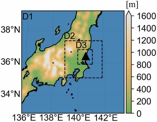
Table 1. Configuration of WRF for each domain.

Domain	D1	D2	D3
Horizontal grid points	78 × 78	88 × 88	103 × 103
Horizontal grid spacing (km)	9	3	1
Vertical layers	30
Time step (s)	36	12	4
Grid nudging	On	Off
Microphysics	Morrison microphysics [23]
Cumulus	Betts – Miller–Janjić Cumulus [24]		Off
Boundary layer	Mellor – Yamada–Nakanishi – Niino PBL Level 2.5 [25]
Surface layer	Mellor – Yamada–Nakanishi – Niino
Land surface	Five-layer thermal diffusion [21]
Shortwave radiation	Rapid radiative transfer model [26]
Longwave radiation	Dudhia [27]

Table 2. Configuration of GEARN for each domain.

Domain	D2	D3
Horizontal grid points	86 × 86	101 × 101
Horizontal grid spacing (km)	3	1
Vertical layers	28
Time step (s)	12	4
Output time interval (h)	1
Horizontal diffusion parameter	Pasquil – Gifford chart (stability: neutral)
Release point	NSRI (36.46°N, 140.60°E)
Release radionuclide	^137Cs
Release rate (Bq h^−1)	1
Release period (h)	1
Release height (m)	100
Particle number (h^−1)	10^6

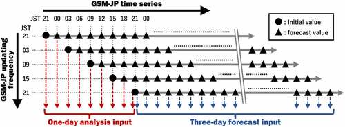
Input data from meteorological fields are required to drive WRF. The Grid Point Value of the Japan Meteorological Agency’s Global Spectral Model for the Japan area (GSM-JP) was used as the meteorological input. The GSM-JP datasets are distributed four times a day, which include analysis data at each initial time (0300, 0900, 1500, and 2100 JST; JST = UTC+9) created using a four-dimensional variational data assimilation method and forecast data for the next 84 h ahead with 3-h intervals. WRF calculations were conducted using two meteorological inputs: the analysis and forecast data. The meteorological input of the analysis data was constructed by accumulating the initial values in GSM-JP dataset at 2100, 0300, 0900, 1500, and 2100 JST (shown as filled circles in Figure 2) and 3-h forecast values at 0000, 0600, 1200, and 1800 JST (shown as filled triangles in Figure 2). However, for the meteorological input of the forecast data, each GSM-JP dataset was used exactly as is.

Figure 2. Illustration of the analysis and forecast inputs derived from the GSM-JP dataset.

Following the schematic as shown in Figure 2, the WSPEEDI-DB calculations for the 1-day analysis and 3-day forecast starting from 2100 JST using the meteorological analysis and forecast inputs, respectively, were conducted daily for 6 years from 31 December 2014. The ¹³⁷Cs tracer was released with the unit release conditions (1 Bq h⁻¹ for 1 h) from 100 m above the ground at the NSRI site four times per day (2100, 0300, 0900, and 1500 JST) during the calculation period. The plume distribution for each release was simulated from the release until after 6 h. The daily simulation results using the meteorological analysis and forecast inputs, in particular, contain a time series of four- and twelve-plume distributions with 6-h intervals up to 24 and 72 h, respectively. Therefore, by accumulating every day, 6 years of consecutive 6-hourly plume distributions (analysis outputs) were generated from simulation results with meteorological analysis inputs. On the other hand, simulation results with the meteorological forecast inputs for 3 days, each of which overlapped with the previous one for 2 days, were compiled to generate three plume distributions by different calculations every 6 h period for 6 years (forecast outputs).

2.3. Uncertainty estimation method

2.3.1. Index of plume direction: plume centroid

In this study, the plume centroid was introduced as an index of the plume direction, similar to the previous study [18]. The uncertainty of the forecasted plume direction was analyzed based on this index. The plume centroid is defined as a vector (G) from the release point to the center of the plume distribution, and the x- and y-components (G_x, G_y) are expressed as follows:

(1) $G_x=\frac{{\sum }_{i=1}^n{X}_{i}log\left(\frac{C_i}{C_0}\right)}{{\sum }_{i=1}^{n}log\left(\frac{C_i}{C_0}\right)},$(1)

(2) $G_y=\frac{{\sum }_{i=1}^n{Y}_{i}log\left(\frac{C_i}{C_0}\right)}{{\sum }_{i=1}^{n}log\left(\frac{C_i}{C_0}\right)},$(2)

where X_i and Y_i are the eastward and northward distances from the release point to the i-th grid point, respectively; C_i is the six-hourly averaged air concentration of ¹³⁷Cs in the bottom layer at the i-th grid point; n is the number of grid points in D3 (Figure 1); C₀ is the lower limit of the air concentration in the analysis. The weight using the logarithm was used to calculate the plume centroid, considering the low concentration in the downwind area and the high concentration near the release point. Additionally, the air concentration was normalized using C₀ to prevent the logarithm from reversing the relative magnitude of the air concentration. Because air concentrations less than 1.0 × 10⁻¹⁵ (Bq m⁻³) are equivalents to a statistical error in GEARN, the value of C₀ was set as 1.0 × 10⁻¹⁵ (Bq m⁻³). Also, because the half-life of ¹³⁷Cs is much longer than the simulation period of this study, the radioactive decay of ¹³⁷Cs in analyzing was ignored.

2.3.2. Bayesian machine learning

Generally, an analysis output is closer to the true value and thus, more reliable than the forecast output. Therefore, the uncertainty in the forecasted plume direction was evaluated by comparing the plume centroids in the forecast and analysis outputs in a previous study [18]. However, the study was unable to refer to the analysis output to estimate the uncertainty in the forecast output at the time of the forecast calculation. Therefore, a method was developed to predict the plume centroid in the analysis output from existing data at that time using Bayesian machine learning. A linear regression model was assumed to predict each component of the plume centroid in the analysis output as follows:

(3) $y_m=w^T{x}_m+{\text{isin}}_m,$(3)

where m indicates the index of data to determine the linear regression model, y_m is the predicted value of the m-th data, w is a weight vector and superscript T means transpose, and x_m and ${\text{isin}}_m$ are the vector of explanatory variables and error term for mth data, respectively. The optimum w and probability distribution of ${\text{isin}}_m$ were determined through the Bayesian machine learning using each component of the plume centroid in the analysis output (G^a) as a response variable and each component of the plume centroid in the forecast output as explanatory variables.

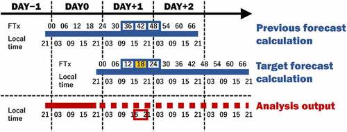
The previous study [18] reported that the discrepancy of plume direction between the forecast and analysis outputs increased because the small prediction differences in meteorological fields were temporally accumulated as the forecast time progression. The discrepancy of plume direction occasionally became 4–5 times higher than the annual average caused by the temporal or spatial gaps between forecast and analysis outputs in the passage of large meteorological variation. A linear regression model, which approximates locations of plume centroid, was determined for each 6-hourly forecast period to account for the trend in forecast time progression in the Bayesian machine learning (hereafter named FT00, FT06, FT12, etc., using the start time of the period in the forecast time, as shown in Figure 3). The plume centroids in the forecast outputs (G^f) at the three periods around the evaluation time were selected as explanatory variables to capture the passage of large meteorological variation. In addition to three periods, three corresponding periods were used from the forecast outputs calculated on the previous day. This was due to our expectation that the trend of plume direction change could be derived from the forecast outputs for the previous day using a daily update of calculations. For example, in the case of evaluating the uncertainty at the forecast period of FT18 (yellow shade in Figure 3), the corresponding plume centroid in the analysis output (a red box in Figure 3, 15 − 21 of local time in DAY+1) is predicted from FT12, FT18, and FT24 of the target forecast calculation and FT36, FT42, and FT48 of the previous forecast calculation (blue boxes in Figure 3). Therefore, for each evaluation time, six plume centroids in the forecast outputs (three periods × two forecast calculations) were used as the explanatory variables to model each component. Based on this setting, the predictable forecast periods were limited to those from FT06 to FT36 for which the six outputs were available.

Figure 3. Configuration of the analysis and forecast outputs used in the Bayesian machine learning. FTx indicates the 6-hourly forecast periods. The data in the analysis output, which is unavailable at the time of forecast calculation in DAY0, is shown as a red dashed-line.

The training and test data for the machine learning were randomly sampled from the forecast outputs. In this study, 80% of the total available data were used as training data, and the remaining data were used as test data. From the above procedure, the weight vector w for each forecast period was determined, and the model was validated using the test data. The probability distribution of the error term ${\text{isin}}_n$ was assumed to follow a normal distribution. Since the value of the variance of the normal distribution is repeatedly updated via Bayesian machine learning, the prior value of the variance σ² is required. In this study, the prior value at each forecast period was set to be equal to the variance of the input response variable at each period.

2.3.3. Uncertainty of plume directions

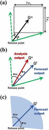
Figure 4 shows a schematic diagram regarding the method for evaluating the uncertainty of the plume direction. From the Bayesian machine learning, x- and y-components $\left(G_x^m,G_y^m\right)$ of the plume centroid G^m were modeled using the linear regression (3) and the probability distribution of the error term ${\text{isin}}_n$. The modeled plume centroid G^m was probabilistically distributed in the area determined using the normal distribution, where the G^m is the most probable and a rectangle area is defined with the widths of 2σ_x and 2σ_y for x- and y-directions, respectively, as shown in Figure 4(a). 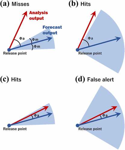The values of σ_x and σ_y are calculated along with a weight vector w when solving Equation (3)(3) $y_m=w^T{x}_m+{\text{isin}}_m,$(3) . From this distribution, a vector from the release point to a point included in the rectangle area was determined, which forms the maximum angle Φ (0° ≤ Φ < 180°) with G^m. Generally, the vector forming the maximum angle coincides with that pointing to one of the four corners of the rectangle area (solid green vector in Figure 4(a)). Then, a vector which forms line symmetry with this vector with respect to G^m was introduced (dashed green vector in Figure 4(a)). Finally, the uncertainty of the plume direction was defined as the angle Φ_m (0° ≤ Φ_m<180°). This angle was calculated from one of the two vectors forming the maximum angle Φ with G^m (dashed and solid green vectors in Figure 4(b)) and the vector of the plume centroid G^f in the forecast output (a blue vector in Figure 4(b)). In this study, of the two vectors (dashed and solid green vectors in Figure 4(b)), the one with the larger angle to G^f was adopted. Note that the angle is not distinguished between clockwise and counterclockwise. In case of Figure 4(b), the angle between the dashed green vector and G^f is adopted as the predicted uncertainty. From the above procedure, the uncertainty of the plume direction is shown as angles of Φ_m clockwise and counterclockwise to the forecasted plume direction, which is shown as a central angle with a light blue fan-shape in Figure 4(c). Similarly, the angle Φ_a formed by G^f and the vector of the plume centroid G^a in the analysis output was calculated (0° ≤ Φ_a<180°). Φ_a was used to investigate the validity of the predicted uncertainty of the plume direction Φ_m.

Figure 4. Schematic regarding the method for evaluating the uncertainty of the plume direction. G^m shown as a vector (black) with the release point as the origin and the rectangle area in (a) indicate the most probable point and probability distribution of the plume centroid calculated using the Bayesian machine learning, respectively. The solid and dashed green vectors in (a) and (b) are the one forming the maximum angle Φ with G^m and its line symmetrical one with respect to G^m, respectively. G^f and G^a in (b) indicate the vectors (blue and red, respectively) of the plume centroid from the forecast and analysis outputs, respectively. The predicted uncertainty of the plume direction is defined as the angle Φ_m to G^f, which is shown as a central angle with a light blue fan-shape in (c).

3. Results and discussion

3.1. Validation of the Bayesian machine learning

In this study, x- and y-components of the plume centroid G^m were modeled by applying the training data to the Bayesian machine learning. Multicollinearity, which causes computational instability in machine learning, is exhibited when the correlation between explanatory variables in the training data is strong. Therefore, the variance inflation factor (VIF) was used to investigate the possibility of multicollinearity. This statistic is an indicator of the severity of multicollinearity and is calculated as follows:

(4) $VIF={\left(1-R_e^2\right)}^{-1},$(4)

where $R_e^2$ is the coefficient of determination when regression is performed using an explanatory variable for which VIF is to be obtained as a response variable and other explanatory variables as explanatory variables. From the explanatory variables used in this study, the ranges of VIF for x- and y-components were calculated as 3.37–7.56 and 3.47–7.70, respectively. Generally, if the VIF statistic is 10 or higher, multicollinearity may be present [28]. Therefore, it is considered that the explanatory variables used in this study were adequately given to the Bayesian machine learning, and multicollinearity did not occur. Next, the coefficient of determination R² from the model using the training and test data was calculated (Table 3). The values of R² from the training and test data were the same level for each 6-hourly forecast period, indicating that the model is not overfitted. Therefore, it is thought that the model of the plume centroid using the Bayesian machine learning is reasonable.

Table 3. Coefficients of determination R² for the x- and y-components of the plume centroid estimated using Bayesian machine learning. The coefficients calculated from the training and test data are shown in the table.

6-hourly forecast period	Coefficients of determination R^2
	Gx		Gy
	Training	Test	Training	Test
FT06	0.991	0.990	0.989	0.990
FT12	0.959	0.953	0.953	0.956
FT18	0.917	0.907	0.927	0.920
FT24	0.853	0.851	0.868	0.859
FT30	0.802	0.811	0.805	0.766
FT36	0.828	0.782	0.805	0.791

3.2. Evaluation of predicted uncertainty

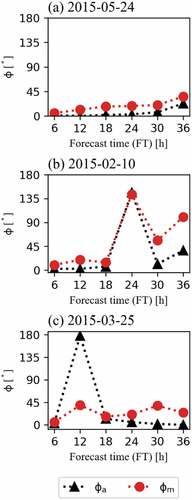
Before discussing the validity of the predicted uncertainty, the feature of Φ_a in this study was compared with that in the previous study [18]. Figure 5 shows the boxplot of Φ_a for each FT and Φ_m. The horizontal bars in the boxes and the open dots show the median and mean values, respectively. Overall, the angles of Φ_a, which were analyzed on the basis of the simulation results from 2015 to 2020, tended to increase with time (e.g. the mean value of Φ_a for FT24 was 16.8°). Although the analysis period of this study is different from that of Yoshida et al. [18], such temporal development feature of Φ_a agrees well with that of the previous study [18]. In addition, the angles of Φ_m showed the same feature except for the slightly larger temporal development. The previous study has reported that the angles of Φ_a can occasionally increase [18]. Such large angles of Φ_a are mostly plotted as outliers in figure. Figure 6 shows the typical time series of Φ_a and Φ_m obtained from our analysis. As shown in Figure 6, the angles of Φ_m well captured not only the monotonous time development of Φ_a (Figure 6(a)) but also the occasional angular increase in Φ_a in some cases (Figure 6(b)). However, it is unclear whether all outliers of Φ_m shown in Figure 5 adequately captures the angular increases in Φ_a such as the case of Figure 6(b). Therefore, the consistency between Φ_a and Φ_m was statistically analyzed using the method shown below. Additionally, there were a few cases where the angle increase in Φ_a was not captured (Figure 6(c)). Such cases are discussed in Section 3.3.

Figure 5. Boxplot of Φ_a (analysis) and Φ_m (model) for each FT. The top and bottom of the boxes indicate upper and lower quartiles, respectively; the horizontal bar in the box and an open circle show median and mean values, respectively; the upper and lower whiskers show the maximum and minimum angles. Respectively, except for outliers described outside the upper whisker.

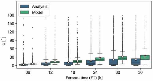
Figure 6. Time series of Φ_a (analysis) and Φ_m (model) from FT6 to FT36 on (a) May 24, (b) February 10, and (c) March 25, 2015. Black triangles and red circles indicate the angles from the analysis output and the Bayesian model, respectively.

To assess the validity of the predicted uncertainty Φ_m using Bayesian machine learning, we categorized its predictability of Φ_a as ‘hits,’ ‘misses,’ and ‘false alert’ from a conservative viewpoint of detecting the higher uncertainty of plume direction. Figure 7 shows the rates (%) for the judgement of ‘hits,’ ‘misses,’ and ‘false alert’ as a heatmap. In this study, the reproducibility for the ranges of angles Φ_a from 0° to 30° (low uncertainty), 30° to 60° (middle uncertainty), and 60° to 180° (high uncertainty) were evaluated. From these ranges and the predicted uncertainty Φ_m, the judgement for ‘hits,’ ‘misses,’ and ‘false alert’ was determined. The schematic regarding the judgment of ‘hits,’ ‘misses,’ and ‘false alert’ is shown in Figure 8. If the angles meet the condition of 30° ≤ Φ_a<180° and 0° ≤ Φ_m<30° or 60° ≤ Φ_a<180° and 30° ≤ Φ_m<60°, it is judged as ‘misses’ (Figure 8(a)). The rate for ‘misses’ is shown in three grids above the diagonal girds in Figure 7. In this case, the difference in plume direction between the analysis and forecast outputs is underestimated by the Bayesian model, showing the uncertainty of plume direction is not well predicted. Next, if the angles meet the condition of 30° ≤ Φ_a<60° and 30° ≤ Φ_m<60° or 60° ≤ Φ_a<180° and 60° ≤ Φ_m<180°, it is judged that the uncertainty estimation using the Bayesian model is ‘hits’ (Figure 8(b)). Similarly, when the angles meet the condition of 0° ≤ Φ_a<30° and 0° ≤ Φ_m<30°, this case is also judged as ‘hits’ (Figure 8(c)). Therefore, the diagonal grid in Figure 7 indicates ‘hits.’ These cases of comparable magnitudes of Φ_a and Φ_m show that the difference of plume direction between the analysis and forecast outputs is reasonably captured by the Bayesian model. Finally, if the angles meet the condition of 0° ≤ Φ_a<30° and 30° ≤ Φ_m<180° or 30° ≤ Φ_a<60° and 60° ≤ Φ_m<180°, it is judged as ‘false alert’ (Figure 7(d)). The rate for ‘false alert’ is shown in three grids below the diagonal girds in Figure 7. This case shows that the difference in plume direction between the analysis and forecast outputs is overestimated by the Bayesian model.

Figure 7. Heatmap showing the percentage of data contained in each domain. The horizontal and vertical axes show the values of Φ_a (analysis) and Φ_m (model), respectively. The value plotted in each domain indicates the percentage.

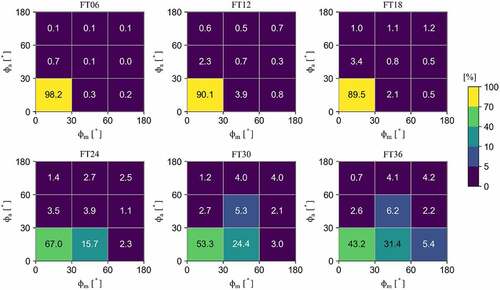
Figure 8. Schematic regarding the judgment of (a) ‘misses,’ (b) ‘hits’ for high uncertainty, (c) ‘hits’ for low uncertainty, and ‘false alert.’ the fan-shape colored as light blue indicates the uncertainty of forecasted plume direction.

Using the above conditions, rates of ‘hits,’ ‘misses,’ and ‘false alert’ were calculated for each 6-hourly forecast period. For FT06, most values of Φ_a and Φ_m were less than 30°. The ‘hits’ rate was 98.4% (= 98.2 + 0.1 + 0.1), showing that the Bayesian model accurately capture the difference in the plume directions between the analysis and forecast outputs. Additionally, the rates of ‘misses’ and ‘false alert’ were about 1%. For FT12 and FT18, the rates of ‘hits’ were 91.5% (= 90.1 + 0.7 + 0.7) and 91.5% (= 89.5 + 0.8 + 1.2), respectively. The rates of ‘misses’ and ‘false alert’ ranged from 3.4%−5.5% and 3.1%−5.0%, respectively, which was low as well as those for FT06. For FT24, the rate of ‘hits’ was 73.4% (= 67.0 + 3.9 + 2.5) and became somewhat lower than those for FT06, FT12, and FT18. Additionally, while the rate of ‘misses’ was still a low value of 7.6% (= 3.5 + 1.4 + 2.7), that of ‘false alert’ increased to 19.1% (= 15.7 + 1.1 + 2.3). For FT30 and FT36, the rates of ‘hits’ were 62.6% (= 53.3 + 5.3 + 4.0) and 53.6% (= 43.2 + 6.2 + 4.2), respectively. The rates of ‘misses’ were 7.4%−7.9%, which is as low as those for the other FTs. However, the rates of ‘false alert’ were further increased to 29.5% (= 24.4 + 2.1 + 3.0) and 39.0% (= 31.4 + 2.2 + 5.4), compared to those for FT24.

Throughout all cases from FT06 to FT36, the Bayesian model-based uncertainty assessment reasonably captured the differences in the plume direction between the analysis and forecast outputs. Even in the predictions made after 36 h, the differences could be quantitatively evaluated at a rate of about 50%. Here, the value of Φ_m from 0° to 30° was the focus. At this angle, the difference in the plume direction between the forecast output and the Bayesian model was comparably small. This implies that the uncertainty of the forecast output contained in the angle is small, and the prediction by WSPEEDI-DB is reliable. Under the reliable prediction case (0° ≤ Φ_m<30°), the rate of ‘hits’ for FT06 was calculated as 99.2% (= 98.2/(98.2 + 0.7 + 0.1) × 100). Similarly, the rates from FT12 to FT36 were calculated as 92.9%−96.9%. These high percentages show that when the difference in the plume direction between the Bayesian model and the forecast output is small, particularly 0° ≤ Φ_m<30°, the plume direction in the forecast output well represents the plume direction in the analysis output.

3.3. Predictability of “misses”

When predicting the atmospheric dispersion of radionuclide plumes during a nuclear accident, from the standpoint of safety, it is important to increase ‘hits’ and reduce ‘misses.’ From Figure 8, the rates of ‘misses’ from FT06 to FT36 were 0.9%−7.9%, and it was discovered that the rates of ‘misses’ were low throughout the forecast time. However, it is necessary to grasp the possibility of ‘misses’ in advance because the decision (for example, an evacuation order) based on a result including ‘misses’ could lead to serious events, such as health hazards to the public. A judgment of ‘misses,’ where the actual plume can deviate significantly from the forecast, is very threatening, especially when the uncertainty is evaluated as small (0° ≤ Φ_m<30°). As mentioned above, the angles Φ_a and Φ_m occasionally increased (Figure 5). In this study, judgments of ‘misses’ mostly occurred when the angles became temporally large.

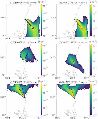
Figure 9 shows the horizontal distribution of ¹³⁷Cs concentration from FT06 to FT18 on 25 March 2015. Figure 6(c) shows the time series of Φ_a and Φ_m on this day. This temporal development of the ¹³⁷Cs concentration describes a typical case of ‘misses’ in the simulation. For FT06, the plumes were distributed in the southeast area of the release point (Figures 9(a,b)). The plume distribution was well reproduced in the forecast output more than in the analysis output (Φ_a = 3.3°), and the locations of the plume centroid in both outputs were close to each other (Figures 9(a,b)). Further, the location of the plume centroid obtained from the Bayesian machine learning was well predicted for the analysis output (Φ_m = 5.5°, low uncertainty). For FT12, the plumes were transported northward across the release point and were distributed over the release point because the southerly wind was enhanced (wind is not shown in the figures). During the northward transportation, the plume centroids in the forecast and analysis outputs were located on the north and south sides of the release point, respectively (Φ_a = 177.8°) (Figures 9(c,d)). Also, the plume centroid obtained from the Bayesian machine learning was located on the north side of the release point (Φ_m = 39.3°, middle uncertainty), which was significantly different from that in the analysis output. For FT18, the plume in the forecast output showed a distribution similar to that in the analysis output, and the location of the plume centroid in the forecast output was in the neighbor of that by the analysis output (Φ_a = 12.2°) (Figures 9(e,f)). Similarly, the plume centroid obtained from the Bayesian machine learning was located near the plume centroid in the analysis output (Φ_m = 16.5°, low uncertainty).

Figure 9. Horizontal distribution of ¹³⁷Cs concentration from FT06 to FT18 on March 25, 2015. The triangle symbol shows the location of the release point. The left and right columns of the figure show the results of the forecast and analysis outputs, respectively. Black and blue lines in the left column describe the vector indicating the plume centroid (shown as a filled circle at the line end) by the forecast output and the Bayesian model, respectively. The dashed red line in the left column and the red line in the right column describe the vector indicating the plume centroid by the analysis output.

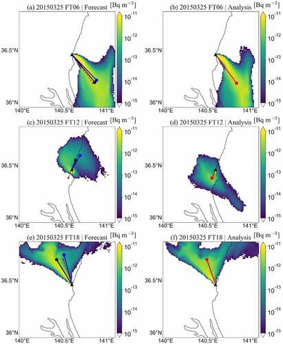
In the case on March 25, there was no precipitation (not shown in Figure 9) in the simulation domain. This implies that there was no contribution of the wet deposition to the plume distribution. However, as mentioned above, the wind direction changed from northernly to southernly for the time of FT12. The change in the wind direction that appeared in the forecast output was also seen in the analysis output. For these reasons, it is thought that the plume distribution from the forecast output showed a different pattern from the analysis output. This is because of the slight difference in the variation of the wind direction between the forecast and analysis output. When comparing the plume centroid, the plume centroid from the forecast output was located on the other side across the release point to that from the analysis output. Although the plume centroids were geographically close to each other, the case on March 25 was judged as ‘misses.’ Again, the changes in wind direction were predicted in the forecast output. Therefore, when large changes in wind direction occur in the forecast output, as in the case of March 25, it may be possible in advance to warn of the occurrence of ‘misses’ based on the large changes of wind direction. However, it is difficult to determine the occurrence of ‘misses’ with certainty. This would be considered the limitation of the uncertainty estimation method using the angle calculated with plume centroid.

4. Conclusion

This study developed an uncertainty estimation method for atmospheric dispersion simulations using WSPEEDI-DB developed by the JAEA. The difference in plume directions derived from the meteorological forecast and analysis inputs was the focus for estimating the uncertainty, since the plume direction would be the most important information in the emergency responses to avoid the exposure to the radioactive plume. The uncertainty of the plume direction was defined as a variation range of the discrepancy angle from the forecasted plume direction, which was simple and easy to grasp the variability of plume direction. A vector was introduced to represent the location of the plume centroid as the plume direction. The vector was modeled using Bayesian machine learning, with the analysis output (response variables) and the forecast output (explanatory variables) provided by the WSPEEDI-DB database. Then the vector modeled using the Bayesian machine learning was compared with those from the analysis and forecast outputs to confirm the validity of the Bayesian model of this study.

It was first confirmed that the Bayesian model of the vectors was not overfitted, with the same-level values of the coefficient of determination R² between the training and test data. Additionally, it was shown that the explanatory variables were reasonably used in this study from the VIF index analysis. In the uncertainty evaluation, it was discovered that the rate of ‘hits’ (good prediction of uncertainty) was at least 50%, although it decreased with forecast time. However, ‘false alert’ (over-prediction of higher uncertainty) was often observed, with a rate up to 31.2% for FT = 36 h. Additionally, it was discovered that the rate of ‘misses’ (under-prediction of higher uncertainty) was low with a range of 0.9%−7.9%. These results indicate that the proposed method for uncertainty estimation can be reasonably used from a safety standpoint. The judgments of ‘misses’ mainly resulted from the different distribution of the plume due to significant wind direction changes. Particularly, when the plume centroid is located in the vicinity of the release point, a slight difference in the distribution affects the judgment. In this study, a Bayesian statistics model was developed using the angles formed by the line segments connecting the two plume centroids from the forecast output, analysis output, and release point. In addition to the angles, a more reliable model may be developed if the distance between the plume centroid and the release point is further employed as explanatory variables for the Bayesian machine learning. Also, deep learning modeling may enable quantifying the uncertainty of the plume distribution from the forecast output with more accuracy. When developing the statistics model, we assumed a linear regression model. However, there is no clear metric that determines the shape of the model, and using different model shapes, such as logarithmic or exponential may alter the results. Deep learning modeling would improve such uncertainties in Bayesian machine learning attributed to the shape of the statistics model. In addition, the ATDM using a large-eddy simulation with a finer spatial resolution than that in this study has been developed [29,30]. It is also planned to investigate the applicability of the uncertainty estimation method proposed in this study to the finer resolution and local scale. The predicted uncertainty of the plume direction is shown by appending two fan-shapes with the angle of Φ_m, which shows the variation range of discrepancy angle, on both side of the forecasted plume direction. In the future, we need to further consider how to express the uncertainty from this study, taking into account the ease of understanding for users.

When conducting ATDM simulations, the uncertainty of simulation results is often quantified from ensemble means using multiple models or ensemble simulations using a single model [6–13]. The proposed method can address the uncertainty of the simulation results without using many models or conducting ensemble simulations based on various scenarios. In a nuclear emergency, a quick response is required to understand the contamination state attributed to radionuclides by developing evacuation plans for the public. The method proposed in this study enabled an estimation of the uncertainty of atmospheric dispersion simulations from only forecast outputs without referring to analysis outputs. From a combination of Bayesian machine learning and the database of atmospheric dispersion of radionuclides calculated in advance using WSPEEDI-DB, the information in terms of radionuclide distribution in the environment would be quickly provided under the emergency, with their uncertainty. When assisting the emergency responses during a nuclear emergency, such information would be useful with available monitoring data.

Disclosure statement

No potential conflict of interest was reported by the authors.

Supplementary material

Supplemental data for this article can be accessed online at https://doi.org/10.1080/00223131.2023.2177763.

References

- Imai K, Chino M, Ishikawa H. SPEEDI: A computer code system for the real-time prediction of radiation dose to the public due to an accidental release. JAERI–1297. Japan: Japan Atomic Energy Research Institute; 1985. p. 93.
- Nagai H, Chino M, Yamazawa H. Development of scheme for predicting atmospheric dispersion of radionuclides during nuclear emergency by using atmospheric dynamic model. J At Energy Soc Jpn. 1999;41(7):777–785. in Japanese.
- Headquarters NER report of Japanese government to the IAEA ministerial conference on nuclear safety – The accident at TEPCO’s Fukushima Nuclear Power Stations. Tokyo: Government of Japan; 2011. [cited 2022 Oct 25] Available from: https://japan.kantei.go.jp/kan/topics/201106/iaea_houkokusho_e.html
- Galmarini S, Bianconi R, Klug W, et al. Ensemble dispersion forecasting—Part I: concept, approach and indicators. Atmos Environ. 2004;38(28):4607–4617. DOI:10.1016/j.atmosenv.2004.05.030
- Galmarini S, Bianconi R, Addis R, et al. Ensemble dispersion forecasting—part II: Application and evaluation. Atmos Environ. 2004;38(28):4619–4632. DOI:10.1016/j.atmosenv.2004.05.031
- Draxler R, Arnold D, Chino M, et al. World Meteorological Organization’s model simulations of the radionuclide dispersion and deposition from the Fukushima Daiichi nuclear power plant accident. J Environ Radioact. 2015;139:172–184.
- Kitayama K, Morino Y, Takigawa M, et al. Atmospheric modeling of 137Cs plumes from the Fukushima Daiichi nuclear power plant—Evaluation of the model intercomparison data of the science council of Japan. J Geophys Res Atmos. 2018;123:7754–7770.
- Sato Y, Takigawa M, Sekiyama TT, et al. Model intercomparison of atmospheric 137Cs from the FUkushima Daiichi nuclear power plant accident: simulations based on identical input data. J Geophys Res Atmos. 2018;123(20):11–748. DOI:10.1029/2018JD029144
- Sato Y, Sekiyama TT, Fang S, et al. A model inter- comparison of atmospheric 137Cs concentrations from the Fukushima Daiichi nuclear power plant accident, phase III: simulation with an identical source term and meteorological field at 1-km resolution. Atmos Environ X. 2020;7(100):086. DOI:10.1016/j.aeaoa.2020.100086
- Kajino M, Sekiyama TT, Igarashi Y, et al. Deposition and dispersion of radio-cesium released due to the Fukushima nuclear accident: sensitivity to meteorological models and physical modules. J Geophys Res Atmos. 2019;124(3):1823–1845. DOI:10.1029/2018JD028998
- Kajino M, Sekiyama TT, Mathieu A, et al. Lessons learned from atmospheric modeling studies after the Fukushima nuclear accident: ensemble simulations, data assimilation, elemental process modeling, and inverse modeling. Geochem J. 2018;52(2):85–101. DOI:10.2343/geochemj.2.0503
- Iwasaki T, Sekiyama TT, Nakajima T, et al. Intercomparison of numerical atmospheric dispersion prediction models for emergency response to emissions of radionuclides with limited source information in the Fukushima Dai-ichi nuclear power plant accident. Atmos Environ. 2019;214:116,830.
- Korsakissok I, Périllat R, Andronopoulos S, et al. Uncertainty propagation in atmospheric dispersion models for radiological emergencies in the pre- and early release phase: summary of case studies. Radioprot. 2020;55:S57–68.
- Yoshida T, Nagai H, Terada H, et al. Evaluation of uncertainties derived from meteorological forecast inputs in plume directions predicted by atmospheric dispersion simulations. J Nucl Sci Technol. 2022;59(1):55–66. DOI:10.1080/00223131.2021.1951862
- Terada H, Nagai H, Tanaka A, et al. Atmospheric-dispersion database system that can immediately provide calculation results for various source term and meteorological conditions. J Nucl Sci Technol. 2020;57(6):745–754. DOI:10.1080/00223131.2019.1709994
- Kim JY, Lee SH, Park TJ. A Methodology for Estimating the Uncertainty in Model Parameters Applying the Robust Bayesian Inferences. J. Radiat Prot Res. 2016;41(2):149–154.
- Smith J, French S. Bayesian Updating of Atmospheric Dispersion Models for Use After an Accidental Release of Radioactivity. J R Stat Soc. 1993;42(5):501–511.
- Terada H, Nagai H, Tsuduki K, et al. Refinement of source term and atmospheric dispersion simulations of radionuclides during the Fukushima Daiichi Nuclear Power Station accident. J Environ Radioact. 2020;213:106104.
- Kim JY, Jan HK, Lee JK. The Robust Bayesian Analysis Due to a Variation of Effective Height in the Atmospheric Dispersion. J Nucl Sci Technol. 2008;45(5):710–713.
- Gunawardena N, Pollotta G, Simpson M, et al. Machine Learning Emulation of Spatial Deposition from a Multi-physics Ensemble of Weather and Atmospheric Transport Models. Atmosphere. 2021;12(8):953. DOI:10.3390/atmos12080953
- Skamarock WC, Klemp JB, Dudhia J, et al. A description of the advanced research WRF version 3. USA: National Center for Atmospheric Research; 2008. (NCAR/TN-475STR).
- Terada H, Chino M. Development of an atmospheric dispersion model for accidental discharge of radio nuclides with the function of simultaneous prediction for multiple domains and its evaluation by application to the Chernobyl nuclear accident. J Nucl Sci Technol. 2008;45(9):920–931.
- Morrison H, Thompson G, Tatarskii V. Impact of cloud microphysics on the development of trailing stratiform precipitation in a simulated squall line: Comparison of one-and two-moment schemes. Mon Wea Rev. 2009;137(3):991–1007.
- Janjić ZI. The step-mountain eta coordinate model: Further developments of the convection, viscous sublayer, and turbulence closure schemes. Mon Wea Rev. 1994;122(5):927–945.
- Nakanishi M, Niino H. An improved Mellor–Yamada level-3 model with condensation physics: Its design and verification. Bound-Lay Meteorol. 2004;112(1):1–31.
- Mlawer EJ, Taubman SJ, Brown PD, et al. Radiative transfer for inhomogeneous atmospheres: RRTM, a validated correlated-k model for the longwave. J Geophys Res Atmos. 1997;102(D14):16663–16682. DOI:10.1029/97JD00237
- Dudhia J. Numerical study of convection observed during the winter monsoon experiment using a mesoscale two-dimensional model. J Atmos Sci. 1989;46(20):3077–3107.
- Montgomery DC, Peck EA. Introduction to Linear Regression Analysis. New York: Wiley; 1992.
- Nakayama H, Satoh D, Nagai H, et al. Development of local-scale high-resolution atmospheric dispersion model using large-eddy simulation part 6: introduction of detailed dose calculation method. J Nucl Sci Technol. 2021;58(9):949–969. DOI:10.1080/00223131.2021.1894256
- Nakayama H, Onodera N, Satoh D, et al. Development of local-scale high-resolution atmospheric dispersion and dose assessment system. J Nucl Sci Technol. 2022;59(10):1314–1329. DOI:10.1080/00223131.2022.2038302