The effect of using Filtered Containment Venting System on variation in dose with distance in the prompt accident consequence assessment

ABSTRACT

In a nuclear emergency, consequence assessment based on the plant conditions using a simple method is important for a prompt response. Response Technical Manual (RTM-96) is a manual calculation method for prompt dose projection at arbitrary distances by converting pre-calculated doses with the conversion factor based on distance and weather. However, the ‘conversion factor’ in RTM-96 does not consider accident scenarios with filtered containment venting system (FCVS). Therefore, in this study, we defined the ratio of effective dose between 1 km and an arbitrary distance as the ‘Distance Conversion Factor (DCF)’ and aimed to clarify the difference between DCFs by accident scenarios, focusing on the presence or absence of FCVS. The results showed that the differences in DCFs for different accident scenarios were minor in the case of no rainfall. In contrast, in the case of rainfall, DCF differed significantly with scenarios with FCVS and those with containment failure. Therefore, the authors propose that DCFs with rainfall should be calculated separately for several representative accident scenarios rather than uniformly for all accident scenarios, as in the conventional method. The results can contribute to developing a new prompt consequence assessment method, such as RTM-96, which considers FCVS.

KEYWORDS:

• RTM-96
• emergency response
• FCVS
• aerosol
• gas
• washout
• deposition
• variation in dose with distance
• Distance Conversion Factor (DCF)

1. Introduction

In the event of a severe accident at a nuclear power plant, a prompt accident consequence assessment based on the plant conditions (status of the reactor core and release pathway conditions) is necessary [1–3]. Recent studies have focused on understanding the magnitude of accidents based on radiological impact. For instance, research has been conducted where severe accident scenarios are selected to evaluate the distances exceeding established dose limits [4]. In another study, various assumed decontamination factors have been used to predict dose at different distances, and the study has assessed the radiological impact of nuclear accidents corresponding to these scenarios [5]. These research efforts primarily emphasize nuclear safety and emergency preparedness.

On the other hand, dose projection with each distance and assessing the magnitude of accidents based on the plant conditions not only pertains to the fields targeted in the beforementioned studies but also contributes to emergency response. A considerable number of studies have been reported where, after a period following an accident and once monitoring data becomes available, a more detailed source term (such as release timing, magnitude, and duration of fission product release) assessment and subsequent dose estimation are conducted based on the monitoring information [6,7]. However, particularly in the immediate aftermath of an accident, when information about the source term is limited, it is crucial to conduct prompt evaluations with the limited information available. In particular, dose projection in each distance based on plant conditions is essential to confirm or modify protective action recommendations, and a simple estimation of variation in dose with distance can contribute to a prompt decision. Although analysis codes such as RASCAL [8] and RASTES [9] exist for projecting doses during emergencies, a method to perform such assessments using only simple manual calculations quickly and easily on paper is important during an emergency.

The Response Technical Manual [2] (RTM-96) is a method for quickly estimating the dose as a function of distance using simple manual calculations. It is a well-known method for prompt consequence assessment in an emergency, and TECDOC-955 [10] by IAEA incorporates its methodology. In RTM-96, the pre-calculated dose at a 1-mile point is described based on the plant conditions, and the dose downwind is calculated using a Distance Conversion Factor (in this study, this conversion factor is called DCF) as a function of distance for different weather conditions. However, these conversion factors in RTM-96 were defined uniquely without considering differences in accident scenarios.

Many other studies which focused on variation in dose with distance have been conducted in the past. For example, the variation in bone marrow doses and effective doses with distance over 4 days was studied for several atmospheric stabilities and wind speeds in NUREG-1940 [8]. The U.S. PAG manual [3] provided simple formulas to evaluate dose over distance using manual calculations. The case where rainfall was considered was discussed in the RASCAL2.1 manual [11] and the RASCAL2.1 workbook [12]. Although these studies considered variation in dose with distance considering multiple meteorological conditions, they did not address the effects of different accident scenarios.

For dose projection in an emergency, it is essential to be able to perform calculations under specific meteorological conditions with or without rainfall. Therefore, this study aims to clarify the effect of different accident scenarios on the variation in dose downwind with distance from the release point.

The differences between the approach presented in this study and RTM-96 are as follows: First, this study expands the discussion on Filtered Containment Venting System (FCVS) [13,14], which are not addressed in RTM-96. Furthermore, the contribution of aerosols to dose in each accident scenario is focused on, and the impact of various levels of rainfall on variation in dose with distance was quantitatively evaluated, which is a new consideration not addressed in RTM-96. Finally, instead of just presenting values of DCF as in RTM-96, this study shows the formulas of DCF.

2. Material and method

2.1. Overview of RTM-96 calculations

RTM-96 introduces a way to pre-calculate doses based on the plant conditions to perform quick calculations in an emergency [2]. Figure 1 shows the schematic diagram of the RTM-96 calculation flow.

Figure 1. The schematic diagram of the simplified RTM-96 calculation flow.

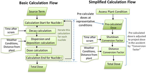
In the basic method of calculating doses, the source term (the timing, magnitude, and duration of fission product releases) is used as input, then decay, atmospheric transport, deposition, and doses for each nuclide are calculated, and the doses for all nuclides released are finally added up. On the other hand, in RTM-96, a pre-calculated dose based on the plant conditions is used and converted using conversion factors to project the dose in the accident [2]. This simple method of multiplying the conversion factor by pre-calculated doses for each plant condition has the advantage that RTM-96 [2] can perform calculations promptly in an emergency. According to RTM-96, this method can estimate the centerline dose on the downwind direction within an error factor of 10–100 if the plant, release height, and rain conditions are accurately represented.

Pre-calculated doses are written in event trees based on the status of the reactor core and release pathways in RTM-96 [2]. In this study, the combination of core conditions and release paths represented by each sequence in the event tree is called an ‘accident scenario.’ In the event tree, pre-calculated dose estimates are written to determine the offsite consequences of a reactor accident. The pre-calculated dose in each event tree is based on a dose to an individual, assuming average weather conditions (D stability, wind speed 1.8 m/s, no rain), a 1-h release duration, and no sheltering or protection at a point along the centerline of the plume. The Effective Dose includes the inhalation from the passing plume, the external dose from the passing plume (cloudshine), and the dose from exposure to the contaminated ground (groundshine). The core conditions and release conditions, which significantly affect the dose, are considered. The pre-calculated doses based on the plant conditions listed in the event tree are converted by conversion factors shown in Figure 1. The subject of this study is the Distance Conversion Factor (DCF), which is used to convert the pre-calculated doses based on the distance and the weather conditions. RTM-96 lists values for DCF for bone marrow dose and thyroid dose. However, RTM-96 does not describe how they are derived [2]. These conversion factors are needed to calculate the dose at 1 mile or for other distances and release conditions. DCF of RTM-96 is set as the representative value with or without rainfall, independent of the accident scenario.

In RTM-96, the bone marrow and thyroid dose were evaluated [2], while in this study, the effective dose was newly evaluated. Alongside thyroid or bone marrow dose, effective dose is a crucial assessment metric for assessing the radiological consequences and evaluating emergency responses. By incorporating the consideration of effective dose, rapid dose projection methods like RTM-96 can be utilized to compare the IAEA Generic Criteria, which stipulates a 100 mSv effective dose in the first 7 days as a criterion for urgent protective actions such as evacuation or sheltering [15]. In countries such as Japan, an effective dose of 100 mSv in the first 7 days is used as one of the references for setting standards for protective actions [16]. Thus, the DCF corresponding to effective dose is examined in this study.

Also, in this study, the authors present a novel enhancement to the RTM-96 model by incorporating FCVS. This unique safety feature was installed in Japanese nuclear power plants following the Fukushima Daiichi nuclear accident. This inclusion of FCVS is a significant advancement, enabling us to consider a broader range of accident scenarios than before. By modifying the event tree’s end nodes and introducing new accident scenarios considering FCVS, our approach not only allows us to capture a wider variety of potential nuclear accident situations but also reflects the lessons learned from the Fukushima Daiichi nuclear accident, making our model more relevant and adaptable to the plans complying with new regulatory standards.

2.2. Influence of accident scenario on variation in dose with distance

The following describes the calculation method used in this study to calculate the variation in dose with distance, which is expressed as the DCF in each accident scenario. In this study, DCF $F_p\left(\mathit{x}\right)$ in each accident scenario is defined by Equation 1(1) $F_p\left(\mathit{x}\right)=\frac{H_p\left(\mathit{x}\right)}{H_{\mathit{norain}}\left(1\right)}$(1) as follows.

(1) $F_p\left(\mathit{x}\right)=\frac{H_p\left(\mathit{x}\right)}{H_{\mathit{norain}}\left(1\right)}$(1)

where $F_p\left(\mathit{x}\right)$ is the DCF which converts the pre-calculated dose to the arbitrary downwind distance from the release point and weather (-), $H_p\left(\mathit{x}\right)$ is the effective dose $\left(\mathrm{Sv}\right)$ at downwind distance $\mathit{x}\left(\mathrm{km}\right)$ and weather condition $\mathit{p}$, and $H_{\mathit{norain}}\left(1\right)$ is the pre-calculated effective dose $\left(\mathrm{Sv}\right)$ at downwind distance $\mathit{x}$ is $1\left(\mathit{km}\right)$ and weather condition $\mathit{p}$ is $\mathit{norain}$.

The denominator is the pre-calculated dose at the reference of 1 km distance and weather in the event tree, and the numerator is the dose at any distance and weather.

Both $H_p\left(\mathit{x}\right)$ and $H_{\mathit{norain}}\left(1\right)$ were calculated in the same conditions except for distance and weather. In this study, DCF $F_p\left(\mathit{x}\right)$ was calculated for each accident scenario. Then, the differences in DCF for different accident scenarios with and without rainfall were compared to clarify the characteristics of the conversion factor based on the characteristics of the accident scenario. Finally, based on the calculated DCF for each scenario $F_p\left(\mathit{x}\right)$, the authors proposed a DCF that could accommodate multiple accident scenarios; since the DCF in RTM-96 is defined as representative of accident scenarios, this study similarly defined it in a manner that encompasses the multiple accident scenarios. This approach ensures rapid calculations in emergencies.

The effective dose $H_p\left(\mathit{x}\right)$ was calculated using three steps. The details are described in the subsequent sections.

1. Calculation of release of nuclides to the environment for each accident scenario　

2. Calculation of air and surface contamination concentrations　

3. Conversion of air and surface contamination concentrations to effective dose　

2.3. Atmospheric release for different accident scenarios

Calculating the amount and isotopic composition of material released followed the method is described in RTM-96 [2]. That is, radionuclides released to the environment were calculated as the product of the initial inventory, the rate of release of each radionuclide from the core to the containment (Core Release Fraction), the reduction factor in the containment (Reduction Factor), and the leakage rate from containment or primary coolant system to the environment (Escape Fraction). Radionuclides released to the environment are calculated as follows:

(2) $\dot{Q_i}=Q_i^{\mathit{INV}}\times F_i^{\mathit{CRF}}\times F_i^{\mathit{RDF}}\times F^{\mathit{EF}}\mathit{\hspace{0.17em}}$(2)

where $Q_i$ is the rate of radioactivity release to the environment for each nuclide $\mathit{i}$ (Bq/h), $Q_i^{\mathit{INV}}$ is the core inventory of radionuclide$\mathit{i}$ (Bq) [2,17], $F_i^{\mathit{CRF}}$ is the ratio of the amount of radionuclide $\mathit{i}$ released from the core to its initial core inventory (-) [2,18], $F_i^{\mathit{RDF}}$ is the ratio of the amount of radionuclide $\mathit{i}$ available for release after reduction mechanism to that available for release before this reduction mechanism, which corresponds to reciprocal of the Decontamination Factor (DF) (-) [2,19], and $F^{\mathit{EF}}$ is the leakage rate of the containment or primary coolant system (1/h) [2,19], respectively.

The accident scenarios considered for calculating DCF are shown in Table 1. In this study, accident scenarios that have a significant impact beyond 1 km were targeted since there are four types of core conditions in RTM-96: (1) normal, (2) spike, (3) gap release, and (4) in-vessel core melt. The (1) normal and (2) spike are the type of design basis accident, i.e. scenarios in which core damage has not occurred. Since the effective dose beyond 1 km is extremely small for these scenarios, only scenarios (3) and (4) were considered for calculating DCF. The assumed core conditions are expressed as $F_i^{\mathit{CRF}}.$ The values of $F_i^{\mathit{CRF}}$ were taken from NUREG-1465 [18].

Table 1. Accident scenarios considered in this study.

Release type	Scenario name	Accident scenarios
Bypass	g1	PWR steam generator tube rupture with a release of coolant contaminated due to a gap release from the core
	g2	PWR steam generator tube rupture with a release of coolant contaminated due to in-vessel core melt
	ν1	BWR/PWR containment bypass release for a gap release
	v2	BWR/PWR containment bypass release for an in-vessel core melt release
Containment Release without Scrubbing	δ1	PWR large dry or subatmospheric containment release for a gap release
	δ2	PWR large dry or subatmospheric containment release for an in-vessel core melt release
	δ3	BWR containment dry-well release for a gap release
	δ4	BWR containment dry-well release for an in-vessel core melt release
Containment Release with Scrubbing	δ5	BWR containment wet-well release for a gap release
	δ6	BWR containment wet-well release for an in-vessel core melt release
Release with FCVS	φ1	PWR large dry or subatmospheric containment release for a gap release with FCVS
	φ2	PWR large dry or subatmospheric containment release for an in-vessel core melt release with FCVS
	φ3	BWR containment dry-well release for a gap release with FCVS
	φ4	BWR containment dry-well release for an in-vessel core melt release with FCVS
	φ5	BWR containment wet-well release for a gap release with FCVS
	φ6	BWR containment wet-well release for an in-vessel core melt release with FCVS

Further, for each release category, when the mechanism for removing radionuclides is significant (i.e. when the filter effect or scrubbing effect is substantial), the $F_i^{\mathit{RDF}}$ becomes a smaller value, indicating a reduction in the release of radionuclides to the environment. Pathways and core conditions, i.e. various mitigation effects such as filter are considered as $F_i^{\mathit{RDF}}$. The effect of $F_i^{\mathit{RDF}}$does not apply to noble gases.

$F^{\mathit{EF}}$ expresses the release rate to the environment. The value is set for each containment condition (i.e. design leak, failure to isolate, design leakage, etc.).

A PWR Steam Generator Tube Rupture (SGTR) release assumes contaminated coolant leaks through the rupture. When the steam generator is partitioned, particulates are retained in the steam generator water and are not released.

A PWR/BWR containment bypass release assumes a release through the dry pathway from the primary system out of the containment. Filtering (not FCVS) through the release pathway can be considered in some scenarios of this category.

A PWR dry containment release and BWR dry-well containment release assume a release into the containment, which leaks into the atmosphere. The effectiveness of sprays or natural processes (plate-out) can be considered.

BWR wet-well containment release assumes a release through the suppression pool. This category is the closest to the scenarios with hardened containment venting system (HCVS) which relies solely on the scrubbing of BWR’s Wet-Well (W/W), without involving a filter. HCVS is used as ‘vent’ before introduction of FCVS and it attempted in the Fukushima Daiichi nuclear accident.

For the scenarios with FCVS, not considered in the past study [2], 0.001 for aerosol, 0.01 for elemental iodine, and 0.02 for organic iodine [13] were used as $F_i^{\mathit{RDF}}$. Thus, the environment release fraction of aerosol nuclides is small. The environmental release fractions to the initial core inventory of each of the nuclides are shown in the supplementary online material.

2.4. Calculation of air concentration and ground contamination

The calculation of air concentration (Bq/m³) was performed using the Gaussian Plume Model based on the method described in the Meteorological Guidelines [20]. This model is also used in the Atomic Energy Society of Japan (AESJ)‘s Level 3 Probabilistic Risk Assessment (PRA) standard [21] and is also used in the RTM-96 [2] calculations. The wind speed and atmospheric stability were 1.8 m/s and D [2], respectively, and diffusion parameters were calculated based on Meteorological Guidelines [20] and considered building wake correction [22]. This method is like the approach used in RTM-96 to calculate diffusion. The air concentrations by nuclide are as follows:

(3) ${\chi }_i\left(\mathit{x},\mathit{y},\mathit{z}\right)=\dot{Q_i}\times \mathit{\chi }/\mathrm{Q}\times \mathit{\hspace{0.17em}}exp\left(-{\lambda }_i\mathit{t}\right)\times \mathit{exp}\left(-\mathrm{\Lambda }\frac{x}{u}\right)\times f_F$(3)

where $Q_i$ is radioactivity released to the environment for each nuclide calculated in Section 2.3 (Bq/s),¹$\mathit{\chi }/\mathrm{Q}$ is relative air concentration (s/m³) [20], ${\lambda }_i$ is the decay constant (s⁻¹), t is time to reach the residential point from scram (s), which is defined as $\mathit{t}=t_{\mathit{rel}}$+$\frac{x}{u}$, $t_{\mathit{rel}}$ is the time from scram to release (s),$\frac{x}{u}$ is the time from release to the residential point,$\mathrm{\Lambda }$ is the washout coefficient² (s⁻¹) [23], $\mathit{x}$ is downwind distance (m), $\mathit{u}$ is wind speed (m/s), and $f_F$ is source depletion coefficient by dry deposition (-) [21,24], respectively.

The relative air concentration $\mathit{\chi }/\mathrm{Q}$ is defined using Gaussian Plume Model as follows:

(4) $\mathit{\chi }/\mathrm{Q}=\frac{1}{2\pi {\sigma }_y{\sigma }_z\mathit{u}}\mathit{exp}\left(-\frac{y^2}{2{\sigma }_y^2}\right)\left[\mathit{exp}\left\{-\frac{{\left(\mathit{z}-\mathit{h}\right)}^2}{2{\sigma }_z^2}\right\}\text{break}+\mathit{exp}\left\{-\frac{{\left(\mathit{z}+\mathit{h}\right)}^2}{2{\sigma }_z^2}\right\}\right]$(4)

where $\mathit{y}$ is the horizontal distance (m), $\mathit{z}$ is vertical distance (m), ${\sigma }_y$ is horizontal dispersion coefficient (m) [20,22], ${\sigma }_z$ is vertical dispersion coefficient (m) [20,22], $\mathit{h}$ is the release height (m), respectively. In this paper, ground-level release is focused on.

In this study, the centerline dose on the ground was evaluated, so $\mathit{y}$, $\mathit{z}$ was set to zero.

The depletion factor due to dry deposition is calculated as follows.

(5) $f_F=\mathit{exp}\{-\sqrt{\frac{2}{\pi }}\frac{V_d}{\mathit{u}}{\int }_0^x\frac{1}{{\sigma }_z\left(\mathit{x}{ }^{\mathrm{\prime }}\right)}\mathit{exp}[-\frac{h^2}{2{\sigma }_z^2\left(\mathit{x}{ }^{\mathrm{\prime }}\right)}]\mathrm{d}{\mathrm{x}}^{\prime }\}$(5)

where $V_d$ is dry deposition velocity (m/s), $\mathit{u}$ is wind speed (m/s), ${\sigma }_z$ is vertical dispersion　coefficient (m) [20], and $\mathit{h}$ is the release height (m), respectively.

The dry and wet deposition models described in NUREG-1150 [23] were used to calculate the ground contamination as Equation 6.(6) ${\dot{\chi }}_{\mathit{i},\mathit{D}}\left(\mathit{x},\mathit{y}\right)={\chi }_i\left(\mathit{x},\mathit{y},0\right)\times V_d+\mathrm{\Lambda }{\int }_0^{\mathrm{\infty }}{\chi }_i\mathit{dz}$(6) The dry deposition velocity assumed was 0.3 cm/s = 0.003 m/s, which is considered reasonable for dry deposition for most depositing isotopes in RTM-96. Regarding the average meteorological condition considered in RTM-96 as D stability, the value of $f_F$ is approximately 0.7 to 0.8 even at 30 km, which refers to the effect of the depletion model becoming less significant within 30 km. For our study, the authors have chosen to simplify our approach by assuming that $f_F$ is approximated as one within this 30 km range. This approximation is conservative because it assumes that the airborne radioactivity does not decrease due to dry deposition within 30 km.

The washout coefficient which refers to the rate constant for radionuclide scavenging due to rainfall was referenced to NUREG-1150 [23] and NUREG/CR-4551 [25] as Equation 7.(7) $\mathrm{\Lambda }=9.5\times {10}^{-5}\times R^{0.8}$(7) This model is also used in the AESJ’s Level 3 PRA standard [21], but noble gases and organic iodine are not considered for deposition in the present study. The precipitation rate was set to 0.5 mm/h as light rain, 3.8 mm/h as normal rain, and 10 mm/h as heavy rain [26]. The Japanese Meteorological Agency (JMA) defines light rain as rainfall that, even after persisting for several hours, does not accumulate to a total of one millimeter. Here, 0.5 mm/h was set as a typical value for light rain. Also, since JMA defines heavy rain as ‘more than 10 mm/h,’ the precipitation rate of 10 mm/h was set as the rainfall amount for heavy rain. The precipitation rate of 3.8 mm/h was used for normal rainfall, which falls between ‘light rain’ and “heavy rain. This value is also used in RASCAL4.0 to represent normal precipitation [8]. The ground deposition flux of each nuclide per second and the washout coefficient were calculated as follows:

(6) ${\dot{\chi }}_{\mathit{i},\mathit{D}}\left(\mathit{x},\mathit{y}\right)={\chi }_i\left(\mathit{x},\mathit{y},0\right)\times V_d+\mathrm{\Lambda }{\int }_0^{\mathrm{\infty }}{\chi }_i\mathit{dz}$(6)

(7) $\mathrm{\Lambda }=9.5\times {10}^{-5}\times R^{0.8}$(7)

where $V_d$ is dry deposition velocity (m/s), R is precipitation rate (mm/h), and $\mathrm{\Lambda }$ is washout coefficient (${\mathrm{s}}^{-1})$, respectively. The term $\mathrm{\Lambda }\underset{0}{\overset{\mathrm{\infty }}{\int }}{\chi }_i\mathit{dz}$ in Equation (6) can be integrated using Gaussian Integral under the approximation that the depletion factor $f_F$ is one.

(8) $\mathrm{\Lambda }\underset{0}{\overset{\mathrm{\infty }}{\int }}{\chi }_i\mathit{dz}$(8)

Suppose the integral of the second term on the right side of the above equation is calculated, and the wet deposition rate $V_R$ (m/s) is defined as Equation 9.(9) $V_R=\mathrm{\Lambda }\sqrt{\frac{\pi }{2}}{\sigma }_z\mathit{exp}\left[\frac{h^2}{2{{\sigma }_z}^2}\right]$(9) In that case, the deposition concentration which is expressed in Equation 6(6) ${\dot{\chi }}_{\mathit{i},\mathit{D}}\left(\mathit{x},\mathit{y}\right)={\chi }_i\left(\mathit{x},\mathit{y},0\right)\times V_d+\mathrm{\Lambda }{\int }_0^{\mathrm{\infty }}{\chi }_i\mathit{dz}$(6) can be transformed by Equation 10(10) ${\dot{\chi }}_{\mathit{i},\mathit{D}}\left(\mathit{x},\mathit{y}\right)={\chi }_i\left(\mathit{x},\mathit{y},0\right)\times \left(V_d+V_R\right)$(10) based on Equation 8.(8) $\mathrm{\Lambda }\underset{0}{\overset{\mathrm{\infty }}{\int }}{\chi }_i\mathit{dz}$(8) Equation 10(10) ${\dot{\chi }}_{\mathit{i},\mathit{D}}\left(\mathit{x},\mathit{y}\right)={\chi }_i\left(\mathit{x},\mathit{y},0\right)\times \left(V_d+V_R\right)$(10) is descripted in the AESJ’s Level 3 PRA standard [21].

(9) $V_R=\mathrm{\Lambda }\sqrt{\frac{\pi }{2}}{\sigma }_z\mathit{exp}\left[\frac{h^2}{2{{\sigma }_z}^2}\right]$(9)

(10) ${\dot{\chi }}_{\mathit{i},\mathit{D}}\left(\mathit{x},\mathit{y}\right)={\chi }_i\left(\mathit{x},\mathit{y},0\right)\times \left(V_d+V_R\right)$(10)

2.5. Dose calculation

Doses were calculated using the model described in RTM-96 and AESJ’s Level 3 PRA standard [2,21]. Specifically, cloudshine was calculated with the submersion model, inhalation with a model that multiplies the ground concentration by the respiration rate, and groundshine with a model that assumes uniform infinite deposition of radionuclides. Cloudshine and inhalation were calculated assuming an exposure duration of 1 hour, and groundshine was calculated assuming an exposure duration of 7 days. The effective dose was calculated as follows:

(11) $H_{\mathit{CS}}=\sum _i{K}_i^{\mathit{CS}}{\chi }_i$(11)

(12) $H_{\mathit{IH}}=\sum _i{K}_i^{\mathit{IH}}{\chi }_i$(12)

(13) $H_{\mathit{GS}}=\sum _i{K}_i^{\mathit{GS}}{\dot{\chi }}_{\mathit{i},\mathit{D}}$(13)

(14) $H_{\mathit{p}}^S\left(\mathit{x}\right)=H_{\mathit{CS}}+H_{\mathit{GS}}+H_{\mathit{IH}}$(14)

where $H_{\mathit{CS}}$ is cloudshine dose (Sv), $H_{\mathit{IH}}$ is inhalation dose (Sv), $H_{\mathit{GS}}$ is groundshine dose (Sv), $\mathit{H}$is total effective dose (Sv), ${\chi }_i$ is ground concentration ($\mathrm{Bq}/{\mathrm{m}}^3$), and ${\dot{\chi }}_{\mathit{i},\mathit{D}}$ is ground deposition per second ($\mathrm{Bq}/{\mathrm{m}}^3\mathit{s}$).

The dose conversion factor for each exposure pathway is defined as $K_i^{\mathit{CS}}$ ($\mathrm{Sv}{\mathrm{m}}^3/\mathrm{Bq}$) for cloudshine dose, $K_i^{\mathit{GS}}$($\mathrm{Sv}{\mathrm{m}}^2\mathrm{s}/\mathrm{Bq}$) for groundshine dose for 7 days, and $K_i^{\mathit{IH}}\left(\mathrm{Sv}{\mathrm{m}}^3/\mathrm{Bq}\right)$ for inhalation dose, respectively. These dose conversion factors are calculated as follows:

(15) $K_i^{\mathit{CS}}\mathit{\hspace{0.17em}}=k_i^{\mathit{CS}}\times \mathrm{\Delta T}$(15)

(16) $K_i^{\mathit{GS}}\mathit{\hspace{0.17em}}=k_i^{\mathit{GS}}\times \mathrm{\Delta T}\times f_s\times {\int }_0^{604800}{e}^{-{\lambda }_i\mathit{t}}\mathit{dt}\mathit{\hspace{0.17em}}$(16)

(17) $K_i^{\mathit{IH}}\mathit{\hspace{0.17em}}=k_i^{\mathit{IH}}\times \mathrm{\Delta T}\times \mathit{M}\mathit{\hspace{0.17em}}$(17)

where $k_i^{\mathit{CS}}$ is the dose conversion factor for cloudshine$\left(\mathrm{Sv}{\mathrm{m}}^3/\mathrm{s}\mathrm{Bq}\right)$ [27], $k_i^{\mathit{GS}}$ is the dose conversion factor for groundshine$\left(\mathrm{Sv}{\mathrm{m}}^2/\mathrm{s}\mathrm{Bq}\right)$ [27], $f_s$ is the surface roughness correction factor (-) [2,26], $k_i^{\mathit{IH}}$: dose conversion factor for inhalation (Sv/Bq) [28], $\mathit{M}$ is breathing rate (m³/s), and$\mathrm{\Delta T}$is release duration (s), respectively. The surface roughness correction factor was assumed to be 0.7, and the breathing rate was assumed to be 0.000333 (m³/s) = 1.2 (m³/h) [2]. Release duration $\mathrm{\Delta T}$ was set to 3600 (s) = 1 (h).

Finally, the ratio of the effective dose at any distance to the effective dose at 1 km, i.e. the DCF, is calculated as Equation 1.(1) $F_p\left(\mathit{x}\right)=\frac{H_p\left(\mathit{x}\right)}{H_{\mathit{norain}}\left(1\right)}$(1)

These calculations were performed for all scenarios listed in Table 1. The obtained DCFs were analyzed for the characteristics of each scenario, and then the DCFs were calculated.

3. Results

This section presents the results and characteristics of DCFs for each accident scenario, categorized into cases with and without rainfall.

3.1. Results of DCF without rainfall

This section shows the result of the DCF $F_p\left(\mathit{x}\right)=F_{\mathit{norain}}\left(\mathit{x}\right)$ in each scenario. DCF for ground release without rainfall is shown in Figure 2.

Figure 2. DCF for ground release without rainfall.

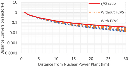
The DCFs for all scenarios show a similar trend as the reduction of relative concentration $\mathit{\chi }/\mathit{Q}$(the ratio of the relative concentration at 1 km as one) shown in the red line. In other words, regardless of the scenario, the effect of the relative concentration, i.e. the effect of dilution by pure diffusion, reduces the effective dose over a long distance. At 30 km, some scenarios show the half reduction ratio compared to the relative concentration. This exceptional accident scenario is the early venting scenario, i.e. FCVS is conducted before 6 hours after scram. However, it should be noted that even the early venting scenario, DCF for each scenario was consistent at the order of magnitude level.

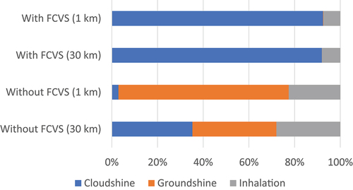
Figure 3 shows the contribution ratios of different exposure pathways for representative accident scenarios with and without FCVS at 1 km and 30 km. The authors have chosen the BWR drywell containment failure (δ4–5) for the ‘Without FCVS’ case, and the BWR containment wet-well release for an in-vessel core melt release with FCVS (φ6–5) for the ‘With FCVS’ case as representative accident scenarios shown in Figure 3. For details on the scenarios, please refer to Table 1 or the figures in the supplementary online material.

Figure 3. The contribution of each exposure pathway to the effective dose without rainfall.

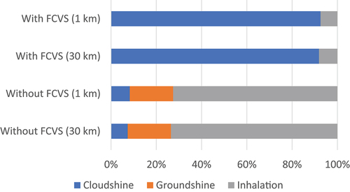
In the case of the scenarios with FCVS, deposition is minimal, with cloudshine making up most of the contribution. On the other hand, in the case without FCVS, the inhalation dose contributes significantly, and groundshine also accounts for about 20% of the total effective dose.

3.2. Results of DCF with rainfall

The DCF $F_p\left(\mathit{x}\right)=F_{\mathit{rain}}\left(\mathit{x}\right)$for each scenario is calculated with rainfall (ground release). The results are shown in Figures 4–6.

Figure 4. DCF for ground release with rainfall (light rain 0.5 mm/h).

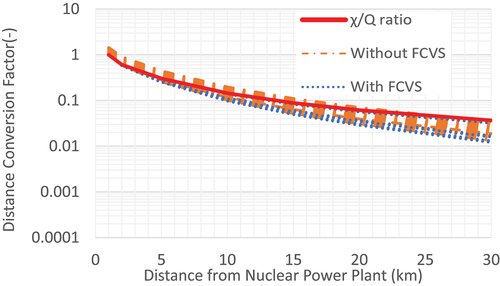
Figure 5. DCF for ground release with rainfall (normal rain 3.8 mm/h).

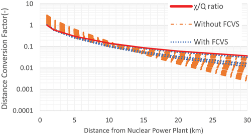
Figure 6. DCF for ground release with rainfall (heavy rain 10 mm/h).

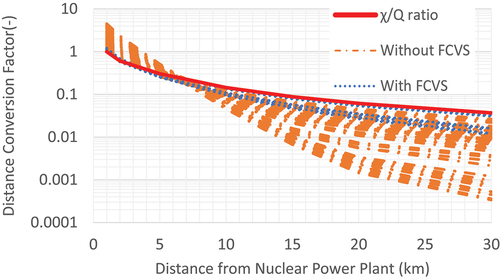
In Figures 4–6, the relative concentration ratios at 1 km and an arbitrary distance are represented by the red line, which corresponds to the same DCF in the case of no rainfall. The blue lines correspond to the scenarios with FCVS, while the orange lines represent those without FCVS depicted in RTM-96.

The DCF in the case of rainfall displays significant variation depending on the severity of the rainfall and the accident scenario. In the case of light rain, the difference between scenarios is not substantial, like the case with no rainfall. However, in the case of normal rainfall, the variation is approximately three-fold at 1 km and nearly an order of magnitude at 30 km. These differences become even more significant with heavy rainfall. This difference in DCF among several accident scenarios suggests that it is difficult for the rainfall case to represent the DCF uniformly across all scenarios using only the relative concentration as the case of no rainfall.

Notably, even when assuming heavy rainfall, the DCF for the scenario with FCVS shows a similar trend to the case without rainfall at short and long distances. This trend in the scenarios with FCVS differs significantly from the original trend of the DCF in RTM-96, which shows a larger value at short distances and a smaller value at long distances compared to the case without rainfall. The original DCF in RTM-96 is presented in Figure 14 and 15 in Section 5, where the differences between RTM-96 and the method in this study are discussed in detail.

This result is because in scenarios with FCVS, the contribution to the effective dose is primarily from noble gases, which are less affected by increased deposition due to rainfall.

An intriguing observation from Figure 7 is that, even under the assumption of rainfall, the contribution from ground shine remains extremely minimal in scenarios that incorporate FCVS. This observation can be attributed to the assumption that aerosols are reduced by a factor of 1000 and elemental iodine by 100 through FCVS suggesting that even in the case of rainfall, the impact of deposition remains limited under these assumptions.

Figure 7. The contribution of each exposure pathway to the effective dose with rainfall.

On the other hand, in scenarios without FCVS, the contribution from groundshine becomes dominant at close distances. However, the washout effect at longer distances removes aerosols, resulting in a less significant contribution from groundshine. In other words, the difference in DCFs by accident scenario depends on whether the scenario has a significant deposition effect, i.e. a scenario with a major aerosol contribution.

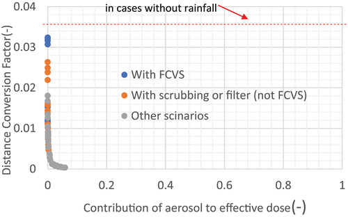
Based on the results above, the analysis focused on the exposure contribution of aerosol nuclides that affect the variation of the DCF for each scenario. The aerosol exposure contribution ratio refers to the percentage of the dose at each distance contributed by nuclides other than noble gases and organic iodine to the effective dose. In this calculation, inorganic iodine was also considered. However, on this occasion, it was assumed that inorganic iodine is a species that can be washed out, so it was in the same group as aerosols. The following discussion will be conducted for each of the following scenarios: scenario with high mitigation effect (scenario with FCVS), scenario with medium mitigation effect (scenarios with suppression pool scrubbing effect, scenario with filters other than venting), and scenario with low mitigation effect (bypass, dry containment release scenario).

Figures 8–10 show the relationship between the aerosol contribution to the effective dose and the DCF for each scenario at 1 km. Blue dots express the scenarios with significant mitigation by FCVS (φ1~φ6 in Table 1). Orange express accident scenarios with moderate mitigating effects, i.e. with suppression pool scrubbing or with a filter other than FCVS (δ5~δ6 and some scenarios in v1~v2 with filter in Table 1). Gray refers to other accident scenarios, including slight mitigation, i.e. dry-well containment release by containment failure.

Figure 8. Relationship between the contribution of aerosol to effective dose and DCF at 1 km (light rain 0.5 mm/h).

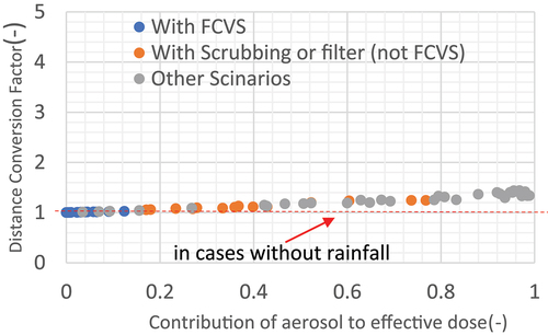
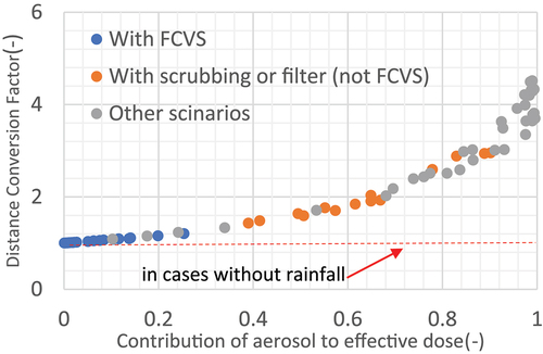
Figure 9. Relationship between aerosol contribution to effective dose and DCF at 1 km (normal rain 3.8 mm/h).

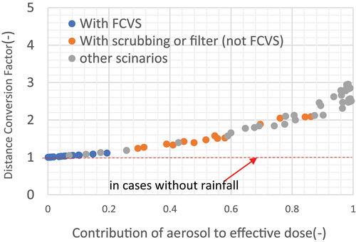
Figure 10. Relationship between aerosol contribution to effective dose and DCF at 1 km (heavy rain 10 mm/h).

As shown in Figures 8–10, the contribution of aerosols to the effective dose was minor for scenarios with FCVS which is expected to have a significant mitigation effect. In comparison, the contribution of aerosols to the effective dose was more significant for scenarios such as bypass and dry containment release which is expected to have little mitigation effect.

At short distances such as 1 km, the DCFs were more prominent for scenarios with a higher proportion of aerosol nuclides to the effective dose. For the small mitigation scenarios such as bypass or dry containment release, in which aerosols contribute more than 80% of the effective dose, the DCF for light rain was almost the same as without rainfall. However, the DCF is up to three for normal rainfall, which means it was about three times higher than that without rainfall. The DCF increased further with heavy rainfall. In other words, for scenarios with a major aerosol contribution to the effective dose, the dose at short distances increases with increasing rainfall.

The DCFs for the moderate mitigation scenarios with pool scrubbing and filter effects other than FCVS also tended to increase as rainfall intensified, but to a lesser extent than for the bypass and dry containment release scenarios.

For the scenarios with FCVS with a minor aerosol contribution, the DCF is almost one, i.e. the same as the DCF without rain. This tendency is the same for light, normal, and heavy rainfall. In other words, for scenarios with a significant noble gas contribution to the effective dose, the exposure does not differ significantly from that without rainfall, regardless of the intensity of the rainfall.

Next, the results of the analysis for long distances are shown. Figures 11–13 show the relationship between the contribution of aerosol to effective dose and the DCF at 30 km.

Figure 11. Relationship between aerosol contribution to effective dose and DCF at 30 km (light rain 0.5 mm/h).

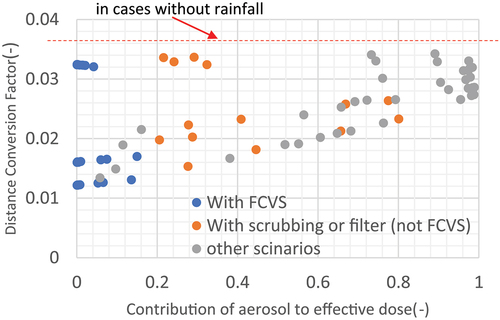
Figure 12. Relationship between aerosol contribution to effective dose and DCF at 30 km (normal rain 3.8 mm/h).

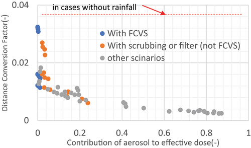
Figure 13. Relationship between aerosol contribution to effective dose and DCF at 30 km (heavy rain 10 mm/h).

There was no significant correlation between the proportion of aerosol contribution and the DCF for light rainfall, which indicates that aerosols were not significantly washed out in the case of light rainfall.

On the other hand, in the case of normal rainfall, the DCFs were smaller at longer distances (e.g. 30 km) for scenarios with a major aerosol contribution. Especially in slight mitigation scenarios such as bypass and dry containment release, where aerosols contribute approximately 80% or more, the DCF is 0.003, i.e. about one-tenth of the dose without rainfall. On the other hand, for most of the scenarios with FCVS, the aerosol contribution to the effective dose was minimal, and the DCF was close to the DCF without rain (about 0.037). In some scenarios such as early release with FCVS scenarios, it was about half of that value due to Kr-88 decay. However, in most scenarios with FCVS, the DCF was almost the same as in the case of no rainfall.

In the case of heavy rainfall, the aerosol component was washed out until it reached 30 km in all scenarios, so the aerosol component becomes minimal in all scenarios. In other words, most of the aerosols were washed out upwind, and what remained 30 km downwind were gaseous radionuclides such as noble gases. In this case, the difference in the DCF between scenarios becomes more pronounced. In scenarios with FCVS, the values remained consistent with those in cases without rainfall. Conversely, in scenarios without FCVS, the values became extremely small because of the large aerosol washout.

These analyses allowed us to quantify the effect of the difference in accident scenarios due to rainfall, which is attributed to the fraction of aerosols in the released nuclides. Specifically, the scenarios with FCVS showed a similar trend to the DCF for no rainfall in all cases. In contrast, scenarios with the pool scrubbing or without FCVS showed some variation from scenario to scenario. For the low mitigation scenarios with a major aerosol contribution, the DCFs were larger at 1 km and smaller at 30 km.

4. Discussion of the models and the various DCFs

This section discusses why the DCF $F_p\left(\mathit{x}\right)$ of most scenarios shows a similar tendency in case without rainfall and a different one in case without rainfall. Then, how to define the DCF, represented among multiple accident scenarios like RTM-96, is discussed. Initially, discussions for the case without rainfall are conducted, followed by examining the case with rainfall.

The effective dose without rainfall can be transformed as follows from Equations (3)(3) ${\chi }_i\left(\mathit{x},\mathit{y},\mathit{z}\right)=\dot{Q_i}\times \mathit{\chi }/\mathrm{Q}\times \mathit{\hspace{0.17em}}exp\left(-{\lambda }_i\mathit{t}\right)\times \mathit{exp}\left(-\mathrm{\Lambda }\frac{x}{u}\right)\times f_F$(3) , (10(10) ${\dot{\chi }}_{\mathit{i},\mathit{D}}\left(\mathit{x},\mathit{y}\right)={\chi }_i\left(\mathit{x},\mathit{y},0\right)\times \left(V_d+V_R\right)$(10) ), (11(11) $H_{\mathit{CS}}=\sum _i{K}_i^{\mathit{CS}}{\chi }_i$(11) ), (12(12) $H_{\mathit{IH}}=\sum _i{K}_i^{\mathit{IH}}{\chi }_i$(12) ), (13(13) $H_{\mathit{GS}}=\sum _i{K}_i^{\mathit{GS}}{\dot{\chi }}_{\mathit{i},\mathit{D}}$(13) ) and (14(14) $H_{\mathit{p}}^S\left(\mathit{x}\right)=H_{\mathit{CS}}+H_{\mathit{GS}}+H_{\mathit{IH}}$(14) ).³ The variable $\mathit{t}$ is the sum of the time from the scram to the release, $t_{\mathit{rel}}$, and the time from the release to the arrival of the plume at the residential location, $\frac{x}{u}$.

(18) $H_{\mathit{norain}}\left(\mathit{x}\right)={\left(\mathit{\chi }/Q\right)}_x\times \sum _{i}exp\left(-{\lambda }_i\mathit{t}\right)\times Q_i\times \left(K_i^{\mathit{CS}}+K_i^{\mathit{IH}}+K_i^{\mathit{GS}}\right)={\left(\mathit{\chi }/Q\right)}_x\times \sum _i\mathit{exp}\left(-{\lambda }_i{t}_{\mathit{rel}}\right)\mathit{exp}\left(-{\lambda }_i\frac{x}{u}\right)\times Q_i\times \left(K_i^{\mathit{CS}}+K_i^{\mathit{IH}}+K_i^{\mathit{GS}}\right)$(18)

The $\mathit{\chi }/\mathit{Q}$ is a relative air concentration that depends on distance but does not depend on nuclides. Therefore, it can be considered almost independent of the accident scenario. On the other hand, following each term on the right side of the above equation is a nuclide-dependent coefficient, which depends on the accident scenario.

(19) $\sum _i\mathit{\hspace{0.17em}}\mathit{exp}\left(-{\lambda }_i{t}_{\mathit{rel}}\right)\mathit{exp}\left(-{\lambda }_i\frac{x}{u}\right)\times Q_i\times {\left(\mathit{Ki}\mathit{CS}+K_i^{\mathit{IH}}+K_i^{\mathit{GS}}\right)}_{\mathit{i}}\mathit{\hspace{0.17em}}$(19)

The only term in the term (19) that depends on both nuclide and distance is the decay term $\exp \left(-{\lambda }_i\frac{x}{u}\right)$ during atmospheric transport. The effect of the decay term during atmospheric transport is seen in the case of accident scenarios such as early venting scenarios where the effect of very short-lived nuclides, i.e. Kr-88, is dominant. In most accident scenarios, the released nuclides do not decay much for a few hours during atmospheric transport; thus,

(20) $exp\left(-{\lambda }_i\frac{x}{u}\right)\cong 1$(20)

In other words, in most scenarios, the effect of the decay term can be ignored when calculating the DCF $F_p^{\mathit{DIST}}\left(\mathit{x}\right)$. Therefore, the following approximation holds.

(21) $\begin{array}{cc}\mathit{\hspace{0.17em}}& F_{\mathit{norain}}\left(\mathit{x}\right)=\frac{{\mathit{H}}_{\mathit{norain}}\left(\mathit{x}\right)}{H_{\mathit{norain}}\left(1\right)}\\ \mathit{\hspace{0.17em}}& \cong {\left(\frac{\chi }{Q}\right)}_{\mathit{x}}/{\left(\frac{\chi }{Q}\right)}_{1\mathit{km}}\times \frac{{\sum }_i{Q}_i\times \left(K_i^{\mathit{CS}}+K_i^{\mathit{IH}}+K_i^{\mathit{GS}}\right)}{{\sum }_i{Q}_i\times \left(K_i^{\mathit{CS}}+K_i^{\mathit{IH}}+K_i^{\mathit{GS}}\right)}\\ \mathit{\hspace{0.17em}}& ={\left(\frac{\chi }{Q}\right)}_{\mathit{x}}/{\left(\frac{\chi }{Q}\right)}_{1\mathit{km}}\end{array}$(21)

This approximation is conservative because it assumes that the radioactivity does not decay during atmospheric transport and reaches the inhabitant points with the radioactivity at the time of release. By applying this approximation, in the case of no rainfall, the DCF can be regarded as dependent on diffusion but independent of the accident scenario. Thus, by calculating the ratio of relative concentrations $\mathit{\chi }/\mathit{Q}$ at 1 km and $\mathit{\chi }/\mathit{Q}$ at any other distance, a scenario-independent DCF can be defined. The approximation (21) holds for other wind speeds and release height without rainfall. Hence, the DCF applicable to all scenarios, denoted as $\mathit{F}{ }_{\mathit{norain}}^{\prime }\left(\mathit{x}\right)$ can be defined by the following formula because of the discussion above.

(22) $\mathit{F}{ }_{\mathit{no}\mathit{rain}}^{\prime }\left(\mathit{x}\right)={\left(\frac{\chi }{Q}\right)}_{\mathit{x}}/{\left(\frac{\chi }{Q}\right)}_{1\mathit{km}}$(22)

Subsequently, considerations regarding the case with rainfall will be presented. The result of the case with rainfall, in which the trend differs between scenarios with a major aerosol contribution and those with a major gas contribution can be interpreted using a formula for derivation of the DCF.

4.1. Scenarios in which gas contribution to the effective dose is major

If the nuclides of the aerosol component are considered small, the effective dose with rainfall is expressed as follows. The terms including the washout coefficient and the groundshine term can be neglected for the gas component.

(23) $H_{\mathit{rain}}\left(\mathit{x}\right)={\left(\mathit{\chi }/Q\right)}_x\times \sum _i\mathit{exp}\left(-{\lambda }_i{t}_{\mathit{rel}}\right)\mathit{exp}\left(-{\lambda }_i\frac{x}{u}\right)\times Q_i\times \left(K_i^{\mathit{CS}}+K_i^{\mathit{IH}}\right)$(23)

The $\mathit{\chi }/\mathit{Q}$ can be considered almost independent of the accident scenario discussed above. On the other hand, following each term on the right side of the above equation, shown as Equation 24(24) $H_i=\sum _i\mathit{exp}\left(-{\lambda }_i{t}_{\mathit{rel}}\right)\mathit{exp}\left(-{\lambda }_i\frac{x}{u}\right)\times Q_i\times {\left(\mathit{Ki}\mathit{CS}+K_i^{\mathit{IH}}+K_i^{\mathit{GS}}\right)}_{\mathit{i}}\mathit{\hspace{0.17em}}$(24) , is a nuclide-dependent coefficient. Therefore, this depends on the accident scenario.

(24) $H_i=\sum _i\mathit{exp}\left(-{\lambda }_i{t}_{\mathit{rel}}\right)\mathit{exp}\left(-{\lambda }_i\frac{x}{u}\right)\times Q_i\times {\left(\mathit{Ki}\mathit{CS}+K_i^{\mathit{IH}}+K_i^{\mathit{GS}}\right)}_{\mathit{i}}\mathit{\hspace{0.17em}}$(24)

The only term in Equation 24(24) $H_i=\sum _i\mathit{exp}\left(-{\lambda }_i{t}_{\mathit{rel}}\right)\mathit{exp}\left(-{\lambda }_i\frac{x}{u}\right)\times Q_i\times {\left(\mathit{Ki}\mathit{CS}+K_i^{\mathit{IH}}+K_i^{\mathit{GS}}\right)}_{\mathit{i}}\mathit{\hspace{0.17em}}$(24) that depends on both nuclide and distance is the decay term $\mathit{exp}\left(-{\lambda }_i\frac{x}{u}\right)$　during atmospheric transport. As discussed for the no rainfall case, while there is a contribution in scenarios such as early venting, it is only of a factor of two contribution, and it is conservative to determine the DCF without considering this term.

Therefore, the following approximation holds.

(25) $F_{\mathit{rain}}\left(\mathit{x}\right)=\frac{{\mathit{H}}_{\mathit{rain}}\left(\mathit{x}\right)}{H_{\mathit{no}\mathit{rain}}\left(1\right)}\cong \frac{{\left(\mathit{\chi }/Q\right)}_x}{{\left(\mathit{\chi }/Q\right)}_{1\mathit{km}}}\times \left(\frac{{\sum }_j{Q}_j\times \left(K_j^{\mathit{CS}}+K_j^{\mathit{IH}}\right)}{{\sum }_j{Q}_j\times \left(K_j^{\mathit{CS}}+K_j^{\mathit{IH}}\right)}\right)=\frac{{\left(\mathit{\chi }/Q\right)}_x}{{\left(\mathit{\chi }/Q\right)}_{1\mathit{km}}}$(25)

From this, even during rainfall, the DCF is almost equivalent to that without rainfall. In other words, this explains why the DCFs show the same trend as in the case without rainfall, even when rainfall is considered in the scenario in which the gas component is dominant. Hence, the DCF applicable to multiple scenarios, denoted as $\mathit{F}{ }_{\mathit{rain}}^{\prime }\left(\mathit{x}\right)$can be defined by the following formula, because of the discussion above.

(26) $\mathit{F}{{\mathit{ }}^{\mathrm{\prime }}}_{\mathit{rain}}\left(\mathit{x}\right)=\mathit{F}{ }_{\mathit{no}\mathit{rain}}^{\prime }\left(\mathit{x}\right)=\frac{{\left(\mathit{\chi }/Q\right)}_x}{{\left(\mathit{\chi }/Q\right)}_{1\mathit{km}}}$(26)

The scenarios with FCVS are those in which gas contribution to the effective dose is major. Thus, it is considered appropriate to consider the DCF with $\mathit{\chi }/\mathit{Q}$ ratio, which is the same as the case of no rainfall.

4.2. Scenarios in which aerosol components’ contribution to dose is major

In this section, the DCF for a given accident scenario is formulated in the approximation that the effect of decay during atmospheric transport, as specified in 3.2, is small. When the contribution of the nuclides in the gas component is small,

(27) $F_{\mathit{rain}}\left(\mathit{x}\right)=\frac{{\mathit{H}}_{\mathit{rain}}\left(\mathit{x}\right)}{H_{\mathit{no}\mathit{rain}}\left(1\right)}\cong \frac{{\left(\mathit{\chi }/Q\right)}_x}{{\left(\mathit{\chi }/Q\right)}_{1\mathit{km}}}\times \frac{exp\left(-\mathrm{\Lambda }\frac{x}{u}\right)}{1}\times \left(\frac{{\sum }_i{Q}_i\times \left(K_i^{\mathit{CS}}+K_i^{\mathit{IH}}\right)+\left(V_d+V_R\right)\times {\sum }_i{Q}_i\times K_i^{\mathit{GS}}}{{\sum }_i{Q}_i\times \left(K_i^{\mathit{CS}}+K_i^{\mathit{IH}}\right)+V_d\times {\sum }_i{Q}_i\times K_i^{\mathit{GS}}}\right)$(27)

where, for short distances, i.e. close to 1 km, the terms for the effect of atmospheric transport and the term for the effect of washout, which depends on distance, are respectively.

(28) $\frac{{\left(\mathit{\chi }/Q\right)}_x}{{\left(\mathit{\chi }/Q\right)}_{1\mathit{km}}}\cong 1,\frac{exp\left(-\mathrm{\Lambda }\frac{x}{u}\right)}{1}\cong 1,$(28)

while the terms representing the effect of each nuclide weighted by the dose conversion coefficient and deposition rate are,

(29) $\left(\frac{{\sum }_i{Q}_i\times \left(K_i^{\mathit{CS}}+K_i^{\mathit{IH}}\right)+\left(V_d+V_R\right)\times {\sum }_i{Q}_i\times K_i^{\mathit{GS}}}{{\sum }_i{Q}_i\times \left(K_i^{\mathit{CS}}+K_i^{\mathit{IH}}\right)+V_d\times {\sum }_i{Q}_i\times K_i^{\mathit{GS}}}\right)>1$(29)

Thus, at short distances, $F_{\mathit{rain}}\left(\mathit{x}\right)$ >1, indicating that the degree of exposure is greater in the presence of rainfall than without rainfall. When the degree of rainfall is weak, $V_R\cong 0$, this term is almost equal to one, but when the degree of rainfall is strong, the value of this term is larger than one.

The term representing the effect of each nuclide weighted by the dose conversion coefficient and deposition rate becomes larger because there is a groundshine effect $V_R\times \sum _i{Q}_i\times K_i^{\mathit{GS}}$ due to wet deposition of the aerosols.

A key situation where the impact of groundshine is at short distances pronounced, leading to a significant increase in $F_{\mathit{rain}}\left(\mathit{x}\right)$arises during heavy rainfall and $V_R$ is extremely large in Equation 29.(29) $\left(\frac{{\sum }_i{Q}_i\times \left(K_i^{\mathit{CS}}+K_i^{\mathit{IH}}\right)+\left(V_d+V_R\right)\times {\sum }_i{Q}_i\times K_i^{\mathit{GS}}}{{\sum }_i{Q}_i\times \left(K_i^{\mathit{CS}}+K_i^{\mathit{IH}}\right)+V_d\times {\sum }_i{Q}_i\times K_i^{\mathit{GS}}}\right)>1$(29) Additionally, if the evaluation target shifted to the bone marrow dose, $F_{\mathit{rain}}\left(\mathit{x}\right)$ would be large. This tendency is due to the bone marrow dose often showing a greater susceptibility to groundshine’s effect than inhalation.

Conversely, if the effect of groundshine is relatively small, this term will be almost equal to 1, and the DCF will be about the same as in the absence of rainfall. This situation shows the case when the degree of rainfall is small and there is little deposition (i.e. $V_R$≅0) or when the evaluation is based on thyroid dose, which often concerns inhalation effects more than external exposure. On the other hand, the effect of washout is not negligible at long distances. Equation 30(30) $\frac{exp\left(-\mathrm{\Lambda }\frac{x}{u}\right)}{1}\ll 1$(30) explains why the value of $F_{\mathit{rain}}\left(\mathit{x}\right)$ is extremely small at long distances.

(30) $\frac{exp\left(-\mathrm{\Lambda }\frac{x}{u}\right)}{1}\ll 1$(30)

Based on these considerations, the authors discuss DCFs which are applicable to multiple scenarios in the case of rainfall so that they can be used promptly in an emergency.

In most accident scenarios without FCVS, the contribution of aerosols is larger. Thus, DCF is large at short distances and small at long distances because of washout. However, the DCF varies in accident scenarios because of the differences in dominant exposure pathway. Therefore, the authors suggest that the largest DCF for all scenarios other than FCVS be conservatively defined as the representative value that can be applied across multiple accident scenarios as follows.

(31) $F_{\mathit{rain}}^{\prime }\left(\mathit{x}\right)=\mathit{Max}(H_{\mathit{rain}}\left(\mathit{x}\right)/H_{\mathit{no}\mathit{rain}}\left(1\right))$(31)

This approach means taking the maximum DCF for all scenarios at each specific distance $\mathit{x}$. Specifically, at shorter distances, the DCF of scenarios where aerosol contribution is particularly significant and deposition is severe (i.e. scenarios with significant groundshine) will be adopted. Conversely, at longer distances, the DCF of scenarios where washout has not been as pronounced will be chosen.

5. Comparison of DCFs calculated by this method and DCFs defined in RTM-96

Using the method outlined in Section 4, representative DCFs $F_{\mathit{norain}}^{\prime }\left(\mathit{x}\right)$ and $F_{\mathit{rain}}^{\prime }\left(\mathit{x}\right)$that can be applicable to multiple accident scenarios, corresponding to the effective dose, were calculated for this study. These were compared with the DCFs corresponding to the bone marrow dose defined in RTM-96.

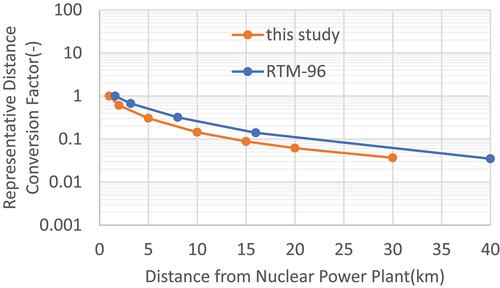
Figure 14 shows that, in the case without rainfall, the DCFs of both this study and RTM-96 decrease with distance in almost the same manner. The slight difference is due to the reference point (1 km or 1 mile). If the reference points are aligned, the two are almost identical.⁴ It is worth noting that while RTM-96 only describes the values, this study presents the DCF as a formula. Therefore, unlike RTM-96, it allows for more flexible applications, such as adapting to various wind speeds.

Figure 14. Comparison of DCF at varying distances from Nuclear Power Plant when DCF is 1 at 1 mile for RTM-96 and 1 at 1 km for this study (without rainfall).

Next, Figure 15 shows that when there is rainfall, the DCFs of this study and those defined in RTM-96 differ. At short distances, the DCFs of the RTM-96 are several times larger than those of this study. One major reason is that the DCFs of RTM-96 are designed to correspond to the calculation of bone marrow doses, which are more sensitive to rainfall and groundshine. On the other hand, at long distances, the DCFs in this study (even without FCVS) are larger than those of the RTM-96. This is because the DCFs without FCVS in this study are defined as the maximum value of the DCFs for all scenarios without FCVS. In other words, the DCFs of RTM-96 tend to be like those of the ‘scenarios with a large contribution of aerosol components’ calculated in this study. In contrast, the representative DCFs in this study are calculated considering some scenarios with relatively small aerosol contribution in scenarios without FCVS. Even in scenarios without FCVS, there are cases where partial mitigation is successful, resulting in some aerosol removal, and the effects of gaseous and aerosol releases become equally significant. In these scenarios, at long distances, the effect of washout in rainy conditions is less effective compared to scenarios where aerosols contribute almost 100%. In the method proposed in this study, which considers the maximum DCF approach, the impact of scenarios where washout is less effective is also considered. Therefore, the DCF values at long distances are higher than those in RTM-96. Adopting this approach makes it possible to prevent the underestimation of dose at long distances in scenarios where partial mitigation is successful, particularly in rainfall cases.

Figure 15. Comparison of DCF at varying distances from Nuclear Power Plant when DCF is 1 at 1 mile for RTM-96 and 1 at 1 km for this study (with rainfall).

The differences in features between RTM-96 and the DCF of this study are summarized in Table 2.

Table 2. Comparison between DCF of RTM-96 and this study.

	This study	RTM-96
Reference distance	1 km	1 mile
metric	Effective dose	Bone marrow dose or thyroid dose
DCF formula in case without rain	${\mathit{F}}_{\mathit{no}\mathit{rain}}^{{ }^{\mathbf{\prime }}}\left(\mathit{x}\right)$=${\left(\frac{\mathit{\chi }}{\mathit{Q}}\right)}_{\mathit{x}}/{\left(\frac{\mathit{\chi }}{\mathit{Q}}\right)}_{1\mathit{km}}$	Only the DCF values are recorded.
DCF formula in case with rain	In scenarios with FCVS, ${\mathit{F}}_{\mathit{rain}}^{{ }^{\mathbf{\prime }}}\left(\mathit{x}\right)$$={\left(\frac{\chi }{Q}\right)}_{\mathit{x}}/{\left(\frac{\chi }{Q}\right)}_{1\mathit{km}}$ In scenarios without FCVS, $F_{\mathit{rain}}^{\prime }(\mathit{x})=\mathit{Max}(H_{\mathit{rain}}(\mathit{x})/H_{\mathit{no}\mathit{rain}}(1))$	Only the DCF values are recorded. Consideration of FCVS and classification based on the contribution of aerosols are not made.

6. Conclusion

The variation in dose with distance was analyzed for each accident scenario, considering both conditions: with and without rainfall. The variation in dose with distance was represented using a parameter called DCF, which is the ratio between the dose at 1 km and the effective dose at an arbitrary location. This study expands the discussion on FCVS, which is not covered in RTM-96, in addition to the accident scenarios addressed in RTM-96. By establishing a reduction factor $F_i^{\mathit{RDF}}$ corresponding to FCVS, the authors have newly added accident scenarios that consider FCVS. Furthermore, this study focuses on the contribution of aerosols to dose and quantitatively evaluates the impact of various levels of rainfall on variation in dose with distance.

It was found in this study that the characteristics of DCF differ depending on the presence or absence of FCVS during rainfall. Since RTM-96 does not consider FCVS, a DCF that considers FCVS has newly established. Furthermore, the authors have not only presented the values of DCF, but also showed a calculation formula of DCF. The specific findings regarding the presence or absence of FCVS, and the impact of the presence and intensity of rainfall, are as follows.

In the case without rainfall, it is possible to approximate the DCF, by the ratio of relative concentration $\mathit{\chi }/\mathit{Q}$ at 1 km and an arbitrary distance using an approximation that does not consider the effect of depletion during atmospheric transport, and the difference between scenarios becomes small. The results obtained are based on the assumptions of wind speed and atmospheric stability used in this study. However, it is suggested that these findings can be applicable to other wind speed and levels of atmospheric stability. Therefore, in the case without rainfall, the authors propose that the ratio of relative concentrations be defined as a DCF applicable to all scenarios, including those with FCVS.

In the case with light rainfall, the trend is almost the same as in the no rainfall case. However, in the case of normal or heavy rainfall, dose as a function of distance varies significantly among accident scenarios because the contribution of aerosols differs among accident scenarios. The differences in characteristics for each scenario in the case with rainfall are as follows.

For the scenarios with FCVS, where the gas component has a large influence, the trend was almost the same even in case with rainfall, as in case without it. In particular, the scenarios with FCVS did not differ from the case without rainfall, even with the assumption of heavy rainfall. Therefore, in scenarios with FCVS, it is appropriate to define the representative DCF as the same, even in the presence of rainfall, as in cases without it.

For the scenarios without FCVS, i.e. the accident scenario with a large aerosol contribution to effective dose, such as the containment failure scenario, the DCF increases at short distances in case with rainfall. The DCF decreases at long distances, but the extent of this effect varies significantly depending on the accident scenario. In other words, the scenarios considered originally in the RTM-96 other than FCVS are non-conservative in some scenarios if it is assumed that the presence of rainfall reduces the dose at long distances. Therefore, the authors propose that the maximum value of the DCF for all scenarios except FCVS be used as the representative DCF in the presence of rainfall. The calculations using this method, especially in the presence of rainfall, show a significant difference in trend from the DCFs in the RTM-96.

As a future work, it is necessary to expand the calculation based on this study’s method considering the FCVS for thyroid dose and bone marrow dose, which were originally targeted in RTM-96, and to clarify the differences in characteristics compared to the effective dose-based DCF addressed in this study. Differences probably emerge between the DCF based on effective dose and DCF targeting thyroid dose or bone marrow dose, especially in case of rainfall. Therefore, while the DCF values from this study can be used for practical purposes in calculating effective doses, it is recommended to refer to the DCFs listed in RTM-96 when using DCFs for thyroid and bone marrow doses, currently.

Acknowledgments

The authors are deeply grateful to Nuclear Regulation Authority’s Technical Adviser, Mr. Toshimitsu Homma, and Dr. Yutaka Abe for the guidance on the paper. The authors also greatly appreciate the support from Dr. Chihiro Suzuki. Furthermore, the authors would like to thank Dr. Hiroki Okajima for his assistance in creating the programming for the calculation used in this study.

Disclosure statement

No potential conflict of interest was reported by the author(s).

Supplementary material

Supplemental data for this article can be accessed online at https://doi.org/10.1080/00223131.2024.2313551

Notes

1. In Equation 2(2) $\dot{Q_i}=Q_i^{\mathit{INV}}\times F_i^{\mathit{CRF}}\times F_i^{\mathit{RDF}}\times F^{\mathit{EF}}\mathit{\hspace{0.17em}}$(2) , the values were represented ‘per hour,’ but in Equation 3(3) ${\chi }_i\left(\mathit{x},\mathit{y},\mathit{z}\right)=\dot{Q_i}\times \mathit{\chi }/\mathrm{Q}\times \mathit{\hspace{0.17em}}exp\left(-{\lambda }_i\mathit{t}\right)\times \mathit{exp}\left(-\mathrm{\Lambda }\frac{x}{u}\right)\times f_F$(3) , the values converted ‘per second’ were used.

2. When the weather condition is no rain, the washout coefficient is 0.

3. The washout coefficient is zero since the weather condition is no rain and $f_F\cong 1$ in D stability.

4. This is described in Table S3 and Figure S11 of the supplementary online material.

References

- McKenna TJ. Protective action recommendations based upon plant conditions. J Hazard Mater. 2000;75:145–164. doi: 10.1016/S0304-3894(00)00177-1
- McKenna TJ, Trefethen J, Gant K, et al. Response technical manual: RTM-96, Washington, DC: U.S. Nuclear Regulatory Commission; 1996, (NUREG/BR-0150) Volume 1, Revision 4.
- U.S. Environmental Protection Agency (EPA). Manual of protective action guides and protective actions for nuclear incidents. Washington, DC: U.S. Environmental Protection Agency; 2017. (EPA-400/R-17/001).
- Carless TS, Talabi SM, Fischbeck PS. Risk and regulatory considerations for small modular reactor emergency planning zones based on passive decontamination potential. Energy. 2019;167:740–756. doi: 10.1016/j.energy.2018.10.173
- Mitrakos D. Radiological impact and emergency zones for small iPWR with different approaches for source term calculation. Prog Nucl Energy. 2022;145:104123. doi: 10.1016/j.pnucene.2022.104123
- Ulimoen M, Berge E, Klein H et al. Comparing model skills for deterministic versus ensemble dispersion modelling: The Fukushima Daiichi NPP accident as a case study. Sci Total Environ. 2022;806:150128. doi: 10.1016/j.scitotenv.2021.150128
- Niisoe T. An iterative application of the green’s function approach to estimate the time variation in 137Cs release to the atmosphere from the Fukushima Daiichi nuclear power Station. Atmos Environ. 2021;254:118380. doi: 10.1016/j.atmosenv.2021.118380
- Ramsdell JV, Athey GF, McGuire SA, et al. RASCAL 4: description of models and methods. Washington, DC: U.S. Nuclear Regulatory Commission; 2012. (NUREG-1940).
- Zhao Y, Zhang L, Tong J. Development of rapid atmospheric source term estimation system for AP1000 nuclear power plant. Prog Nucl Energy. 2015;81:264–275. doi: 10.1016/j.pnucene.2015.02.008
- IAEA. Generic assessment procedures for determining protective actions during a reactor accident. Vienna: International Atomic Energy Agency; 1997. (IAEA-TECDOC-955).
- Athey GF, Sjoreen AL, Ramsdell JV, et al. RASCAL version 2.1 user’s guide. Washington, DC: U.S. Nuclear Regulatory Commission; 1994. (NUREG/CR-5247 Volume 1, Revision 2).
- Athey GF, Sjoreen AL, Ramsdell JV, et al. RASCAL version 2.1 workbook. Washington, DC: U.S. Nuclear Regulatory Commission; 1994. (NUREG/CR-5247 Volume 2, Revision 2).
- Jacquemain D, Guentay S, Basu S, et al. OECD/NEA/CSNI status report on filtered containment venting. OECD/NEA;2014, (NEA-CSNI-R-2014-7)
- Ebrahimgol H, Aghaie M. Evaluation of Filtered Containment Venting System (FCVS) effects on severe accident of a WWER1000 plant. Ann Nucl Energy. 2023;181:64–74. doi: 10.1016/j.anucene.2022.109522
- IAEA, Preparedness and response for a nuclear or radiological emergency. Vienna: International Atomic Energy Agency, 2015, (IAEA SAFETY STANDARDS SERIES No. GSR Part 7)
- Dose estimates to be referred to in the formulation of nuclear emergency preparedness measures [Internet]. Japan: Nuclear Regulatory Authority;2018 Oct 17 [cited 2023 Jun 22] Available from: https://www.nra.go.jp/data/000249587.pdf
- U.S. Nuclear Regulatory Commission. Reactor safety study: an assessment of accident risks in U.S. Commercial nuclear power plants, executive summary. Washington, DC: Nuclear Regulatory Commission; 1975. (WASH-1400).
- Soffer L, Burson SB, Ferrell CM, et al. Accident source terms for light-water nuclear power plants. Washington, DC: U.S. Nuclear Regulatory Commission; 1995. (NUREG-1465).
- McKenna TJ, Giitter JG. Source term estimation during incident response to severe nuclear power plant accidents. Washington, DC: U.S. Nuclear Regulatory Commission; 1988. (NUREG-1228).
- NSC. Meteorological guidelines for safety analysis of nuclear power reactor facilities [in Japanese]; 1982(revised in 2001)
- Atomic Energy Society of Japan. Code of practice for probabilistic risk assessment of nuclear power plants (level 3 PRA version);2018. (AESJ-SC-P010:2018)
- McGuire SA, Ramsdell JV, Athey GF. RASCAL 3.0.5: description of models and methods. Washington, DC: U.S. Nuclear Regulatory Commission; 2007. (NUREG-1887).
- U.S. Nuclear Regulatory Commission. Severe accident risks: an assessment for five U.S. Nuclear power plants. Washington, DC: U.S. Nuclear Regulatory Commission; 1990. (NUREG-1150, vol. 1).
- Nosek AJ, Bixler N. MACCS theory manual. Albuquerque: Sandia National Laboratories; 2021. (SAND2021-11535).
- Sprung JL, Rollstin JA, Helton JC et al. Evaluation of severe accident risks: quantification of major input parameters. Albuquerque: Sandia National Laboratories; 2021. (SAND86-1309, NUREG/CR-4551).
- Terms related to rain [internet]. Japan: Japan Meteorological Agency; [cited 2023 Jun 12] Available from: https://www.jma.go.jp/jma/kishou/know/yougo_hp/kousui.html
- Eckerman KF, Ryman JC. External exposure to radionuclides in air, water, and soil. Washington, DC: U.S. Environmental Protection Agency; 1993. (EPA-402-R-93-081).
- Eckerman KF, Wolbarst AB, Richardson ACB. Limiting values of radionuclide intake and air concentration and dose conversion factors for inhalation, submersion, and ingestion. Washington, DC: U.S. Environmental Protection Agency; 1988; (EPA-520/1-88-020).