Accounting for Missing Correlation Coefficients in Fixed-Effects MASEM

ABSTRACT

Meta-analytic structural equation modeling (MASEM) is increasingly applied to advance theories by synthesizing existing findings. MASEM essentially consists of two stages. In Stage 1, a pooled correlation matrix is estimated based on the reported correlation coefficients in the individual studies. In Stage 2, a structural model (such as a path model) is fitted to explain the pooled correlations. Frequently, the individual studies do not provide all the correlation coefficients between the research variables. In this study, we modify the currently optimal MASEM-method to deal with missing correlation coefficients, and compare its performance with existing methods. This study is the first to evaluate the performance of fixed-effects MASEM methods under different levels of missing correlation coefficients. We found that the often used univariate methods performed very poorly, while the multivariate methods performed well overall.

KEYWORDS:

• Meta-analytic structural equation modeling
• meta-analysis
• missing data
• TSSEM

Accounting for missing correlation coefficients in fixed-effects MASEM

Meta-analytic structural equation modeling (MASEM) is a technique of pooling correlation coefficients of a set of variables from several independent samples, in order to fit structural equation models on the pooled matrix (see Cheung, 2015a; Jak, 2015). Researchers are increasingly interested in how MASEM can be used to advance theories by synthesizing existing findings (Bergh et al., 2016). The increasing popularity is demonstrated through a recently published special issue of the journal Research Synthesis Methods devoted to the methodological and statistical development of MASEM (Cheung & Hafdahl, 2016).

MASEM essentially comprises two stages. In Stage 1, a pooled correlation matrix is estimated. In Stage 2, a structural model (such as a path model) is fitted to explain the pooled correlations. One of the many nice aspects of MASEM is that the primary studies do not have to include all variables of interest (Viswesvaran & Ones, 1995). For example, Topa & Moriano (2010) gathered correlation coefficients between social norms, attitudes, perceived control, smoking intention, and smoking from 35 published studies, obtaining a total of 217 correlations. A synthesis of the observed correlations across studies provided a pooled correlation matrix of the five variables. By fitting a path model to the pooled correlation matrix, they tested how well the theory of planned behavior could predict smoking behavior. Among other results, they found that social norms better predicted smoking intentions and smoking than attitudes. These researchers obtained 217 correlation coefficients, while with complete data one would extract 10 correlation coefficients per study, leading to 350 correlation coefficients. The missing correlation coefficients may be the result of variables not being included in the study, or of nonreporting correlation coefficients between variables that were included in the study.

When a primary study includes a variable, but does not report all correlations or covariances of this variable with the other variables, this leads to difficulties when applying some MASEM-methods. Specifically, it leads to problems when using methods that pool the data on the variable level, such as fixed-effects two-stage structural equation modeling (TSSEM, Cheung & Chan, 2005). As TSSEM is found to outperform other methods in several aspects, and TSSEM is increasingly applied by meta-analysts, it is essential to adapt TSSEM to handle missing correlation coefficients.

One aim of this article is to show how fixed-effects TSSEM can be used when some correlation coefficients are missing, and to compare the new approach with existing approaches using simulated data with varying amounts of missing data. The new approach will be compared to the original TSSEM approach and two other MASEM-methods that accommodate missing correlations coefficients, being the GLS approach (Becker, 2009) and the univariate approach (Viswesvaran & Ones, 1995).

The second aim of this study is to compare the performance of univariate and multivariate models in the presence of missing correlation coefficients. MASEM is increasingly applied in many fields, such as personality (Connelly & Chang, 2016), health psychology (Cheung & Hong, 2017), medicine (Rich, Brandes, Mullan, & Hagger, 2015), management (Mesmer-Magnus, Asencio, Seely, & DeChurch, 2015), and international business (Tang & Cheung, 2016), but most researchers pool correlation coefficients using (sub-optimal) univariate methods (Hedges & Olkin, 1985; Schmidt & Hunter, 2015). Univariate methods ignore that correlation coefficients within a study are based on the same sample, and that they are therefore not independent. Ignoring this dependency has been found to lead to incorrect results (Cheung & Chan, 2005; Riley, 2009). Multivariate methods such as TSSEM and the GLS approach, that account for within-study dependency of effect-sizes, may improve the performance of the analyses.

One common criticism on the univariate models is that they treat the pooled correlation matrix as if it was a covariance matrix in fitting structural equation models (Cheung, 2015a; Cheung & Chan, 2005). Correlation matrices can be correctly analyzed by imposing appropriate constraints on the model implied variances (Bentler & Lee, 1983). It is of practical interest to see whether the univariate models can be modified to improve their statistical performance. If the modified approach performs as well as multivariate approaches, applied researchers may use the modified univariate models which are arguably easier to implement than the multivariate models. Before presenting the new method to account for missing correlation coefficients and the simulation study, we will elaborate on the occurrence of missing correlation coefficients and explain how the currently available methods handle missing coefficients.

Missing data in MASEM

Missing data in MASEM can occur at different levels: at the study level, at the variable level, and at the coefficient level. At the study level, missing data may occur because not all executed studies may be included in the review. It is a well-known problem that studies with favorable outcomes are easier to publish than studies with unfavorable outcomes, known as publication bias (Rothstein, Sutton, & Borenstein, 2006). Publication bias is a large problem, and various researchers work on methods to attack this problem (Guan & Vandekerckhove, 2016; Simonsohn, Nelson, & Simmons, 2014; van Assen, van Aert, & Wicherts, 2016).

Within available studies, there may be missing data at the variable level, meaning that not all variables of interest were included in the study. Possible reasons are that: (1) the variable was outside the scope of the specific study, (2) at that time, a variable was not operationalized yet (for example, “emotional intelligence” or “cyberbullying” are fairly new concepts), (3) the variable did not show interesting effects, and therefore the authors decided not to report anything on this variable (selective reporting; John, Loewenstein, & Prelec, 2012). The effect of missing variables on the performance of a selection of MASEM-methods was evaluated by Furlow & Beretvas (2005).

If a variable was included in the final model, then there may still be missing information at the coefficient level: not all correlation coefficients of the included variables may be reported. This often happens for correlations that were not the main focus of the researchers, like the correlation between two dependent variables in two separate univariate regression analyses, or the correlation between two independent variables in a path model. In a recent review of applications of MASEM by Sheng, Kong, Cortina, & Hou (2016), it appeared that 38.8% of the meta-analyses were hampered by missing correlation coefficients of this kind. In this article, we focus on missingness at the coefficient level, as the impact of this type of missingness on the performance of MASEM-methods has never been evaluated yet.

In the next section, we will briefly explain the univariate method, the GLS method and TSSEM for fixed effects MASEM, and we will indicate how these methods handle missing correlation coefficients.

Existing methods and missing correlation coefficients

All MASEM-methods essentially consist of two stages. In Stage 1, correlation coefficients are pooled across the studies. In Stage 2, a structural model is fitted to explain the pooled correlations. The existing methods for MASEM differ mostly in how the correlations are pooled (Stage 1). Fitting the model at Stage 2 is not well developed for any of the methods, except for TSSEM.

 

 

Univariate MASEM

Although the univariate methods are not recommended in MASEM (Cheung, 2015a; Cheung & Chan, 2005; Cheung & Hafdahl, 2016; Jak, 2015), most researchers still use univariate methods to pool the correlations (Rosopa & Kim, 2016; Sheng et al., 2016). In univariate MASEM, standard univariate meta-analytic techniques are used to pool correlation coefficients (Field, 2001; Hafdahl & Williams, 2009; Hedges & Olkin, 1985; Schmidt & Hunter, 2015). In the Hunter and Schmidt approach, which we will use in this study, the pooled correlation coefficient between the ith and jth variable across the K studies that reported the correlation coefficient is estimated by (1) where n_k is the sample size in a specific study k. Because the correlation coefficients are pooled across studies one by one, using only the information from studies that provided the respective correlation coefficient, missing correlation coefficients do not immediately lead to problems in Stage 1 of the univariate methods.

Univariate pooling of correlation coefficients will result in a pooled correlation matrix in which possibly each correlation is based on a different subset of studies. This pooled correlation matrix is then used as the observed matrix in an SEM-analysis, where the hypothesized structural model is fitted on the pooled correlations. Although missing correlation coefficients do not seem to be a problem in constructing a pooled correlation matrix, several other issues limit the usefulness of the approach. First, within-study dependency across correlation coefficients is not taken into account (as opposed to multivariate methods such as GLS and TSSEM). Second, using different information for each correlation coefficient may lead to nonpositive definite correlation matrices, which cannot be analyzed with structural equation modeling. Third, by using the pooled correlation matrix as the observed matrix, differences in precision of the estimated pooled correlations are ignored. Fourth, as each correlation may be based on a different number of studies, it is unclear which sample size should be used at Stage 2. Fifth, the univariate approach incorrectly treats the pooled correlation matrix as if it was a covariance matrix. Our simulation study will show whether the advantage of handling missing correlation coefficients outweighs these five disadvantages of the univariate approach. In addition, we will evaluate whether evaluating the correlation matrix using the appropriate diagonal constraints, ensuring that the implied variances are one during estimation, will lead to better performance of the univariate approach.

Generalized least squares (GLS)

Generalized least squares (GLS, Becker, 1992, 1995) is a multivariate approach to pool correlation matrices for MASEM. With GLS, the vector of pooled correlation coefficients across studies, , is estimated using (2) where V is a block diagonal matrix with the sampling covariance matrix of the observed correlation coefficients for each study on its diagonal, X is a selection matrix to select which correlation coefficients are present in each study, and r is a vector with the observed correlations in all the studies. For a detailed and accessible description of GLS, readers may refer to Card (2015). With GLS, the correlations are pooled on the coefficient level, which means that missing coefficients in studies are no problem at Stage 1. GLS takes dependency across correlation coefficients into account by weighting the studies’ correlations by the inverse sampling variances and covariances in V. In a study on the effect of missing variables in MASEM, GLS was found to consistently outperform the univariate methods (Furlow & Beretvas, 2005).

GLS is rarely applied by researchers, because there is no dedicated software to conduct the analyses. Researchers will have to write their own programs to implement the approach. An example of a Stage 1 analysis with GLS using R is provided by Jak (2015). At Stage 2, the original GLS approach (Becker, 2009) can only evaluate path models, and not factor models. A practical, and statistically correct, approach is to fit the structural model on the pooled correlation matrix while using the asymptotic covariance matrix of the pooled correlations as weights in WLS-estimation (Cheung & Chan, 2005), similar to TSSEM, which is explained in the next paragraph.

The original TSSEM (OV approach)

Fixed-effects two-stage structural equation modeling (Cheung & Chan, 2005) uses structural equation modeling at both stages of MASEM. The pooled correlation matrix is estimated by fitting a multigroup model in which each study represents a group, and the correlations are constrained to be equal across groups. For each study k with q of the p variables of interest, the multigroup model is (3) where is the p by p common population correlation matrix, Σ_k is the q by q model implied covariance matrix for study k, D_k is a q by q diagonal matrix for study k that accounts for scaling differences (or standard deviations) across the studies, and X_k is a q by p selection matrix to select out missing variables for study k.

Missing variables do not impose any problem in TSSEM, as they are filtered out by X_k, but missing correlations on the coefficient level may lead to nonpositive definite observed correlation matrices, which cannot be analyzed in SEM. As a consequence, for each missing correlation, one of the two variables associated with the correlation has to be treated as missing. For example, if a study included three variables, but r₃₂ is not reported, while r₂₁ and r₃₁ are, either Variable 2 or Variable 3 is deleted to make the observed matrix positive definite again. This leads to a loss of information and counts as the biggest disadvantage of fixed-effects TSSEM.

On the other hand, TSSEM does not have the limitations of the univariate approach, and the user friendly R-package “metaSEM” can be used to fit the models (Cheung, 2015b). In TSSEM, the structural model is fitted to the pooled correlation matrix using weighted least-square estimation with the asymptotic covariance matrix from Stage 1 as the weight matrix W (Cheung & Chan, 2005). These weights ensure that correlation coefficients that are based on more information (on more studies and/or studies with larger sample sizes) get more weight in the estimation of the Stage 2 parameters. The employed WLS-discrepancy function is (4) where is a vector with the lower triangular elements of the estimated pooled correlation matrix from Stage 1, () is a vector with the lower triangular elements of the model implied correlation matrix, and W is the weight matrix containing the inverse of the asymptotic covariance matrix of the elements in . In order to analyze a correlation matrix correctly, the constraint diag()) = diag(I) on the model implied covariance matrix is applied during the estimation (Cheung, 2015a). Minimizing leads to estimates of the model parameters in and a χ² measure of fit.

Using WLS ensures that differences in precision of the pooled correlation coefficients are taken into account, that all types of structural models can be estimated, and that one does not have to specify a specific sample size at Stage 2. The only limitation of TSSEM is therefore that missing correlation coefficients lead to the removal of even more data. This is a problem that we will solve by proposing an adapted version of TSSEM.

The adapted TSSEM (OC approach)

In this study, we propose and evaluate an adapted version of TSSEM that can account for missing correlation coefficients. To differentiate between the original and the new method, we will refer to the original TSSEM as the omitted variable approach (OV approach) and to the new approach as the omitted correlation approach (OC approach). In the OC approach, similar to the OV approach, a multigroup model with equality constraints on the correlation coefficients is used to estimate the pooled correlation matrix. Now, instead of deleting a variable for which a correlation coefficient is missing, for each missing correlation coefficient, we plug in an arbitrary value and free the respective equality constraint on the parameter in the specific study where the coefficient is missing. This leads to an additional estimated parameter for each missing (and consequently plugged in) correlation coefficient. The missing correlations may be replaced by some arbitrary value, as long as the observed correlation matrix is still positive definite, and as long as it does not lead to computational difficulties. In our experience, replacing the missing correlations with the average correlation across studies works well (while replacing it with zero leads to estimation problems in some cases). Because one additional parameter is estimated for each missing correlation, the plugged-in coefficient is not expected to affect the estimates of the pooled correlations or the test statistic. In order to illustrate the OC approach, we take as an example three studies with the correlations between three variables. Study 1 contains all correlations, Study 2 is missing the correlation between Variable 1 and Variable 3, Study 3 is missing the correlation between Variable 2 and Variable 3, and Study 4 is missing Variable 1. Note that the OV approach can handle missing variables such as Variable 1 in Study 4. However, the missing coefficients in Studies 2 and 3 create problems in the OV approach. The new adaptation involves accounting for missing coefficients for included variables, such as r₃₁ in Study 2, r₃₂ in Study 3.

SEM-programs need positive definite observed matrices, which is not the case for Study 2 and Study 3. Therefore, we plug in a value for the missing coefficients (we propose to plug in the average correlation across the other studies). The adjusted observed correlation matrices are then

In the multigroup model, equality constraints are applied on the same correlation coefficient across studies, except for the plugged-in values for the missing coefficients. The correlation parameters to be estimated are

Consequently, we ignore the study-specific estimates (ρ_{31, 2} and ρ_{32, 3}), and combine the equality constrained correlations into the pooled correlation matrix. In this example, the pooled correlation matrix is equal to the estimated correlation matrix in Study 1, because Study 1 had no missing coefficients.

A similar approach has been proposed by Jak, Oort, Roorda, & Koomen (2013), but was only evaluated using simulated data generated in one condition with an extreme amount of missing correlations. Our study is the first to evaluate the OC approach under a variety of realistic conditions.

Comparison with missing data approaches in primary research

The difference between the OV and the OC approach is that the OC approach uses all available information, and the OV approach deletes (part of the) variables for which one or more correlation coefficients are missing. The OV approach accounts for missing variables, but not for missing coefficients for included variables. That is, in the example above, the OV approach could only be applied if Variable 1 or Variable 3 would be deleted from Study 2, and if Variable 2 or Variable 3 would be deleted from Study 3. Conceptually, one could compare the way missing correlations are treated in the OV approach with using listwise deletion for missing data in primary research. Similarly, the way missing correlations are accounted for in the OC approach and GLS could be compared with using full information maximum likelihood, because all information in the data is being used in the model estimation. The way missingness is treated in the univariate approach could be viewed as similar to using pairwise deletion. As full information maximum likelihood is found to be the optimal method to deal with missing data in primary research (Enders & Bandalos, 2001), we expect that the same holds in MASEM. We do not consider using multiple imputation as a way to deal with missing data in this article, because applications of multiple imputation with MASEM are unknown to us, it is not easy to apply, and the results are asymptotically similar to FIML (Savalei & Rhemtulla, 2012). However, see Furlow & Beretvas (2010) for a simulation study using multiple imputation in MASEM.

Evaluating heterogeneity in correlation matrices

In this study, we only focus on fixed-effects models. Fixed-effects models assume homogeneity of correlation matrices across studies. That is, it is assumed that all studies share the same population correlations, and that all differences between studies are the results of sampling fluctuations. As the results will not be valid if homogeneity does not hold (Hafdahl, 2008; Hedges & Vevea, 1998), it is necessary to test for homogeneity of correlation matrices before interpreting any results or proceeding to Stage 2 of the analysis. Each MASEM-method has its specific test on homogeneity. We will evaluate the effect of missing correlations on these different methods in the simulation study.

Simulation study

Methods under evaluation

In the simulation study, we compare the performance of the univariate analysis, GLS, the OV approach, and the OC approach across conditions. As the univariate approach, we pool^{Figure 1} the raw correlation coefficients (as opposed to z-transformed correlations). Earlier simulations showed similar results for using raw and transformed correlation coefficients in MASEM (Cheung & Chan, 2005). With GLS, we estimate the sampling variances and covariances using the average correlations, as recommended by Becker (2009) and Hafdahl (2007).

At Stage 1, we use two different tests on the homogeneity of correlation matrices with the univariate approach. UNIsum evaluates the sum of the Q-statistics across coefficients against a chi-square distribution with degrees of freedom equal to the number of observed correlation coefficients minus the number of estimated pooled correlation coefficients (Cheung & Chan, 2009). UNI1df tests whether at least one of the univariate Q-statistics is significant with 1 degree of freedom and a Bonferroni corrected alpha of 0.05 divided by the number of correlation coefficients (Cheung, 2000). In the GLS approach, homogeneity is tested using the Q-test based on GLS (Becker, 2009). In the OC and OV approach, homogeneity is evaluated using the chi-square difference test on models with and without equality constraints on the correlations coefficients across studies (Cheung & Chan, 2005).

At Stage 2, the structural model is fitted to the pooled correlation matrix. In order to obtain correct standard errors and test-statistics when analyzing a correlation (as opposed to a covariance) matrix, one needs to apply a constraint on the diagonal of the model implied covariance matrix during estimation (Bentler & Lee, 1983; Cudeck, 1989). This constraint ensures that the model implied variances do not deviate from one during estimation. In this simulation study, we apply this constraint for all multivariate methods. In applications of MASEM with the univariate approach, this constraint is often not applied. Therefore, at Stage 2, we use two versions of the univariate approach. We use UNI1 to refer to the naive approach that takes the pooled correlation matrix and fits the model to it as if it is a covariance matrix using maximum likelihood estimation. UNI2 then refers to analyzing the correlation matrix correctly using the diagonal constraint. We will use the harmonic mean across correlation coefficients as the overall sample size for the univariate methods. For the multivariate methods, we use the weight matrix from Stage 1, so we do not need to choose a sample size.

Substudies and evaluation criteria

 

Study 1—Fitting the correct model

In study 1, we fit the correct models to the data. The goal of the first study is to evaluate the false positive rates of the homogeneity tests at Stage 1 and the false positive rates of the chi-square tests of model fit at Stage 2. In addition, we evaluate the relative bias in parameter estimates and standard errors across methods and conditions as well as the size of the standard errors. False positive rates are evaluated by calculating the proportion of significant test results within the converged replications. The relative percentage of estimation bias for a specific model parameter β is calculated as 100* ( - β) / β. We regard estimation bias less than 5% as acceptable (Hoogland & Boomsma, 1998). Relative percentage bias of the standard error of a specific parameter β is calculated as 100 * , where is the average standard error of across replications, and is the standard deviation of the parameter estimate across replications. We consider the standard errors unbiased if the relative bias is smaller than 10% (Hoogland & Boomsma, 1998). The efficiency of the estimation methods is evaluated by computing the average standard error across replications. The most efficient method will have the smallest average standard errors.

Study 2—Fitting a misspecified model

The goal of the second study is to evaluate the power (true positive rates) to reject homogeneity at Stage 1 and the power to reject a misspecified model at Stage 2 (under homogeneity). We calculate the power as the proportion of replications in which the null-hypothesis of homogeneity (Stage 1) or exact model fit (Stage 2) is correctly rejected.

Conditions

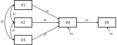
The population model under which we generated data was a path model on five variables that were originally evaluated by Cooke, Dahdah, Norman, & French (2016), and reanalyzed using MASEM by Cheung & Hong (2017). The meta-analytic path model was used to predict smoking behavior with the theory of planned behavior (Ajzen, 1991). Figure 1 shows the path model with the population parameter values that were used to generate the data. We evaluated the performance of MASEM-methods in conditions varying in the number of studies, the sample sizes within studies, the amount of missing correlation coefficients, and the amount of heterogeneity.

Figure 1. Population model with parameter values.

 

Number of studies

The example data set on which we base our population values included 33 studies. Reviews of applied MASEM studies indicated that a number of around 30 studies is typical in MASEM (Cheung & Chan, 2005; Furlow & Beretvas, 2005). Earlier simulation studies on MASEM evaluated conditions with 25, 50, and 100 studies (Furlow & Beretvas, 2010), 5, 10, 20, 50, 100, or 200 studies (Hafdahl, 2007), 10 and 30 studies (Furlow & Beretvas, 2005), and 5, 10, and 15 studies (Cheung & Chan, 2005). As fixed effects models are typically appropriate in groups of studies that all target a very specific population, we evaluate conditions with k = 10 and k = 30 studies. Furlow & Beretvas (2005) defined 10 studies as small and 30 studies as moderate.

Sample sizes within studies

The example data set had a median sample size of 170. Other simulation research where sample size was random within a study considered conditions with averages of 100, 300, and 1000 (Cheung, 2009), 50 and 100 (Furlow & Beretvas, 2010), and 5, 10, 20, 50, 100, and 200 (Hafdahl, 2007). Furlow & Beretvas (2005) used a fixed sample size of 100 for each study, and Cheung & Chan (2005) used fixed sample sizes of 50, 100, 200, 500, or 1000 for each study. We evaluated conditions where the average sample size within a study was 100 or 300, and we varied the specific sample sizes within each study using the positively skewed distribution as used in Hafdahl (2007). Specifically, the sample size n in each study k, equals n_k = (/2) [(χ²_k - 3)/] + , rounded to the nearest integer, where is 100 or 300 depending on the condition, and χ²_k is a random draw from a χ²(3)-distribution. This leads to expected distributions of n_k with a mean of , variance of and skewness of 1.63.

Missing variables

We did not vary the pattern and amount of missing variables. Instead, we fixed the pattern of missing variables to the one observed in the data set of Cooke. This means that all studies included the first three variables (V1–V3), 4 of the 30 studies missed V4, and 13 studies missed V5. In conditions with 10 studies, V4 and V5 were missing in, respectively, 1 and 4 of the studies.

Missing correlation coefficients

We evaluated conditions with correlation coefficients missing at random. There are no earlier simulation studies investigating the effect of missing correlations at the coefficient level, except for a very small one (Jak et al., 2013). Because missing correlation coefficients mostly occur when researchers do not report the correlation between two independent or two dependent variables, we selected the correlation between V1 and V2 and the correlation between V4 and V5 to be missing in part of the studies. We evaluated conditions where 0, 20, 50, or 70 % of these two correlation coefficients were missing. As V4 and V5 were already missing at the variable level in some studies, we removed correlation coefficients in 20, 50, or 70 % of the studies that included these variables. Note that even in the 0% missing coefficients level, there are missing correlations in studies due to missing variables.

Heterogeneity

To investigate the power to reject homogeneity at Stage 1, we generated data from two different populations. In population 1, the population correlation matrix was identical to Study 1. In population 2, all population correlations were 0.10 higher than in population 1. In the small heterogeneity condition, 20% of the studies were drawn from population 2 (and 80% from population 1), while in the large heterogeneity condition, 50% of the studies were drawn from population 2 (and 50% from population 1). This is similar to the conditions evaluated by Cheung & Chan (2005).

Misspecification at Stage 2

In order to evaluate the power to reject an incorrect model at Stage 2 (under homogeneity), we generated data from a model with a small (β = 0.10) effect of V3 on V5. At Stage 2, we fitted a path model without this direct effect. We obtained the expected power on the basis of the noncentrality parameter by fitting the path model without the direct effect to the population data (Saris & Satorra, 1993). The expected power in the conditions without missing correlation coefficients was 0.58 and 0.98 for conditions with k = 10 and n = 100 or n = 300, respectively, and 0.97 and 1.00 for conditions with k = 30 and n = 100 or n = 300, respectively.

Number of conditions and replications

Varying the factors number of studies (k = 10 or k = 30), average sample size within a study ( = 100 or = 300) and amount of missing correlations (zero, small, medium, or large) yielded 16 conditions in Study 1. In Study 2, we analyzed the same conditions with small and large heterogeneity at Stage 1, leading to 32 conditions. We generated 1000 meta-analytic data sets for each condition using the mvrnorm function in the MASS-package in R (R Core Team, 2016).

Study 1—Fitting the correct model

 

 

Expected differences between univariate approaches and multivariate approaches

Based on earlier simulation research (Cheung & Chan, 2005; Hafdahl, 2007), we expect similar performance across the methods when testing homogeneity at Stage 1. At Stage 2, it is expected that the univariate methods will reject the correct model too often, while the multivariate methods have false positive rates around the nominal alpha level.

The univariate approaches use the harmonic mean across correlation coefficients as the sample size at Stage 2. For the correlation between V4 and V5, the harmonic mean is larger than the actual sample size, while for the other correlations, the harmonic mean is smaller than the actual sample size. Therefore, we expect that with the univariate approaches, the standard errors for β₅₄ will be underestimated, while the standard errors of the other direct effects will be overestimated. We expect the differences to be the largest for β₅₄, because the largest missingness at the variable and correlation level is in the correlation between V4 and V5.

Expected differences between the two univariate approaches

The two univariate approaches that we evaluate only differ in whether the correlation matrix is analyzed correctly or not. UNI1 fits the model to the pooled correlation matrix as if it is a covariance matrix using maximum likelihood estimation. UNI2 analyzes the correlation matrix correctly using the diagonal constraint. We expect that UNI2 will perform better than UNI1, although both are expected to have biased standard errors due to missing data.

Expected differences between OC approach and OV approach

When there are no missing correlation coefficients, the OC and OV approach are equivalent. With increasing missing correlation coefficients, we expect that the standard errors in the OC approach will be smaller than those from the OV approach, and that the differences increase with increasing amount of missing correlations. Based on the model and conditions under which the population correlations were generated, we expect that the differences between the OC and OV approach will be largest for β₄₁ and β₄₂. The reason is that these two parameters will be directly affected if V1, V2, or V4 is deleted in the OV approach, while β₄₃ and β₅₄ are only affected if V4 is deleted. Moreover, there is already missingness on the variable level in V4 and V5, so the induced missingness (which is based on a percentage) is less in absolute value for these variables.

Expected differences between GLS and TSSEM

The GLS approach handles missing correlation coefficients at the coefficient-level, and is therefore expected to perform similarly to the OC-approach across different missing data conditions.

Results

All results from all conditions of both simulation studies are provided in the supplementary material. In the following section we will show a selection of the results graphically.

 

Nonconvergence

Nonconvergence only occurs for the TSSEM methods, as for the other methods the parameter estimates were not obtained iteratively. At Stage 1, convergence rates were not systematically different between the OC and OV approach or across different missing data conditions, and varied between 92% and 100% for k = 10, and between 97.2% and 100% for k = 30. We disregarded nonconverged solutions, and only fitted the Stage 2 model for the converged solutions. At Stage 2, all models converged in all conditions for all methods. The full results can be found in Table 2 in the supplementary material.

False positive rates

With 1000 data sets and a nominal α of 0.05, one would expect 95% of the results to lie within the interval [0.036–0.064].

Stage 1 (Testing homogeneity of correlations). False positive rates at Stage 1 are provided in Table 3 in the supplementary material. The false positive rates of the univariate methods were very small, and never exceeded 0.02. With the multivariate methods, the Stage 1 model was generally overrejected, especially when the within sample size was 100. With a within-study sample size of 300, the false positive rates were closer to 0.05 for all multivariate methods, but still higher than expected (ranging from 0.050 to 0.076). GLS showed somewhat better false positive rates than the OV and OC approach. False positive rates did not vary with missingness for any of the methods.

Stage 2 (Fitting the correct path model). A table with the false positive rates of the chi-square test when fitting the correct model at Stage 2 is provided in Table 4 in the supplementary material. As expected, the false positive rates of the univariate approaches are larger than the nominal alpha level, ranging from 0.111 to 0.169. The false positive rates of the multivariate approaches are within the limits of the prediction interval in all conditions, except for two cases in the k = 10 n = 100 condition where the false positive rate was 0.066 for both the OC and OV approach.

Bias in parameter estimates at Stage 2

Relative bias^{Figure 2, Figure 3, Figure 4} in the parameter estimates was very small (less than 2%) for all methods in all conditions, and is therefore not further discussed. The detailed results can be found in Tables 6–9 in the supplementary material.

Bias in standard errors at Stage 2

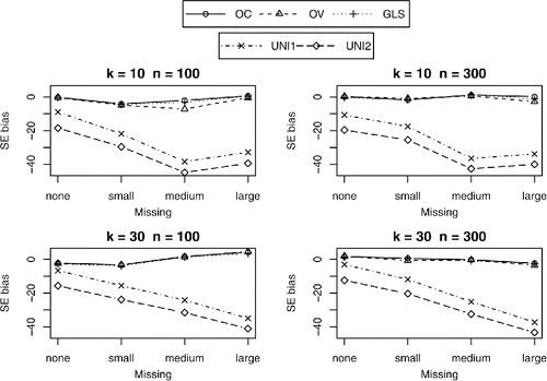
The standard errors of the multivariate methods were all relatively unbiased (with a maximum of 6% underestimation), and did not differ across the multivariate methods. As expected, the univariate methods showed increasingly biased standard errors with increasing amount of missing correlations. The standard errors were overestimated with univariate methods for those direct effects for which the harmonic mean was smaller than the actual sample size (for β₄₃, β₄₂, and β₄₁), and underestimated for direct effects where the harmonic mean was larger than the actual sample size (β₅₄). The tables and figures of the bias in SE’s for all regression coefficients can be found in the supplementary material (Tables 10–13 and Figures 10–13). Figures 2 and 3 show the percentages of bias in the standard errors for the parameters β₄₂ and β₅₄. With large amounts of missingness in conditions with k = 30 and n = 300, the univariate methods lead to standard errors that were up to 34% too large for β₄₂ and β₄₃, and up to 43% too small for β₅₄. As expected, UNI1 performed worse than UNI2.

Figure 2. Percentages of bias in standard error of β₄₂.

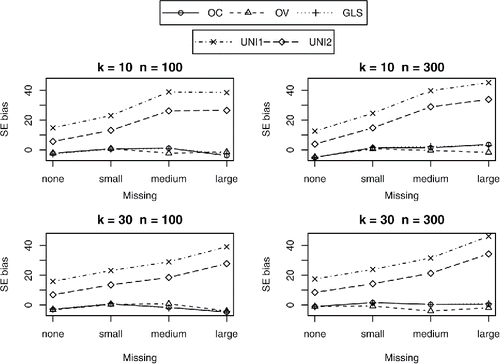
Figure 3. Percentages of bias in standard error of β₅₄.

Bias in standard errors at Stage 2 for alternative univariate methods

The results showed increasing bias in standard errors with increasing missingness for the univariate methods. As one of the reviewers suggested, this effect may partially be remedied by using the variances associated with the pooled correlation coefficients in a diagonal asymptotic covariance matrix in Stage 2. Moreover, we evaluated the univariate approach with sample size weighted coefficients (Schmidt & Hunter, 2015), and not with inverse variance weighted coefficients (Hedges & Olkin, 1985). In order to evaluate whether these alternative univariate approaches would perform better than UNI1 and UNI2 from the previous analyses, we ran additional simulations with inverse variance weighted methods. The results showed that the “naive” inverse variance weighted univariate method performed similarly to the UNI1 and UNI2 in the original simulation study. Using a diagonal asymptotic covariance matrix in the estimation of model parameters in Stage 2 lead to biased standard errors for both the sample size and inverse variance weighted methods, but as expected, the bias was not influenced by the amount of missing correlations. The best (but still not acceptable) performing univariate method was the inverse variance weighted method, with around 10 % relative bias in β₄₂ and −25 % relative bias in β₅₄ in all conditions. The full results can be found in Figures 14 and 15 in the supplementary material.

Size of standard errors at Stage 2

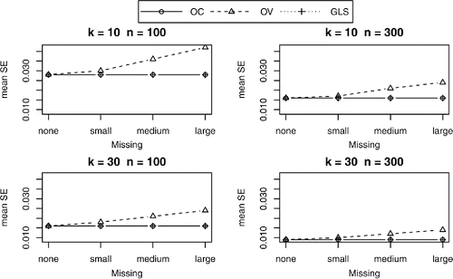
We will not evaluate the size of the standard errors of the univariate methods as they were found to be biased in all conditions. Looking at the size of the standard errors of β₄₂ for the multivariate approaches (Figure 4), we see that with missing correlations, the standard errors of the OC approach and GLS approach are equivalent, and slightly better (smaller) than those of the OV approach. With increasing missingness, the standard errors of OV increase rapidly, while with OC and GLS the size of the standard errors is quite stable. This is as expected because increases in the number of missing correlations imply the deletion of more data with the OV approach than with the OC or GLS approach. The same pattern is found for the other parameters (see Figures 16–19 in the supplementary material).

Figure 4. Mean standard error of β₄₂ for OC, OV, and GLS.

Study 2—Fitting a misspecified model

Expectations about statistical power

We expect that across methods, the power increases with the number of studies and sample size, and that the power decreases with increased missingness. The OC approach and GLS approach are expected to have higher power than the OV approach. The multivariate approaches are expected to have higher power than the univariate approaches. At Stage 1, more heterogeneity is expected to lead to larger power rates.

Results

 

Nonconvergence

Nonconvergence occurred more^{Table 1} often with heterogenous correlation matrices than under homogeneity (as evaluated in Study 1). At Stage 1, convergence rates were between 89.6% and 100% for small heterogeneity, and between 85.6% and 100% for large heterogeneity. Similar to Study 1, we disregarded nonconverged solutions. At Stage 2, all models converged in all conditions for all methods.

Power to reject heterogeneity at Stage 1

With small heterogeneity, empirical power rates were only acceptable (over 0.80) for the multivariate methods in the condition with 30 studies with an average sample size of 300 (see Figure 20 in the supplementary material). The univariate approaches showed insufficient power in all conditions with small heterogeneity. With large heterogeneity (see Figure 21 in the supplementary material), the multivariate methods had power rates over 0.80 in all conditions with average sample sizes of 300. The power rates of the OC method are consistently highest, followed by the OV approach and GLS. The univariate approaches showed acceptable power rates only in conditions with 30 studies and sample sizes of 300. Missingness does not seem to affect the power to reject homogeneity for any of the methods.

Power to reject a misspecified model at Stage 2

Figure 22 in the supplementary material shows the empirical power rates of rejecting a model with an omitted direct effect of size 0.10 of V3 on V5. The results in the conditions without missing correlations show the expected power levels for the multivariate methods. With 30 studies, all methods rejected the incorrect model in almost all cases. With 10 studies and an average within-study sample size of 300, all methods showed empirical power rates over 0.80, and only the OV approach shows a small decline in power with increasing missingness. In the conditions with 10 studies with an average sample size of 100, none of the methods had acceptable power rates. The univariate methods and the OV approach are strongly affected by missingness. The OC approach and GLS show a fairly stable power rate just below 0.60.

Discussion

Summary

Table 1 provides an overview of the main results from the simulation studies. Overall, both univariate methods performed poorly. Specifically, the standard errors were extremely biased at Stage 2 analysis. The bias could be either positive or negative depending on the patterns of the missing correlations. Moreover, the statistical power was lower than for the multivariate methods, and false positive rates at Stage 2 were inflated. The more correlation coefficients were missing, the poorer the performance of the univariate methods. From the multivariate methods, the OC approach performed best, although differences with GLS were minimal (the OC approach showed slightly better power rates at Stage 1). The OV approach showed similar performance as the OC approach and GLS in conditions with no missing correlation coefficients. However, with increasing missingness, the OV approach showed decreasing power levels and increasing standard errors at Stage 2. The results from the OC approach and GLS were quite stable across missing data conditions. Based on these results, we advise researchers to use multivariate approaches instead of univariate approaches for MASEM, and to apply the OC approach or GLS in the presence of many missing correlation coefficients.

Table 1. Summary of the results of the simulation study for the four MASEM methods under evaluation.

	Stage 1		Stage 2
Outcome Method	False positives	Power	False Positives	Power^*	Parameter bias	SE bias	SE efficiency
Univariate	Too small	Overall bad	Too large	Decreases with missingness	Unbiased	Biased	—
OV approach	Too large	Acceptable only with N = 300	Good	Decreases with missingness	Unbiased	Unbiased	SE increases with missingness
OC approach	Too large	Acceptable only with N = 300	Good	Stable	Unbiased	Unbiased	Stable (similar to GLS)
GLS	Too large	Acceptable only with N = 300	Good	Stable	Unbiased	Unbiased	Stable (similar to OC)

^*Power was acceptable for all methods in all conditions except for the k = 10, n = 100 conditions.

Shaded cells indicate that the method outperformed other methods for the criterion in the respective column.

Limitations and future research

This study is the first simulation study that evaluated the influence of missing correlation coefficients on the performance of MASEM methods under several realistic scenarios. However, we did not evaluate all possible conditions. For example, we only evaluated conditions where correlation coefficients were missing at random. We think this is a realistic situation, because not reporting correlation coefficients often happens because of the role of the variables in the analyses. For example, the correlation between two exogenous variables in a path model, or the correlation between two outcome variables in two separate regression analyses is often not reported. In such cases, the missingness of a coefficient is not related to the size of the coefficient, only to the role of the variables in the model. However, additional simulation research is needed to evaluate the performance of MASEM-methods in situations where missingness of a correlation coefficients is related to the size of the correlation. For example, if correlations are not reported because they were not strong enough to be significantly different from zero, applying MASEM will overestimate the strength of the relations between those variables.

This article focused on the evaluation of fixed-effects MASEM methods, because these are the models for which missing correlation coefficients are problematic. Models for random-effects MASEM generally account for missing correlation coefficients at the coefficient level, similar to fixed-effects GLS. As we found that GLS and the OC approach performed quite stable across missing data conditions, we expect their performance to be stable for random-effects models as well. Future simulation studies may verify these expectations.

Implementation

As the OC approach was found to perform best overall, it is important that this method is available to researchers. We wrote an R-function, Stage1.OC(), that can be used to apply Stage 1 of TSSEM using the OC approach. This function needs two arguments, a list with the correlation matrix for each study, and a vector with the sample sizes in the studies. In the supplementary material, we provide the link to download the function, and we provide an annotated example script using the OC approach on one of the generated data sets.

Conclusion

This study is the first to evaluate the performance of fixed-effects MASEM methods under different levels of missing correlation coefficients. We found that the univariate methods performed very poorly, while the multivariate methods performed well overall. Based on our results, we recommend using the OC approach or GLS when the amount of missing correlation coefficients is substantial, as these methods were most stable in conditions with increasing missing data. The univariate methods should not be used for MASEM.

Article information

Conflict of Interest Disclosures: Each author signed a form for disclosure of potential conflicts of interest. No authors reported any financial or other conflicts of interest in relation to the work described.

Ethical Principles: The authors affirm having followed professional ethical guidelines in preparing this work. These guidelines include obtaining informed consent from human participants, maintaining ethical treatment and respect for the rights of human or animal participants, and ensuring the privacy of participants and their data, such as ensuring that individual participants cannot be identified in reported results or from publicly available original or archival data.

Role of the Funders/Sponsors: None of the funders or sponsors of this research had any role in the design and conduct of the study; collection, management, analysis, and interpretation of data; preparation, review, or approval of the manuscript; or decision to submit the manuscript for publication.

Acknowledgments: The ideas and opinions expressed herein are those of the authors alone, and endorsement by the authors’ institutions or their funding agencies not intended and should not be inferred.

Additional information

Funding

Dr. Jak’s work was supported by Rubicon grant 446-14-003 from the Netherlands Organization for Scientific Research (NWO). Dr. Cheung’s work was supported by the Academic Research Fund Tier 1 (FY2013-FRC5-002) from the Ministry of Education, Singapore.

References

- Ajzen, I. (1991). The theory of planned behavior. Organizational Behavior and Human Decision Processes, 50(2), 179–211. doi: 10.1016/0749-5978(91)90020-t.
- Becker, B. J. (1992). Using results from replicated studies to estimate linear models. Journal of Educational Statistics, 17(4), 341–362. doi: 10.2307/1165128.
- Becker, B. J. (1995). Corrections to “using results from replicated studies to estimate linear models.” Journal of Educational and Behavioral Statistics, 20(1), 100–102. doi: 10.2307/1165390
- Becker, B. J. (2009). Model-based meta-analysis. In H. Cooper, L. V. Hedges, & J. C. Valentine (Eds.), The handbook of research synthesis and meta-analysis (2nd ed., pp. 377–395). New York, NY: Russell Sage Foundation.
- Bentler, P. M., & Lee, S.-Y. (1983). Covariance structures under polynomial constraints: Applications to correlation and alpha-type structural models. Journal of Educational and Behavioral Statistics, 8(3), 207–222. doi: 10.3102/10769986008003207
- Bergh, D. D., Aguinis, H., Heavey, C., Ketchen, D. J., Boyd, B. K., Su, P., … Joo, H. (2016). Using meta-analytic structural equation modeling to advance strategic management research: Guidelines and an empirical illustration via the strategic leadership-performance relationship. Strategic Management Journal, 37(3), 477–497. doi: 10.1002/smj.2338
- Card, N. A. (2015). Applied meta-analysisfor social science research. New York, NY: Guilford Publications.
- Cheung, M. W.-L. (2009). Comparison of methods for constructing confidence intervals of standardized indirect effects. Behavior Research Methods, 41(2), 425–438. doi: 10.3758/BRM.41.2.425
- Cheung, M. W.-L. (2015a). Meta-Analysis: A structural equation modeling approach. Chichester, West Sussex, U.K.: John Wiley & Sons.
- Cheung, M. W.-L. (2015b). metaSEM: An R package for meta-analysis usingstructural equation modeling. Frontiers in Psychology, 5. doi: 10.3389/fpsyg.2014.01521.
- Cheung, M. W.-L., & Chan, W. (2005). Meta-analytic structural equation modeling: A two-stage approach. Psychological Methods, 10(1), 40–64. doi: 10.1037/1082-989X.10.1.40
- Cheung, M. W.-L., & Chan, W. (2009). A two-stage approach to synthesizing covariance matrices in meta-analytic structural equation modeling. Structural Equation Modeling: A Multidisciplinary Journal, 16(1), 28–53. doi: 10.1080/10705510802561295
- Cheung, M. W.-L., & Hafdahl, A. R. (2016). Special issue on meta-analytic structural equation modeling: Introduction from the guest editors. Research Synthesis Methods, 7(2), 112–120. doi: 10.1002/jrsm.1212
- Cheung, M. W.-L., & Hong, R. (2017). Applications of meta-analytic structural equation modeling in health psychology: Examples, issues, and recommendations. Health Psychology Review, 11(3), 265–279. doi: 10.1080/17437199.2017.1343678
- Cheung, S. F. (2000). Examining solutions to two practical issues in meta-analysis: Dependent correlations and missing data in correlation matrices (Ph.D.). The Chinese University of Hong Kong, Hong Kong.
- Connelly, B. S., & Chang, L. (2016). A meta-analytic multitrait multirater separation of substance and style in social desirability scales. Journal of Personality, 84(3), 319–334. doi: 10.1111/jopy.12161
- Cooke, R., Dahdah, M., Norman, P., & French, D. P. (2016). How well does the theory of planned behaviour predict alcohol consumption? A systematic review and meta-analysis. Health Psychology Review, 10(2), 148–167. doi: 10.1080/17437199.2014.947547
- Cudeck, R. (1989). Analysis of correlation matrices using covariance structure models. Psychological Bulletin, 105(2), 317–327. doi: 10.1037/0033-2909.105.2.317
- Enders, C. K., & Bandalos, D. L. (2001). The relative performance of full information maximum likelihood estimation for missing data in structural equation models. Structural Equation Modeling, 8(3), 430–457. doi: 10.1207/s15328007sem08035
- Field, A. P. (2001). Meta-analysis of correlation coefficients: A Monte Carlo comparison of fixed-and random-effects methods. Psychological Methods, 6(2), 161–180. doi: 10.1037/1082-989x.6.2.161
- Furlow, C. F., & Beretvas, S. N. (2005). Meta-analytic methods of pooling correlation matrices for structural equation modeling under different patterns of missing data. Psychological Methods, 10(2), 227–254. doi: 10.1037/1082-989X.10.2.227
- Furlow, C. F., & Beretvas, S. N. (2010). An evaluation of multiple imputation for meta-analytic structural equation modeling. Journal of Modern AppliedStatistical Methods, 9(1), 129–143. doi: 10.22237/jmasm/1272687180
- Guan, M., & Vandekerckhove, J. (2016). A Bayesian approach to mitigation of publication bias. PsychonomicBulletin and Review 23, 74–86. doi: 10.3758/s13423-015-0868-6.
- Hafdahl, A. R. (2007). Combining correlation matrices: Simulation analysis of improved fixed-effects methods. Journal of Educational and Behavioral Statistics, 32(2), 180–205. doi: 10.3102/1076998606298041
- Hafdahl, A. R. (2008). Combining heterogeneous correlation matrices: Simulation analysis of fixed-effects methods. Journal of Educational and Behavioral Statistics, 33(4), 507–533. doi: 10.3102/1076998607309472
- Hafdahl, A. R., & Williams, M. A. (2009). Meta-analysis of correlations revisited: Attempted replication and extension of field’s (2001) simulation studies. Psychological Methods, 14, 24–42. doi: 10.1037/a0014697.
- Hedges, L., & Olkin, I. (1985). Statistical methods for meta-analysis. Orlando, FL: Academic Press.
- Hedges, L., & Vevea, J. (1998). Fixed- and random-effects models in meta-analysis. Psychological Methods, 3(4), 486–504.
- Hoogland, J. J., & Boomsma, A. (1998). Robustness studies in covariance structure modeling an overview and a meta-analysis. Sociological Methods & Research, 26(3), 329–367. doi: 10.1177/0049124198026003003
- Jak, S. (2015). Meta-analytic structural equation modelling. New York: Springer. doi: 10.1007/978-3-319-27174-3
- Jak, S., Oort, F. J., Roorda, D. L., & Koomen, H. M. (2013). Meta-analytic structural equation modelling with missing correlations. Netherlands Journal of Psychology, 67(4), 132–139.
- John, L. K., Loewenstein, G., & Prelec, D. (2012). Measuring the prevalence of questionable research practices with incentives for truth telling. Psychological Science, 23(5), 524–532. doi: 10.1037/e632032012-001
- Mesmer-Magnus, J. R., Asencio, R., Seely, P. W., & De Church, L. A. (2015). How organizational identity affects team functioning the identity instrumentality hypothesis. Journal ofManagement, Online first. doi: 10.1177/0149206315614370
- R Core Team. (2016). R: A language and environment for statistical computing. Retrieved from http://www.R-project.org.
- Rich, A., Brandes, K., Mullan, B., & Hagger, M. S. (2015). Theory of planned behavior and adherence in chronic illness: A meta-analysis. Journal of Behavioral Medicine, 38(4), 673–688. doi: 10.1007/s10865-015-9644-3
- Riley, R. D. (2009). Multivariate meta-analysis: The effect of ignoring within-study correlation. Journal of the Royal Statistical Society: Series A, 172(4), 789–811. doi: 10.1111/j.1467-985x.2008.00593.x
- Rosopa, P. J., & Kim, B. (2016). Robustness of statistical inferences using linear models with meta-analytic correlation matrices. Human ResourceManagement Review, 27(1), 216–236. doi: 10.1016/j.hrmr.2016.09.012.
- Rothstein, H. R., Sutton, A. J., & Borenstein, M. (2006). Publication bias in meta-analysis: Prevention, assessment and adjustments. New York: John Wiley & Sons.
- Saris, W., & Satorra, A. (1993). Power evaluations in structural equation models. In K. A. Bollen, & J. S. Long (Eds.), Testing structural equation models (pp. 181–204). Newbury Park, CA: Sage.
- Savalei, V., & Rhemtulla, M. (2012). On obtaining estimates of the fraction of missing information from full information maximum likelihood. Structural Equation Modeling: A Multidisciplinary Journal, 19(3), 477–494. doi: 10.1080/10705511.2012.687669
- Schmidt, F. L., & Hunter, J. E. (2015). Methods of meta-analysis: Correcting error and bias in research findings (3rd ed.). Thousand Oaks, CA: Sage Publications.
- Sheng, Z., Kong, W., Cortina, J. M., & Hou, S. (2016). Analyzing matrices of meta-analytic correlations: Current practices and recommendations. Research Synthesis Methods, 7(2), 187–208. doi: 10.1002/jrsm.1206
- Simonsohn, U., Nelson, L. D., & Simmons, J. P. (2014). P-curve and effect size: Correcting for publication bias using only significant results. Perspectives on Psychological Science, 9(6), 666–681. doi: 10.1177/1745691614553988
- Tang, R., & Cheung, M. W.-L. (2016). Testing IB theories with meta-analytic structural equation modeling: The TSSEM approach and the univariate-r approach. Review of InternationalBusiness and Strategy, 26(4), 472–492. doi: 10.1108/RIBS-04-2016-0022.
- Topa, G., & Moriano, J. A. (2010). Theory of planned behavior and smoking: Meta-analysis and SEM model. Substance Abuse and Rehabilitation, 1, 23–33. doi: 10.2147/sar.s15168.
- van Assen, M. A., van Aert, R., & Wicherts, J. M. (2016). Meta-analysis using effect size distributions of only statistically significant studies. Psychological Methods, 20(3), 293–309. doi: 10.1037/met0000025.
- Viswesvaran, C., & Ones, D. S. (1995). Theory testing: Combining psychometric meta-analysis and structural equations modeling. Personnel Psychology, 48(4), 865–885. doi: 10.1111/j.1744-6570.1995.tb01784.x.