Determining the nitrous oxide transfer velocity and emission factor of an agricultural drain

ABSTRACT

There have been few studies examining indirect nitrous oxide emissions associated with nitrogen (N) leaching from agricultural soils. For agricultural drainage water, equals the water’s concentration in excess of the atmospheric value multiplied by the transfer velocity . Using this equation, tracers and chamber methods, and were measured from an agricultural drain. Estimates of were made by measuring water speed and depth using the relationship developed by O’Connor and Dobbins [1958. Mechanisms of reaeration in natural streams. Transactions of the American Society of Civil Engineers. 123:641–684]. The measurements and estimates were not significantly different and averaged 5 m d⁻¹. Alternatively, for the method developed by the Intergovernmental Panel on Climate Change, equals the mass of N flowing in the water multiplied by an emission factor (EF). By additional measurements of the drain’s width, the water’s flow rate and nitrate () concentration, the estimated EF was 1.2 × 10⁻⁴kg kg⁻¹ .

KEYWORDS:

• Nitrous oxide
• transfer velocity
• indirect emission factor
• EF5
• IPCC

Introduction

In soils, nitrogen (N) containing compounds can be transformed to produce nitrous oxide , the third most important greenhouse gas (Davidson & Kanter 2014). In addition, is the primary source of nitrogen oxides which deplete stratospheric ozone (Ravishankara et al. 2009). Agriculture is considered the largest source of anthropogenic emissions (), estimated to account for about 70% of the total (Davidson & Kanter 2014).

In New Zealand, the direct from pastoral agriculture soils have been studied extensively (Kelliher et al. 2014). In contrast, there have been few studies of the indirect associated with N leaching from agricultural soils (Clough et al. 2006, 2007). For an agricultural drain, a diffusion equation can be written to show that the indirect will be equal to the water’s concentration, in excess of the atmospheric value, multiplied by the water to atmosphere transfer velocity for ().

The transfer velocity for oxygen (, also known as re-aeration and only differing from by the gas species diffusion coefficient) has been measured in five streams and two rivers in New Zealand (Wilcock 1984, 1988; Wilcock et al. 1995, 1999). In these studies, the results were consistently found to be strongly correlated with estimates determined by water speed and depth following O’Connor and Dobbins (1958). While the results exceeded the estimates by 40%, the estimates could simply be adjusted upwards.

Recently, in the United Kingdom, has been estimated for agricultural drains following O’Connor and Dobbins (1958) in a study by Hama-Aziz et al. (2017). These authors made no adjustments to their estimates and, to our knowledge, has not been measured in an agricultural drain. This leads to the first objective of our study which was to measure in an agricultural drain in New Zealand and compare the results with estimates determined by water speed and depth measurements following O’Connor and Dobbins (1958).

The Intergovernmental Panel on Climate Change (IPCC) represents the indirect from agricultural drainage water differently to the afore-mentioned diffusion equation with . For the method developed by the IPCC, equals the mass of N flowing in the water multiplied by an emission factor (EF; Reay et al. 2005). Since 1990, the IPCC method has been used to compile inventories for New Zealand’s agricultural soils (Ministry for the Environment 2016). For this reason, as our study’s second objective, additional measurements were made to estimate the indirect EF for an agricultural drain.

Methods

Experimental site

The experimental site was located 3 km East of Lincoln, New Zealand, along a 215-m-long reach of a spring-fed drain flowing South next to Rainey’s Road (43° 33.12′ S, 172° 32.693′ E). The surrounding land area of approximately 20 km² was mostly used for pastoral agriculture. The beginning of the experimental reach was located 1300 m from the spring. Beyond the reach, the drain emptied into the Halswell River.

Along the experimental reach (Figure 1), the drain’s gradient was 1.9 × 10⁻³m m⁻¹ (1.9 m fall per kilometre of reach) measured by a global positioning system. The water surface in the drain was located about 2 m below the level of the surrounding land. The drain’s cross-section was shaped like an upright, truncated letter V. The flat bottom of the drain averaged about 1 m wide and the top was about 4 m wide.

Figure 1. Photograph of the agricultural drain during experiment 2 on 12 August 2015, looking South, the direction the water was flowing.

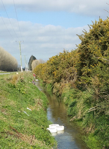
Along the experimental reach, a 20-m-tall hedge was located about 20 m to the West across Rainey’s Road. The slopes along the drain were covered with grasses and other herbaceous vegetation. The drain’s water was clear and mostly free of vegetation. Fine-textured sediment along the bottom was about 3–10 cm thick with gravel underneath.

For this study, the measurements were made during two experiments. Experiment 1 was performed in summer (20 January 2015) and experiment 2 in winter (12 August 2015). Both experiments were executed between 11 am and 1 pm, local standard time.

Measuring using a tracer method

The basis for the method will be described first, followed by the details. There were three tracers including propane (), bromide (Br) and Rhodamine dye. Known quantities of the tracers were mixed with water in a container. For an experiment, the contents were released into the drain at a constant, measured rate. After release, the drain’s water was sampled at a number of ‘downstream’ locations at times triggered by observation of the dye. The method was based on the drain water’s concentration decreasing at a rate determined by the transfer velocity from the water to the atmosphere (). The inert Br tracer was included to confirm the added water was present at the sampling points along the reach. To convert to , the estimated was multiplied by a ratio of the Schmidt numbers for and . The Schmidt number was used to characterise gas transfer under forced convection (turbulent) conditions as a dimensionless ratio of the momentum and mass diffusivities.

In the container, 80 L of water was mixed with 0.3 kg of potassium bromide for experiment 1 (2.5 g Br L⁻¹) and 1.0 kg for experiment 2 (8.4 g Br L⁻¹). For both experiments, the container was continuously purged with and the Rhodamine dye was added and mixed well before the contents were released into the drain at a rate of 1.7 × 10⁻⁶m³s⁻¹. Downstream of the release point, dye observation and water sampling locations were established at distances of 25, 50 and 150 m for experiment 1 and 25, 50, 150 and 200 m for experiment 2. Each sample was collected 10 cm below the water surface by slowly drawing 50 mL of water into a pre-flushed, gas-tight glass syringe fitted with a three-way stopcock (Cadence Science, Inc., Staunton, VA USA). The sample was then injected into a Helium-flushed, pre-evacuated 105 mL glass bottle fitted with a butyl rubber septum.

After returning to the laboratory, each bottle was thoroughly shaken, the headspace sampled and 10 mL of air was transferred to a pre-evacuated 6 mL vial. Each air sample’s concentration was measured using a gas chromatography system. There was a 2-m-long column containing Poropak Haysep B heated to 65°C, followed by a flame ionisation detector heated to 100°C (model 8610, SRI Instruments, Los Angeles, CA, USA). The detector was calibrated using five standards with concentrations of 20 (ambient air), 50, 100, 500 and 1000 μL L⁻¹.

Prior to the Br concentration measurement, the water samples were passed through a 0.45 μm nylon filter. An ion exchange chromatography system was used to measure the Br concentration (model Dionex ICS-2100, Thermo Fisher Scientific, Sunnyvale, CA, USA). The eluent was 200 mM sodium carbonate and the flow rate was 23 μL s⁻¹. For each sample, the injection volume was 25 μL. The chromatography system had a 50 mm long (4 mm inside diameter, id) guard column, a 250 mm long (4 mm id, IonPac AS9-SC) analytical column, a self-regenerating anion suppressor (Dionex AERS 500) and a conductivity detector. The detector was calibrated using a set of standards with concentrations of 0–2000 μg L⁻¹.

For data analysis, each concentration () was divided by that of the inert Br tracer (). Next, a logarithm (base e) was taken of each ratio (). Then, the slope of the relationship between () and time (between release and collection at the sampled locations) was determined by linear regression. This determined the mean rate of tracer loss from the drain’s water along the experimental reach.

To determine , the mean tracer loss rate was multiplied by the mean depth of water, , estimated using the following equation(1) where was the drain’s mean volumetric water flow rate (m³ s⁻¹), the mean water velocity (m s⁻¹) and the mean width (m). To determine , the Br tracer release rate into the drain was divided by the drain water’s mean Br concentration measured at water sampling locations which were 15, 40, 65 and 165 m downstream for experiment 1 and 15, 40, 65, 165 and 215 m downstream for experiment 2. To determine , the time taken for the Rhodamine dye to travel 40, 65 and 165 m was observed for each experiment, recorded and these data were statistically analysed by linear regression. For each experiment, a tape was used to measure at the water sampling locations.

The estimated was converted to by multiplying by where and were the Schmidt numbers for and , respectively. The power coefficient of −0.67 represented the drain having a flat water surface (i.e. no waves, Jähne et al. 1987). The Schmidt numbers were estimated by measuring the water temperature () throughout an experiment and inserting the mean value into the relationships reported by Wanninkhof (1992). These relationships were  = 2056–137  + 4.32 – 0.0544 and  = 1911–118  + 3.45  – 0.0413 .

To estimate the uncertainty of , standard errors (SEs) were estimated for the mean tracer loss rate and . For the mean tracer loss rate, the SE was determined by the regression analysis. For , a SE was first estimated for each term in Equation (1). For and , the SE was determined using the standard deviation from each sample of measurements which was then divided by a square root of the number of measurements. For , the SE was again determined by the regression analysis. For each term in Equation (1), the SE was divided by the mean, squared, summed and a square root of the sum was calculated. This was an estimate of the SE divided by the mean for . Then, for the mean trace loss rate and the SE was divided by the mean, squared, summed and a square root of the sum was calculated. This was an estimate of the SE divided by the mean for .

Measuring using a chamber method

The basis for this method was the following diffusion equation:(2) where c was concentration in the water () or the atmosphere () and was a dimensionless solubility coefficient following Henry’s Law. For this study, the units for were m d⁻¹, representing m³ N₂O m⁻²d⁻¹. Consequently, to calculate , the units of were μg m⁻²d⁻¹ and those for and were μg m⁻³.

This method was only used during experiment 2. As described earlier, was released throughout experiment 2 at a constant, measured rate into the drain at the beginning of the experimental reach. A chamber method was used to measure the emissions () and the chamber design was described earlier (Clough et al. 2006). Briefly, the polypropylene chamber was 117 mm tall, 107 mm wide on average, and the top was fitted with a butyl rubber septum for air sampling. There was an 85 mm wide annulus of polystyrene, so the chamber floated, but by offsetting it from the annulus the chamber projected 15 mm into the water.

There were six chambers, three were located 25 m downstream from the C₃H₈ release point and the other three were 150 m downstream (Figure 1). After each chamber was placed on the water in the middle of the drain, four air samples were collected using a syringe and the septum at 15 minute intervals. Two ambient air samples were also collected. For each sample, 10 mL was then injected into a Helium-flushed, pre-evacuated 6 mL glass bottle fitted with a butyl rubber septum. The sample’s concentration was measured using the gas chromatography system described earlier.

For data analysis, linear regression was used to estimate the rate of change in headspace concentration. To determine , the rate was multiplied by two ratios, the chamber volume divided by the surface area and the atmospheric pressure divided by a product of the universal gas constant and the temperature. To determine , the mean concentrations in the water and atmosphere from the ambient samples were combined with . Then, following Equation (2), was estimated by a ratio of the estimated values for and . The estimated was then converted to using the corresponding Schmidt numbers as described earlier. To estimate the uncertainty of , the SE was determined by the standard deviation of the six measurements divided by the square root of six.

Estimating using water speed and depth measurements

To estimate , we used a relationship developed by O’Connor and Dobbins (1958)(3) where D_N20inwater was the N₂O (mass) diffusivity in water. To determine for each experiment, the mean water temperature was inserted in an equation reported by Tamimi et al. (1994). The determination of and have been described earlier.

To determine the uncertainty of the estimated , SEs were estimated for each component of Equation (3). For , it was assumed there had been no uncertainty. For and , determination of the SEs was described earlier. For these two terms, the SE was divided by the mean, squared, summed and a square root of the sum was calculated. This was an estimate of the SE divided by the mean for .

Estimating an indirect EF

As stated, for the method developed by the IPCC, equals the mass of N flowing in the water multiplied by an indirect EF. On this basis, an EF can be estimated by determining and the mass of N flowing in the water. This was done for experiment 2 by making additional measurements on the collected water samples.

The basis for determining was Equation (2). To estimate , we used Equation (3) and the inputs were determined as described above. To determine , the concentrations of the water and (ambient) air samples were measured using the gas chromatography system, an electron capture detector operated at 310°C and calibrated using five standards with concentrations of 0.00 (di-nitrogen gas), 0.20, 0.32 (ambient air), 0.50 and 1.00 μL L⁻¹.

The mass of N flowing in the drain equals the flow rate multiplied by the N concentration. The flow rate was determined as described above. To determine the N concentration, additional measurements were made on the water samples. Flow injection methods were used to measure the sample’s nitrate () and ammonium () concentrations (model FIAstar™ 5000 analyser, FOSS, Hilleroed, DK). For , following Foss method AN 5232, the sample was mixed with an chloride buffer (pH 8.5) and reduced to nitrite () using a cadmium coil. By adding acidic sulphanilamide and a Greiss reagent, a purple azo compound formed. The radiation absorbance was then measured using a calibrated spectrophotometer at a wavelength of 540 nm. Re-analysis without the cadmium coil determined the initial concentration, and hence by subtraction, the concentration was determined. The detection limit was 1 × 10⁻⁷kg L⁻¹. Foss method AN 5220 was used to determine the concentration, but all of the results were less than the detection limit of 5 × 10⁻⁷kg L⁻¹.

Finally, the units for EF were kg kg⁻¹ . The units for the mass of N flowing in the water were kg d⁻¹. Consequently, the units for were converted from kg m⁻²d⁻¹ to kg d⁻¹. This was done by estimating the water area associated with one day of emissions from the mean flow rate (m³d⁻¹) multiplied by the drain’s mean width. The uncertainty of the EF estimate was determined as described above.

Results

For experiment 1, using the tracer method, the slope of the relationship between Ln([]/[Br]) and time was 50 ± 5 μL L⁻¹d⁻¹ (± SE). To calculate , this result was multiplied by determined using Equation (1). The components of Equation (3) included which was 0.057 ± 0.0004 m³s⁻¹, was 0.294 ± 0.002 m s⁻¹ and was 1.45 ± 0.025 m. Consequently, was 0.134 ± 0.003 m and was 6.7 ± 0.6 m d⁻¹. The mean water temperature was 15.3°C, so the quantity was 0.99. Multiplying by 0.99 yielded which was 6.6 ± 0.6 m d⁻¹ (Table 1).

Table 1. The nitrous oxide () transfer velocity from an agricultural drain to the atmosphere (, mean ± SE) determined by experiments 1 (20 January 2015) and 2 (12 August 2015).

Date	measured by a tracer method	measured by a chamber method	estimated following O’Connor and Dobbins (1958)
	m d^−1	m d^−1	m d^−1
20 January 2015	6.6 ± 0.6	No data	5.1 ± 1.0
12 August 2015	3.8 ± 0.6	4.8 ± 0.4	3.9 ± 0.6

Notes: As described in the text, the measurements used tracer and chamber methods. The estimates were based on hydraulic measurements and a relationship reported by O’Connor and Dobbins (1958).

To estimate for experiment 1 using the O’Connor and Dobbins (1958) relationship, the mean water temperature determined to be 1.38 × 10⁻⁴m²d⁻¹. The corresponding estimate of given above was converted to 25,402 ± 170 m d⁻¹ and was 0.134 ± 0.003 m as stated. After inserting these three values into Equation (3), the estimated was 5.1 ± 1.0 m d⁻¹.

For experiment 2, the slope of the relationship between Ln([]/[Br]) and time was 18 ± 1 μL L⁻¹d⁻¹. The estimated was 0.106 ± 0.001 m³s⁻¹, was 0.292 ± 0.003 m s⁻¹, was 1.72 ± 0.26 m and was 0.211 ± 0.032 m. As before, by a product of the slope and , was 3.8 ± 0.6 m d⁻¹. The mean water temperature was 11.9°C, the quantity ( was 0.99 and was 3.8 ± 0.6 m d⁻¹.

For experiment 2, the estimated was 1.30 × 10⁻⁴m²d⁻¹. The corresponding estimate of given above was converted to 25,200 ± 259 m d⁻¹ and was 0.211 ± 0.032 m as stated. After inserting these three values into Equation (3), the estimated was 3.9 ± 0.6 m d⁻¹.

Using the chamber method, on average during experiment 2, linear rates of change in the headspace concentration accounted for 97 ± 4% of the variability. Consequently, during the hour when the headspace air samples had been collected, there was no evidence that accumulation of had changed the water to atmosphere gradient represented by ) in Equation (2). By this method, the mean for experiment 2 was 4.8 ± 0.4 m d⁻¹.

For experiment 2, the drain water’s mean concentration was 2.78 ± 0.003 × 10⁻⁶kg L⁻¹. Multiplying this value by and converting the units, the mass of N flowing in the water was 25.5 ± 0.2 kg d⁻¹. The converted value of was 3.1 ± 0.7 × 10⁻³kg d⁻¹. Thus, the estimated EF was 1.2 ± 0.3 × 10⁻⁴kg kg⁻¹ .

Discussion

From experiment 2, the mean measured using the tracer method was nearly identical to the estimate following O’Connor and Dobbins (1958). The mean measured using the tracer method was 1.0 m d⁻¹ (21%) less than that measured using the chamber method. However, this difference was not statistically significant according to an unpaired T test (P = 0.20). For experiment 1, while the mean measured using the tracer method was 29% greater than the estimate, the difference was not statistically significant. Consequently, there was insufficient evidence from these experiments to reject our hypothesis.

For re-aeration, the O’Connor and Dobbins (1958) equation represented the renewal of oxygen to the (water) surface (Danckwerts 1951) by accounting for and . As indicated, the water to atmosphere transfer velocity called represented an N₂O escape coefficient for determining by diffusion according to ) using Equation (2). For experiments 1 and 2, as stated, the two values of were nearly identical. However, was 0.078 m or 58% larger in winter for experiment 2 and estimated following O’Connor and Dobbins (1958) was 1.2 m d⁻¹ or 24% smaller.

The variables and have also been combined in a ratio called the Froude number (Fr) which represents the inertial force () divided by the gravity force ( where g was the acceleration due to gravity, 9.8 m s⁻²). For experiments 1 and 2, Fr was 0.26 and 0.20, respectively. Such values can be interpreted to indicate that water flow was tranquil and the surface smooth as observed in the agricultural drain during our experiments.

For the IPCC, the EF for groundwater and agricultural drains has been called EF5-g (Reay et al. 2005). As stated, by dividing the estimated by the corresponding mass of N flowing in the water, the estimated EF5-g was 1.2 ± 0.3 × 10⁻⁴kg kg⁻¹ . To our knowledge, Reay et al. (2005) has been the only other study to have estimated EF5-g for agricultural drains. Their study was done in the United Kingdom and an alternative method was used to estimate EF5-g; namely, by sampling the water, measuring the dissolved () and the concentrations and determining the relationship by linear regression analysis. For Reay et al. (2005), the estimated mean EF5-g was 2.0 × 10⁻³kg kg⁻¹ . For this study, EF5-g can also be estimated using the alternative method and the measurements made during experiment 2. The mean was 4.16 ± 0.23 × 10⁻⁹kg L⁻¹. As stated, the corresponding mean concentration was 2.78 ± 0.003 × 10⁻⁶kg L⁻¹. Thus, by dividing the mean by the mean concentration, the alternatively estimated EF5-g was 1.5 ± 0.1 × 10⁻⁴kg kg⁻¹ . Consequently, we found two methods of determining EF5-g yielded similar estimates, but they were only 7–8% of the value reported by Reay et al. (2005).

In conclusion, measurements of an agricultural drain’s water to atmosphere transfer velocity for were not significantly different to estimates following O’Connor and Dobbins (1958). Consequently, the transfer velocity could be confidently estimated from measurements of water velocity, depth and temperature which determined the diffusivity. For the experiments conducted in summer and winter, the estimated transfer velocity averaged 5 m d⁻¹. Alternatively, two versions of the IPCC method to estimate the indirect EF (EF5-g) yielded similar results which averaged 1.4 ± 0.1 × 10⁻⁴kg kg⁻¹ . Using New Zealand’s first estimates of the transfer velocity or EF5-g, a previously unknown component of the indirect emissions associated with N leaching from agricultural soils can be determined.

Acknowledgements

We thank Rebecca D’Souza, Jen Owens, Shiv Prasad Pokhrel and Teresa Symon for helping us to collect the samples and measure the bromide, nitrate, nitrous oxide and propane concentrations. We also thank Brent Conlan for processing an image file to produce Figure 1.

Disclosure statement

No potential conflict of interest was reported by the authors.

References

- Clough TJ, Bertram JE, Sherlock RR, Leonard RL, Nowicki BL. 2006. Comparison of measured and EF5r-derived N2O fluxes from a spring-fed river. Global Change Biology. 12:352–363. doi: 10.1111/j.1365-2486.2005.01089.x
- Clough TJ, Buckthought LE, Kelliher FM, Sherlock RR. 2007. Diurnal fluctuations of dissolved nitrous oxide (N2O) concentrations and estimates of N2O emissions from a spring-fed river: implications for IPCC methodology. Global Change Biology. 13:1016–1027. doi: 10.1111/j.1365-2486.2007.01337.x
- Danckwerts PV. 1951. Significance of liquid-film coefficients in gas absorption. Industrial and Engineering Chemistry. 43:1460–1467. doi: 10.1021/ie50498a055
- Davidson EA, Kanter D. 2014. Inventories and scenarios of nitrous oxide emissions. Environmental Research Letters. 9:105012. doi: 10.1088/1748-9326/9/10/105012
- Hama-Aziz ZQ, Hiscock KM, Cooper RJ. 2017. Indirect nitrous oxide emission factors for agricultural field drains and headwater streams. Environmental Science and Technology. doi:10.1021/acs.est.6b05094.
- Jähne B, Münnich KO, Bösinger R, Dutzi A, Huber W, Libner P. 1987. On the parameters influencing air-water gas exchange. Journal of Geophysical Research. 92:1937–1949. doi: 10.1029/JC092iC02p01937
- Kelliher FM, Cox N, van der Weerden TJ, de Klein CAM, Luo J, Cameron KC, Di HJ, Giltrap D, Rys G. 2014. Statistical analysis of nitrous oxide emission factors from pastoral agriculture field trials conducted in New Zealand. Environmental Pollution. 186:63–66. doi: 10.1016/j.envpol.2013.11.025
- Ministry for the Environment. 2016. New Zealand’s greenhouse gas inventory 1990–2014. Available from: http://www.mfe.govt.nz/publications/climate-change/new-zealands-greenhouse-gas-inventory-1990-2014.
- O’Connor DJ, Dobbins E. 1958. Mechanisms of reaeration in natural streams. Transactions of the American Society of Civil Engineers. 123:641–684.
- Ravishankara AR, Daniels JS, Portmann RW. 2009. Nitrous oxide (N2O): the dominant ozone-depleting substance emitted in the 21st century. Science. 326:123–125. doi: 10.1126/science.1176985
- Reay DS, Smith KA, Edwards AC, Hiscock KM, Dong LF, Nedwell DB. 2005. Indirect nitrous oxide emissions: revised emission factors. Environmental Sciences. 2:153–158. doi: 10.1080/15693430500415525
- Tamimi A, Rinker EB, Sandall OC. 1994. Diffusion coefficients for hydrogen sulfide, carbon dioxide, and nitrous oxide in water over the temperature range 293–368 K. Journal of Chemical and Engineering Data. 39:330–332. doi: 10.1021/je00014a031
- Wanninkhof R. 1992. Relationship between wind speed and gas exchange over the ocean. Journal of Geophysical Research. 97:7373–7382. doi: 10.1029/92JC00188
- Wilcock RJ. 1984. Methyl chloride as a gas-tracer for measuring stream reaeration coefficients – II: stream studies. Water Research. 18:53–57. doi: 10.1016/0043-1354(84)90047-2
- Wilcock RJ. 1988. Study of river reaeration at different flow rates. Journal of Environmental Engineering. 114:91–105. doi: 10.1061/(ASCE)0733-9372(1988)114:1(91)
- Wilcock RJ, Champion PD, Nagels JW, Croker GF. 1999. The influence of aquatic macrophytes on the hydraulic and physico-chemical properties of a New Zealand lowland stream. Hydrobiologia. 416:203–214. doi: 10.1023/A:1003837231848
- Wilcock RJ, McBride GB, Nagels JW, Northcott GL. 1995. Water quality in a polluted lowland stream with chronically depressed dissolved oxygen: causes and effects. New Zealand Journal of Marine and Freshwater Research. 29:277–288. doi: 10.1080/00288330.1995.9516661