Variability of recurrence interval and single-event slip for surface-rupturing earthquakes in New Zealand

ABSTRACT

Recurrence interval (RI) and single-event slip (SES) for large-magnitude earthquakes that ruptured the ground surface (M_w > 6–7.2) can vary by more than an order of magnitude on individual faults. Frequency histograms, probability density functions (PDFs) and coefficient of variation (C_v, standard deviation/arithmetic mean) values for geological and simulated earthquakes on over 100 New Zealand active faults have been used to quantify RI and SES variability. Histograms of RI and SES for geological paleoearthquakes were constructed using a Monte Carlo method which accounts for the observations and their uncertainties. For the best of the geological PDFs (i.e. ≥7 surface-rupturing events) and earthquake simulations, RI are positively skewed with long recurrence tails (c. three times the mean) which are approximately described by log-normal and Weibull distributions. The geometric mean and coefficient of variation (C_vln) calculated for these log-normal distributions may be up to a factor of two lower and higher, respectively, than those determined assuming a normal distribution. By contrast, SES for geological and simulated earthquakes is often approximately normally distributed and appears to be less variable than RI (RI C_v 0.6 ± 0.2 geological and 0.6 ± 0.3 simulations; SES C_v 0.4 ± 0.2 geological). Variations in earthquake RI and to a lesser extent SES produce order-of-magnitude changes in slip rate over time intervals up to five times the arithmetic mean RI. Quantifying variability of RI, SES and slip rates is important when producing estimates of seismic hazard for surface-rupturing earthquakes, and could be estimated for active faults with poorly constrained paleoearthquake histories using the PDFs presented here.

KEYWORDS:

• Minimum magnitude of completeness
• paleoearthquakes
• recurrence interval
• simulated seismicity
• single-event slip

Introduction

Large-magnitude earthquakes pose major hazards in plate boundary regions, such as New Zealand where seismicity is driven by relative motion between the Pacific and Australian tectonic plates (Beavan et al. 2002). Forecasts of when and where these earthquakes will occur in the future carry significant uncertainty, in part because recurrence intervals (RI; i.e. inter-event times) and single-event slip (SES) can vary on individual faults over timescales of 10²–10⁵ years (e.g. Wallace 1987; Marco et al. 1996; McCalpin & Nishenko 1996; Xu & Deng 1996; Dawson et al. 2003; Friedrich et al. 2003; Palumbo et al. 2004; Weldon et al. 2004; Mouslopoulou et al. 2009a). Variable geological recurrence interval (RI) and single-event slip (SES) data are consistent with numerical earthquake simulations for fault systems (Robinson 2004; Robinson et al. 2009a, 2009b, 2011; Tullis et al. 2012a, 2012b). The size of this variability, what geological processes produce it and how it should be incorporated into hazard models are key unresolved questions. Quantifying the variability of RI and SES for large-magnitude surface-rupturing earthquakes is an important step for understanding earthquake processes and improving seismic hazard models.

In this paper we utilise a large quantity of published and unpublished geological data on the timing and slip of paleoearthquakes amassed in New Zealand, particularly over the last 30 years (Figure 1, Table 1, Dataset S1; Stirling et al. 2012; Litchfield et al. 2014). Paleoearthquake data are primarily for strike-slip and normal faults which, in part, reflect the fact that these fault types form the best-preserved fault traces. Geological data are complemented by moderate–large-magnitude earthquakes (M_w >4) generated by numerical earthquake simulations for active fault systems in the Wellington, Marlborough and Bay of Plenty regions of New Zealand (Figure 1, including 12 of the faults in Table 1) (Robinson 2004; Robinson et al. 2009a, 2009b, 2011). Synthetic earthquakes help fill information gaps in the geological data which may arise due to measurement uncertainty and to the brevity of the geological record (<10 surface-rupturing earthquakes are recorded on each fault analysed; Table 1). Together geological and synthetic earthquakes provide a large dataset for estimating the variability of RI and SES. Here, presentation of the data (i.e. sources and sampling biases) and methods of analysis are augmented by discussion of the geological and simulated surface-rupturing earthquake RI and SES for a range of fault types, slip rates and dimensions. These datasets are used to develop frequency histograms, probability density functions (PDFs) and coefficient of variation (C_v, normal distributions; C_vln, log-normal distributions) for RI and SES. The present study focuses on quantifying the variability of RI and SES and includes some discussion of how it could be accounted for in probabilistic seismic hazard analysis.

Figure 1. Active fault map of New Zealand showing the locations of faults (thick black lines). Fault numbers correspond to those given in the left-hand column of Table 1. Fault locations from the GNS Science active faults database (GNS open access, August 2012). Boxes show regions of simulated seismicity models (see text for further discussion of the models).

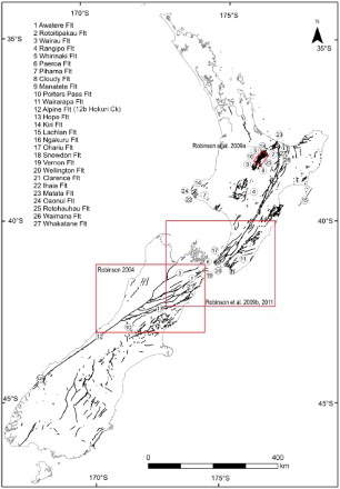
Table 1. Summary of faults and paleoearthquake information from geological datasets in this study. Timing of events and recurrence intervals have been rounded to the nearest 10 years. SES (and uncertainty) has been rounded to the nearest 10 cm. See Dataset S1 for paleoearthquake data and Figure 1 for fault locations. Refer to source publications for detailed paleoearthquake information.

	Fault	Fault type‡	Slip rate†		No. EQs	Recurrence (yr)		Single event slip (m)		Sim. EQs	Oldest event		Last event		Data sources
			(mm a^–1)	Error (2σ)		Mean	Std dev	Mean	Std dev	Y/N	Years before 2010	Error (2σ)	Years before 2010	Error (2σ)
1	Eastern Awatere	SS	6	2	9	930	540	5.2*	0.2	Y	8530	140	162	0	Benson et al. (2001), Mason et al. (2006)
2	Rotoitipakau	N	1.7	0.1	9	1315	1130	–	–	N	10560	1000	23	0	Berryman et al. (1998)
3	Wairau	SS	3.2	0.5	9	2260	1340	7.7	2.4	Y	17960	2300	2000	100	Zacheriasen et al. (2006), Barnes and Pondard (2010),Van Dissen & Nicol unpub. data 2012
4	Rangipo	N	0.23	0.03	8	1890	1570	0.5*	0.4	N	12110	250	1010	250	Villamor et al. (2007)
5	Whirinaki	N	0.7	0.3	8	3360	2050	0.9	0.4	Y	24060	3000	560	50	Canora-Catalán et al. (2008)
6	Paeroa	N	1.6	0.2	7	2620	1990	1.8	1.0	Y	16200	800	460	140	Berryman et al. (2008)
7	Pihama	N	0.1	0.05	7	10660	8180	0.9	0.4	N	67060	12500	3060	3000	Townsend et al. (2010), Mouslopoulou et al. (2012), Nicol et al. unpub. data 2011
8	Cloudy	SS?	2.5	1.5	6	3000	2120	2.9	1.8	N	16200	3700	1800	300	Pondard & Barnes (2010)
9	Mangatete	N	0.5	0.1	6	4640	1480	1	0.4	N	24210	2350	1010	750	Nicol et al. (2007), Nicol et al. unpub. data 2011
10	Eastern Porter's Pass	SS	3.6	0.5	6	1630	960	6.3	1.2	N	8760	300	610	50	Howard et al. (2005)
11	Southern Wairarapa	SS/R	11	3	6	1330	360	16.9*	3.4	Y	6825	155	155	0	Rodgers & Little (2006), Little et al. (2009), Van Dissen et al. (2013)
12	Alpine (central)	SS	27	4	5	149	47	8.5*	0.5	Y	780	50	184	25	Wells et al. (1999), Wells & Goff (2007), Yetton & Wells (2010)
12b	Southern Alpine (Hokuri Creek)§	SS	27	3	24	329	68	7.5*	1	N	7923	61	293	0	Berryman et al. (2012), Biasi et al. (2015)
13	Hope (Hope Segment)	SS	14	3	5	130	30	2*	0.6	Y	630	34	122	0	Cowan (1990), Cowan & McGlone (1991)
14	Kiri	N	1.4	0.3	5	910	710	–	–	N	4560	1500	990	770	Townsend et al. (2010), Mouslopoulou et al. (2012), Nicol et al. unpub. data 2011
15	Lachlan	R	4.5	1.5	5	1180	620	–	–	N	5343	75	610	100	Berryman (1993), Barnes et al. (2002)
16	Ngakuru	N	0.5	0.1	5	8540	5380	1.4	0.6	Y	26320	920	690	300	Nicol et al. unpub. data 2011
17	Ohariu	SS	1.5	0.5	5	1180	460	–	–	Y	4900	500	205	55	Heron et al. (1998), Litchfield et al. (2006), Litchfield et al. (2010), Van Dissen et al. (2013)
18	Snowdon	N	0.2	0.1	5	4760	2710	0.5	0.2	N	20060	2500	1010	750	Nicol et al. (2007), Nicol et al. unpub. data 2011
19	Vernon	SS	3	2	5	3140	1890	1.2	0.8	N	15300	3500	3200	700	Pondard & Barnes (2010), Bartholomew et al. (2014)
20	Wellington (Hutt Valley)	SS	6.1	2	5	1910	1440	5.0	1.5	Y	7895	545	270	545	Little et al. (2010), Langridge et al. (2011), Rhoades et al. (2011)
21	Eastern Clarence	SS	4	1	4	1590	920	7.0*	2	Y	6600	400	1820	160	Van Dissen & Nicol (2009)
22	Ihaia	N	0.35	0.15	4	1820	680	–	–	N	5860	500	410	200	Mouslopoulou et al. unpub. data 2011, Mouslopoulou et al. (2012)
23	Matata	N	4.1	1.5	4	790	490	–	–	N	2560	800	270	50	Ota et al. (1988), Begg & Mouslopoulou (2010)
24	Oaonui	N	0.11	0.04	4	7620	2770	0.5	0.1	N	23800	1200	990	720	Townsend et al. (2010)
25	Rotohauhau	N	0.6	0.1	4	5100	4870	0.8	0.2	Y	16360	900	1010	750	Nicol et al. (2007), Nicol et al. unpub. data 2011
26	Waimana (north)	SS/N	1.2	0.7	4	2910	940	–	–	N	11060	1500	2310	450	Mouslopoulou (2006), Mouslopoulou et al. (2009b)
27	Whakatane (north)	SS/N	2	1	4	2450	1970	–	–	N	8800	700	1460	700	Mouslopoulou (2006), Mouslopoulou et al. (2009b)

*Mean single-event slip calculated for two or three events only.

†Slip rates calculated for approximately the duration of the paleoearthquake record.

‡Slip types: SS, strike slip; N, normal; R, reverse; SS/R, mainly strike slip with some reverse; SS/N, mainly strike slip with some normal.

§Monte Carlo analysis of RI for the southern Alpine Fault not undertaken here; a more robust statistical analysis has been published by Biasi et al. (2015).

Geological paleoearthquake data

Active fault traces in New Zealand were mainly produced by surface-rupturing earthquakes over the last 30 ka (e.g. Figure 1; Stirling et al. 2012; Litchfield et al. 2014; this study). Over the last 30 years, analysis of fault trench logs and displacement of dated landforms has generated a large body of data on the paleoearthquake histories of these active faults (e.g. Table 1). These datasets provide evidence of progressive displacement and deformation of dated near-surface stratigraphy or geomorphic surfaces which enable the timing and/or slip during prehistoric earthquakes to be estimated (for discussion of methods see McCalpin 2009). These data mainly provide information for <10 surface-rupturing earthquakes on individual faults in New Zealand over time intervals of <30 ka (Table 1). For the purposes of this study, we utilise published and unpublished information for faults on which four or more past earthquakes have been recorded; the lower cut-off of four events is arbitrary and was selected to balance the requirements for statistically useful results and a large dataset of faults (detailed analysis of RI was only conducted on active faults with seven or more recorded events). Table 1 lists 27 faults that satisfy this criterion (≥4 events) and for which their paleoearthquake histories have been analysed. Paleoearthquake histories from the literature have been assumed correct except where these papers are augmented by later work (either published or unpublished); in this case we have generated earthquake histories that are consistent with all of the available data. In some instances, we have elected not to accept the proposed timing of prehistoric earthquakes because the inferences previously presented have been superseded by new data (see Table 1 and Dataset S1 for all references). The number of prehistoric events for which RI was estimated in this study varies between faults from 4 to 10 (c. 70% ≤6; statistics of RI for 24 events on the southern Alpine Fault have been studied in detail by Berryman et al. 2012; Biasi et al. 2015 and are not examined here), while the record of SES is generally less complete. In about two-thirds of cases, estimates of the SES are only available for the last one or two surface-rupturing events.

As with most paleoearthquake studies globally, geological estimates of the timing and slip of events in New Zealand include some measurement uncertainty (e.g. Stein & Newman 2004; McCalpin 2009; Nicol et al. 2009). Measurement uncertainties on the average SES and earthquake timing for paleoearthquakes in this study are generally ≤ c. ± 40% (Dataset S1). Uncertainties increase with the age of the earthquake and with the number of subsequent events. They also increase with a decrease in the number of observations constraining the timing and slip during a particular earthquake at a given site. Uncertainties for paleoearthquakes are adopted from source documentation or, where there are multiple documents, revised in accordance with the highest-quality data available.

Sampling artefacts

In addition to measurement uncertainties, RI and SES could be influenced by a number of sampling artefacts which, like the measurement uncertainties, impact all studies of paleoearthquakes (e.g. Stein & Newman 2004; McCalpin 2009; Nicol et al. 2009). These artefacts partly arise because paleoseismic data only sample the upper tip line of fault surfaces that in some cases extend to depths of tens of kilometres. Many paleoearthquake observations are point samples and can affect measurements of earthquake parameters when (1) each event does not rupture the entire length of a fault trace; (2) SES varies along a trace for an individual earthquake (e.g. Figure 2); and (3) changes in slip distributions along fault traces occur between earthquakes (e.g. Hemphill-Haley & Weldon 1999; Biasi & Weldon 2006; Wesnousky 2008; Little et al. 2010; Nicol et al. 2010; Hecker et al. 2013). Point-sample measurement of earthquake parameters will most often depart from mean or maximum values on long faults and/or approaching fault tips. Along the Alpine Fault in New Zealand, for example, which is at least 500 km in length, only two of five events appear to have ruptured the southern end of the fault since c. AD 900 (Howarth et al. 2014). The mean RI of 329 ± 68 years for the last c. 8000 years at a point towards the southern end of the fault trace (Berryman et al. 2012; Biasi et al. 2015) may therefore be greater than the mean RI for the entire fault trace (Biasi et al. 2015). If the earthquake timing and rupture dimensions since c. AD 900 are representative of longer term behaviour, then we might expect the arithmetic mean RI for the entire fault to be about half that recorded at its southern end. Similarly, point samples close to fault tips have the potential to miss events (and overestimate RI) where slip is sub-resolution or to significantly underestimate the maximum or mean SES (Figure 2). Much of our data are from central sections of faults and may not be subject to near-tip sampling issues. Limitations of point samples can be addressed by recording the timing of paleoearthquakes and their slip at multiple points along each active fault; however, this has not been routinely conducted on many New Zealand active faults. In circumstances where the first-order observations from both geological and simulated earthquakes are comparable, we infer that the geological data are not significantly impacted by sampling issues or the models by assumptions in their set-up and implementation (e.g. physical approximations). We acknowledge however that further data collection and analysis of both the geological and the simulated earthquakes is required to test these inferences.

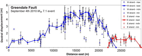
Figure 2. Displacement profile along the surface rupture of the Greendale Fault 2010 M_w 7.1 Darfield earthquake (modified from Quigley et al. 2012). Blue and red lines show displacement variations using the ‘best’ measurements for the west (W) and east (E) fault strands, respectively. The different types of measurement are: max, maximum of multiple measurements; best, preferred value from multiple measurements; indiv, one measurement; min, minimum of multiple measurements.

In addition to point sampling issues, not all paleoearthquakes on an active fault will be detected at or near the ground surface. Incompleteness of geological earthquake data, which appears to be particularly important for reverse faults (few of the faults in Table 1 are reverse), could arise because some events did not rupture the ground surface or because surface erosion or deposition processes are sufficiently fast to remove or conceal evidence of a particular surface-rupturing earthquake (e.g. McCalpin 2009; Hecker et al. 2013). One consequence of this incompleteness is that the number of active faults and potential earthquake sources may be underestimated in many regions (Wells & Coppersmith 1993; Lettis et al. 1997; Nicol et al. 2011a, 2014). In the Taranaki Rift southwest of Mount Taranaki (i.e. location of faults 7, 22 and 24; Figure 1; Table 1), for example, seismic-reflection lines reveal that ≤50% of potential active faults have resolvable surface traces (Mouslopoulou et al. 2012). Quantifying sample completeness can be achieved by estimating the minimum size of prehistoric earthquakes (e.g. slip and magnitude) we expect to be routinely resolved by the displacement of geomorphic strain markers and by examining the surface-rupture geometries of historical earthquakes in New Zealand since AD 1840 (Nicol et al. 2014). In the former case the minimum slip required to produce resolvable earthquake faulting at the ground surface varies between faults and is dependent on many factors, including the type of fault (strike slip, normal or reverse) and the rates of surface processes. On many of New Zealand's strike-slip faults, for example, recording SES <2–3 m of landforms may be challenging for all but historical earthquakes. The relationship between single-event slip and moment-magnitude data for strike-slip faults in the New Zealand National Seismic Hazard Model (Stirling et al. 2012) suggests that earthquake RI and SES information may be incomplete for events of M_w ≤ 6.9–7.2. Similarly, no reverse or strike-slip earthquakes of M_w <7.1 in the New Zealand historical catalogue have produced surface rupture (Nicol et al. 2011a, 2014; Downes & Dowrick 2014) which supports the view that, for these types of faults, surface-rupturing earthquakes of M_w <7 are unlikely. By contrast, in the thinned hot crust of the Taupo Rift (Figure 1) historical normal-fault events as low as M_w c. 5.5 may have ruptured the ground surface (Nicol et al. 2011a, 2014; Downes & Dowrick 2014), which is comparable to the minimum magnitude for surface rupture suggested by McCalpin (2009).

Incomplete sampling of the paleoearthquake record could have two important implications for earthquake parameters measured from geological data. First, in circumstances where geological data only sample larger-magnitude events that rupture the ground surface (e.g. M_w >7 events on strike-slip and reverse faults in New Zealand), these events will be quasi-characteristic (i.e. they will have a similar magnitude and SES; Schwartz & Coppersmith 1984; Wesnousky 1994). Caution should therefore be exercised when attempting to use geological paleoearthquake data to differentiate between characteristic and Gutenberg–Richter earthquake models for individual faults (see also Stein & Newman 2004). Second, because some events on each fault will not be recorded by a geological sample, these data define maximums for mean RI and SES (because more events will reduce the RI and the unsampled earthquakes are likely to have relatively small SES). There are currently insufficient data to assess how many events have been missed on the New Zealand faults sampled to date. One potential means of acknowledging this issue for paleoseismology data is to adopt the minimum magnitude of completeness (M_c) concept widely used in seismology (e.g. Wiemer & Wyss 2000). M_cg is here defined as the minimum magnitude for which all earthquakes on a fault were sampled by geological data. We propose that RI and SES for all paleoearthquake data should be quoted in concert with a minimum magnitude of completeness, although we concede that estimating M_cg may not be trivial in some cases. One approach for assigning a M_cg for SES data would be to estimate the minimum slip routinely observed in the geological record in conjunction with empirical-magnitude–SES-fault-length relationships (e.g. Wells & Coppersmith 1994; Villamor et al. 2007; Wesnousky 2008; Stirling et al. 2012, 2013), as described for strike-slip active faults earlier in this section.

Earthquake simulations

Dislocation modelling of moderate–large-magnitude earthquakes within fault systems permit the size (slip and magnitude) and RI between these synthetic events to be determined over time intervals of 10⁶ years or more (e.g. Ward 1992, 2000; Ben-Zion 1996; Fitzenz & Miller 2001; Rundle et al. 2006; Yakovlev et al. 2006; Robinson et al. 2009a, 2011; Tullis et al. 2012a, 2012b). The utility of these synthetic earthquake models is that they can be designed to replicate the regional tectonics, slip rates and geometries of real fault systems simulating 10²–10³ large-magnitude earthquakes on each fault. Our computer-generated seismicity catalogue provides a long (>10⁶ years) and complete record for more than 100 active faults in three regions of New Zealand (see Figure 1 for locations). The long duration of the earthquake simulations was adopted to provide statistically meaningful catalogues and is not intended to convey the view that the present geometries, kinematics and earthquake histories of active faults applied for >10⁶ years. Analysis of these earthquake simulations suggests that, like paleoearthquakes on active faults, synthetic events on individual faults exhibit variations in RI and SES (Robinson 2004; Robinson et al. 2009a, 2009b, 2011).

Earthquake simulations replicate static stress build-up during tectonic loading with fault failure and earthquake rupture when the fault strength is exceeded (Robinson & Benites 1996, 2001; Robinson 2004). These models have been developed for parts of the Bay of Plenty, Wellington and Marlborough regions of New Zealand (for locations see Figure 1) and consist of five key elements: (1) a geometric description of the natural faults in the region of study, which are finely divided into small cells (e.g. as small as 200 × 200 m); (2) frictional behaviour defined by a variable coefficient of friction and of static/dynamic type, with healing; (3) a driving mechanism that loads the faults toward failure; (4) fault failure based on the Coulomb Failure Criterion; and (5) fault interactions via induced changes in static stress and pore pressure. The driving mechanism results in the initial failure of one fault cell that in turn induces changes in stress/pore pressure on all other cells, on all faults. If loaded sufficiently additional cells fail as part of the same event, and the more cells that slip during a failure event the larger the magnitude of the earthquake. Once the initial conditions of the model have been specified it is therefore deterministic, not stochastic. The formulation of Okada (1992) for a uniform elastic half-space is used to calculate the induced fault displacements and their spatial derivatives and hence stresses. Induced stresses propagate through the medium at the shear-wave velocity and all faults in each model interact elastically. The model rigidity is 4.0 × 10¹⁰N m⁻² and the density 2.65 × 10³kg m⁻³, which are reasonable first approximations for the brittle crust in New Zealand (Robinson & Benites 1996, 2001). Parameters of the models are adjusted to reproduce the geologically observed long-term (> c. 10 ka) slip rates for each modelled fault and a regional b-value of c. 1.0. By contast, the earthquake RIs and SES emerge from the model and are dependent on its geometry, dynamics and rheology.

Earthquakes have been generated for a total of 119 primary normal and strike-slip faults (i.e. active faults that have been recognised by geological mapping), with slip rates of c. 0.1–25 mm a^–1 together with c. 10,000 randomly distributed additional small faults (i.e. 1–2.5 km in length; Robinson 2004; Robinson et al. 2009a, 2009b, 2011). The result is a long catalogue of about five million events with magnitudes of M_w  c. 4–8.1, which simulate a time period up to 2×10⁶ years. The earthquake populations produced by this type of model have been shown to reproduce earthquake magnitudes and RIs typical of natural faults (Somerville et al. 1999; Robinson & Benites 2001; Robinson et al. 2009a). Comparisons between geological and simulated earthquakes in this paper support this conclusion (within the uncertainties of the data) and suggest that synthetic earthquakes may approximately replicate the general form and variability of size RI and SES for geologically determined earthquakes.

Simulated earthquakes have lower M_c than geological events for the same fault (i.e. M_c of 4–5 compared to M_c of 6–7.2), which decreases the RI and SES (Tullis et al. 2012b). The importance of M_c for the recorded RI (whether it is estimated from geological or synthetic data) is illustrated in Figure 3 where values of average RI for synthetic earthquakes on the Wairau Fault increase with rising M_c. On this particular fault, the arithmetic mean RI for synthetic and geological earthquakes would be comparable if the M_cg was c. 7.15 (similar to the M_cg of 6.9–7.2 inferred for the Wairau Fault from the measurement of displaced geomorphology and the relationships between SES and magnitude for the data in Stirling et al. 2012). To facilitate the comparison of simulated and geological earthquake populations, the synthetic earthquake catalogue was sub-sampled at magnitudes greater than M_cg. For the purposes of this paper, M_cg has been estimated for simulated earthquakes by assuming that non-Gutenberg–Richter events in frequency-magnitude distributions, which rupture most (>80%) of each fault surface, would be observed at the ground surface in geological datasets. Using this criterion M_cg for reverse and strike-slip faults typically falls within the range 7.0–7.4 (i.e. 7.2 ± 0.2) and for normal faults 5.9–6.3 (6.1 ± 0.2) (Robinson et al. 2009a, 2009b, 2011). These estimates are consistent with our M_cg estimates of M_w c. 5.9–6.2 and c. 6.9–7.2 for geologically recordable slip of normal (≥0.2–0.5 m) and strike-slip faults (≥2–3 m), respectively (based on magnitude v. maximum displacement data from Stirling et al. 2012). Estimates of M_cg for geological and synthetic earthquake data are considered first-order only as, for example, they do not take account of any variability between faults or differences between the sample dimensionality of geological (point measurements) and synthetic (fault trace or surface measurements) earthquakes. We note, however, that arithmetic mean RI and SES for M_cg adjusted synthetic datasets of point samples and fault-trace measurements from the Wairau Fault are within 5%.

Figure 3. Positive relationship between the completeness magnitude (M_c) and the arithmetic mean RI for simulated earthquakes that ruptured the Wairau Fault (i.e. includes events that did not rupture the ground surface or the entire fault). Note the similarity of mean synthetic recurrence for M_cg 7.15 (c. 2200 yr) and mean recurrence for geological paleoearthquakes (2270 yr).

Data analysis

Variability of RI and SES has been assessed for paleoearthquake data using a combination of frequency histograms, probability density functions (PDF) and the coefficient of variation (Figures 4–9). Frequency histograms of RI and SES were generated for all of the faults in Table 1 using a Monte Carlo method together with the earthquake parameters and uncertainties presented in Dataset S1.

Figure 4. Recurrence interval histograms for individual active faults with seven or more recorded surface-rupturing earthquakes generated using the data in Dataset S1 and the Monte Carlo method outlined in the ‘Data analysis’ section. See Figure 1 for fault locations and Table 1 for fault details. Numbers beside fault name correlate with those assigned in Table 1 and Dataset S1.

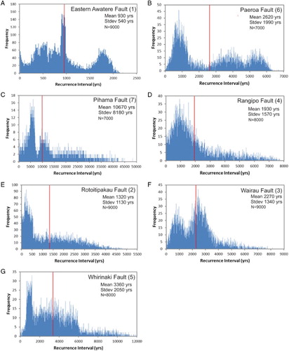
Figure 5. A, Probability density functions (PDF) for the seven faults presented in Figure 4. To enable comparison of the PDFs for faults with different mean recurrence interval, the RI curves have been normalised to their arithmetic mean (i.e. mean=1). The thick black line is the arithmetic mean of the seven faults presented. Note that for the examples presented the most common RI is typically less than or equal to the arithmetic mean, while for RI a factor of 2–4 times the mean are possible. B, RI PDFs for simulated earthquakes on six faults (Awatere, Wellington, Wairau, Wairarapa, Hope and Paeroa faults). Curve shown by the thick black line is the arithmetic mean of the curves for the individual faults. C, Mean RI PDF for geological data (red bars) plotted with best-fit log-normal and Weibull distributions. D, Average PDF for simulated RI from six faults (B) plotted with best-fit log-normal and Weibull best-fit distributions. See Figure 1 for fault locations and Table 1 for fault details.

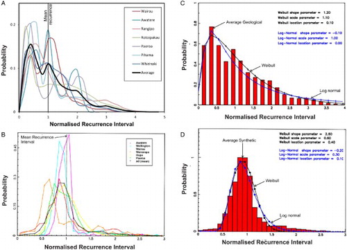
Figure 6. RI C_v variation for temporal sample windows of seven simulated earthquakes (M_c ≥ 7.5) on the Wairau Fault. Dashed line shows the mean C_v for geological data (see Table 1 and Dataset S1).

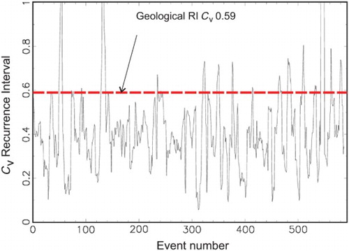
Figure 7. RI C_v histograms of A, geological earthquakes and B, synthetic earthquakes (Robinson et al. 2009a, 2009b, 2011) and C, SES of geological earthquakes.

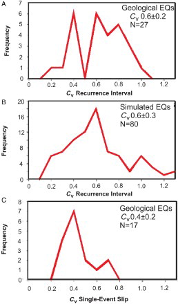
Figure 8. Histograms of SES for ten active faults with four or more recorded earthquake slip values generated using the data in Dataset S1 and the Monte Carlo method outlined in the text. Vertical lines indicate the arithmetic mean SES. For description of the faults see Table 1. Numbers beside fault name correlate with numbers assigned in Table 1 and Dataset S1.

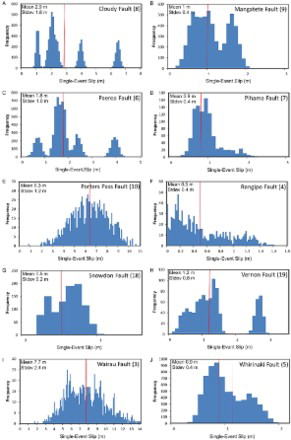
Figure 9. Histograms of SES from simulated earthquakes for five of the active faults in Table 1 including the Wairau, Paeroa and Whirinaki faults shown in Figure 8. In each case, the SES has been normalised to the arithmetic mean SES.

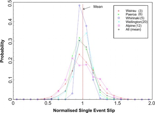
The Monte Carlo procedure is similar to that previously employed for quantifying parameters of active faults (e.g. Thompson et al. 2002; Parsons 2008). First a PDF was assigned to the timing and SES for each event identified in the geological record. The uncertainty bounds of the underpinning data are assumed to represent the 95% confidence limit of each PDF and are equally distributed about the mean; sensitivity analysis suggests that reducing the confidence limit to 75–85% does not significantly impact the results. As the probability distribution between the 95% limits is unknown, for the standard model we assume that all events in the central 95% of the distribution have equal probability. The central 95% is bounded by two 2.5% tails decreasing in probability with increasing distance from the mean (the decay being equivalent to that of a normal distribution). This standard PDF was applied to all events on all faults. It is however possible that individual events were defined by different PDFs or that all faults have approximately the same PDF which differs from the standard model. To test these possibilities we also used a normal distribution with the same 95% confidence limits as the standard model and a uniform probability model where the uncertainty bounds were equal to the 100% confidence limits. Neither of these alternative PDFs produced significantly different results compared to the standard model (i.e. mean, median and modes are within 10%) which was used for all of the histograms presented here.

The timing and slip for each event were drawn randomly from the PDFs for each parameter (RI and SES) commencing with the youngest earthquake in the sequence. Preceding (older) events randomly drawn from their PDFs were retained if they produced a positive RI (i.e. RI = age of older event—age of younger event > 0). This process was repeated until a Monte Carlo slip and timing estimate had been assigned to all earthquakes on each fault in the geological database. One thousand paleoearthquake histories (i.e. modelling all geologically recognised events on each fault 1000 times) were generated for all faults in Table 1 excluding the southern Alpine Fault. The resulting stochastic output has been plotted as histograms (e.g. Figure 4). The Monte Carlo generation of histograms was undertaken multiple times (e.g. 2–10) for the same fault. Comparison of the histograms for different runs confirmed that their general shapes do not change between runs. Given this stability, we present a single model output for each fault.

The histograms take account of the average timing and slip of events in the geological record and also reflect the measurement uncertainties in these values. The RI histograms have been used to generate PDFs for seven faults with ≥7 events (Figure 5A). To facilitate comparison of PDFs between individual faults, RI has been normalised to arithmetic mean recurrence and the vertical axis recalculated to probability. RI and SES histograms for geological earthquakes have been used in conjunction with, and compared to, histogram output for the same parameters from the earthquake simulations. Synthetic earthquake recurrence and slip populations have been presented for six of the faults in Table 1 (Figure 5B).

In addition to the frequency histograms and PDFs we have calculated the coefficient of variation for RI and SES. The coefficient of variation is a normalised measure of dispersion of a probability distribution that has been widely used in the paleoearthquake literature (e.g. Marco et al. 1996; McCalpin & Nishenko 1996; Dawson et al. 2008; Mouslopoulou et al. 2009a; Robinson et al. 2009a; Little et al. 2010; Berryman et al. 2012; Hecker et al. 2013). We follow many of these publications in assuming that RI and SES populations on individual faults are normally distributed and that C_v = standard deviation/arithmetic mean. It is acknowledged, however, that for some faults the RI may not be fit to a normal distribution (e.g. Sieh et al. 1989; Biasi et al. 2015) and the influence of a log-normal distribution on estimates of mean, standard deviation and coefficient of variation (here referred to as C_vln for log-normal distributions) are discussed in the ‘Recurrence interval’ and ‘Application to seismic hazard assessment’ sections. Coefficient of variation is a single number, which may or may not be ascribed uncertainties or described by a PDF, that is well suited to being used for comparing the variability of RI and SES between faults. C_v and C_vln for RI and SES range up to c. 2.0 (e.g. Figures 6 and 7) and indicate that earthquake parameters can vary from being purely periodic (C_v = 0) to random (C_v = 1) to clustered (C_v>1). We have derived C_v from the geological data for all of the faults in Table 1 (recurrence and slip) and for all of the simulated earthquakes (recurrence only) generated for Wellington and Taupo Rift regional models (Robinson et al. 2009a, 2009b, 2011); 12 faults have both geological and simulated earthquake records. Geological C_v carries uncertainties of one standard error which were estimated by randomly locating sample windows of duration equal to the geological record on the stochastic displacement–time curves for each fault. C_v for the earthquake simulations were derived from the M_cg-adjusted datasets.

Recurrence intervals

RI records the time between successive earthquakes on individual faults. Paleoearthquake studies indicate that RI can vary dramatically between faults and temporally on the same fault (e.g. Sieh et al. 1989; Grant & Sieh 1994; Marco et al. 1996; Dawson et al. 2003; Palumbo et al. 2004; Weldon et al. 2004; Mouslopoulou et al. 2009a; Nicol et al. 2009; also see references in Table 1 and Dataset S1). The faults in Table 1 display arithmetic mean RI over the range 130–8540 years, inversely related to fault slip rate. The lower bound of the range in RI is defined by the fastest-moving onshore faults (e.g. Hope and Alpine faults), while the upper bound is censored due to the maximum duration of the sample interval (c. 30 ka) and the requirement for four or more events. Estimates of RI for active faults in New Zealand range up to >100 ka (Stirling et al. 2012; Figure 10A), with analysis of historical earthquakes since AD 1840 suggesting that active faults of RI >10 ka may be undersampled by 50% or more (Nicol et al. 2014).

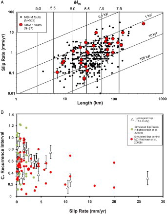
Figure 10. A, Plot of slip rate v. fault length including data from the NSHM (back small filled circles) and Table 1 (large red filled circles). Earthquake magnitude estimates from the M_w fault length empirical relationship of M_w=5.08+1.16×log(surface fault length) (Wells & Coppersmith 1994). Contours of RI of 0.1, 1, 10 and 100 ka were derived by applying the empirical data of Wells and Coppersmith (1994) for the proportional scaling between coseismic slip (D_e) and earthquake rupture length (L_e); i.e. D_e=(5×10⁻⁵)L_e. Calculations assume that each earthquake ruptured the entire fault length measured, and that all slip was coseismic slip (i.e. no interseismic fault creep occurs on timescales of thousands of years), with displacement rate (D_rate) for a given RI equal to D_e/RI or (5×10⁻⁵)L_e/RI. For a given displacement rate and fault length a mean RI can therefore be calculated. B, RI C_v vs slip rate for geological and simulated large-magnitude earthquakes (refer to key for details and text for derivation of C_v).

Frequency histograms and associated PDFs of RI provide an indication of how this parameter can vary temporally on individual faults (Figures 4, 5; Dataset S1). One of the most striking features of the frequency histograms for the geological data is the variability in their shape. This histogram variability is particularly noticeable for the faults in Dataset S1, which are constrained by the fewest number of paleoearthquakes (4–6 events). Some of the variability of RI evident in the geological data may therefore be due to the small number of events. In an attempt to address the potential sample-size issue, analysis of geological data focused on histograms and PDFs for faults with seven or more recorded paleoearthquakes (Figure 5A). Despite some variability, the histograms and PDFs in Figures 4 and 5A share common first-order geometries. These commonalities are: (1) they are often asymmetric with a long RI low-frequency tail; (2) the mode of each distribution is generally less than or equal to the mean; and (3) on average, the range in RI for each fault is about four times the mean (Figure 5A).

The shapes of the geologically derived frequency histograms and PDFs are more variable than those generated for the same faults using earthquake simulations. Figure 5B, for example, shows PDFs for synthetic earthquakes on the six faults in Figure 5A for which model outputs are available. The curves in Figure 5B are (as with the natural earthquakes) asymmetric with a mode less than the mean and a long RI tail which exceeds the mean by up to a factor of three. Unlike the natural examples, the synthetic PDFs for RI do not vary dramatically between faults. The greater stability of simulated earthquake PDFs could be due to the larger number of earthquakes underpinning these curves (compared to geological observations), the absence of uncertainty on RI in the models and/or the simulations imprecisely replicating the variability of natural faulting processes (e.g. fault strength or fault interactions). The potential impact of the short duration of the geological sample interval is illustrated in Figure 6, where RI C_v for simulated earthquakes on the Wairau Fault varies temporally from c. 0.15 to >1. The amplitudes of curves such as Figure 6 increase with decreases in the number of events in each sample window (see also Parsons 2008), supporting the view that the dispersal of RI is likely to be greater for the relatively short-duration geological samples than the earthquake simulations.

The positively skewed mean PDFs of RI for both geological and simulated earthquakes can be approximately fit by log-normal and Weibull distributions (Figure 5C, D). Both types of distributions describe the relatively low modal RI (compared to the arithmetic mean) and the long RI tail characteristic of the data. Visual inspection of the curves suggests that the Weibull distribution may fit the geological data best (Figure 5C), while the log-normal distribution better fits the simulations (Figure 5D). The difference between log-normal and Weibull distributions is small compared to the variations between PDFs for individual faults and, based on the fit to the available data, either may be appropriate for the faults examined. Weibull distributions have been reported for geological data at Pallet Creek on the San Andreas Fault (Sieh et al. 1989) and, based on analysis of waiting times to future earthquakes, are considered a better approximation than log-normal distributions for earthquake simulations on strike-slip faults throughout California (e.g. Yakovlev et al. 2006).

In cases where RI forms a log-normal distribution, its mean, standard deviation and coefficient of variation may depart from values estimated from an assumed normal distribution. For log-normal distributions, the geometric mean and multiplicative standard deviation are calculated after log transformation of the data (e.g. Limpert et al. 2001). Following back-transformation, the resulting geometric mean of RI is in years while the standard deviation (sometimes referred to as the geometric standard deviation) is a multiplicative factor. For example, the geometric mean and standard deviation for RI on the Wairau Fault are c. 1800 yr and 2.2, respectively, and the interval that covers approximately 68% of the data is c. 820 (1800/2.2) to 3960 yr (1800×2.2). The arithmetic mean and standard deviation for the Wairau Fault calculated assuming a normal distribution are c. 2270 and 1075 yr, respectively, with 68% interval 1195–3345 yr. In the case of the Wairau Fault the means and 68% interval values for normal and log-normal distributions differ by c. 20%; however, for some of the faults in Table 1 the difference is c. 50% which may be significant for some seismic-hazard assessment purposes. These differences are typically in the same sense with the geometric mean being less than the arithmetic mean and the 68% range greater for log-normal than for normal distributions.

The coefficient of variation results are consistent with the frequency histograms of RI and support the view that this parameter varies for individual faults. The coefficient of variation may also differ for normal and log-normal distributions of RI on the same fault. The variability of RI coefficient of variation calculated assuming a normal distribution (C_v) is shown on the histograms in Figure 7A, B. RI C_v for the geological data (Figure 7A) ranges from c. 0.2 to 1 with a mean of 0.6 and a standard deviation of 0.2. The observed range of RI C_v is consistent with values calculated previously from paleoearthquakes on active faults within New Zealand (e.g. Berryman et al. 2012) and internationally (e.g. Sieh et al. 1989; McCalpin & Nishenko 1996; Weldon et al. 2004; Dawson et al. 2008; Mouslopoulou et al. 2009a). They suggest that RI ranges from being quasi-periodic (e.g. c. 0.2–0.5) to quasi-random (e.g. c. 0.7–1.0). Where RI has a log-normal distribution its C_vln is only a function of the standard deviation after natural log transformation (σ_ln) and is defined as: C_vln = [exp(σ_ln²)−1]^1/2 (Limpert et al. 2001). Using this equation, C_vln for RI on the faults in Table 1 are c. 0.3–2 with an arithmetic mean of 0.9. Many of the faults displayed quasi-periodic RI (C_v and C_vln <0.5) behaviour independent of which of the two distributions was assumed. For coefficients of variation of >0.5 however, RI C_vln appears to be greater than C_v for the same fault, in some cases approaching random (C_vln = 1) or being clustered (i.e. C_vln > 1). Further detailed analysis is required to determine whether these differences are reproducible and sufficient geological RI data are available to justify assuming log-normal rather than normal distributions.

Single-event slip

SES is the slip that accrued during each surface-rupturing earthquake and, in Table 1, represents a point sample or an average from multiple point samples. Earthquake slip at the ground surface on New Zealand active faults ranges up to 18.5 m (Rodgers & Little 2006) and internationally is positively correlated to magnitude (e.g. Wells & Coppersmith 1994). The faults in Table 1 range in SES from 0.5 to 16.9 m, with the lower bound defined by the detection limit of geological investigations of normal faults. In New Zealand, SES on individual faults may be approximately uniform (Van Dissen & Nicol 2009; Little et al. 2010; Townsend et al. 2010) or vary by up to a factor of five (Nicol et al. 2010, 2011b; Townsend et al. 2010; Figure 2). Whether most faults adhere to the quasi-uniform or variable SES models, and under what geological conditions each of these models applies, are important questions (e.g. Wesnousky 1994, 2008).

Frequency histograms of SES provide an indication of how this parameter varies for ten faults in Table 1 (Figure 8). These faults provide SES for five or more surface-rupturing earthquakes and, in terms of the number of events and the completeness of the slip record, are considered to be the best of the available data. As is the case with the RI data, the shape of the histograms varies between faults. This variability of SES may be partly due to the small sample size of events and/or to the 1D sampling. Multiple modes evident for some faults (e.g. Cloudy and Paeroa faults) may, for example, directly reflect the low sample number with each mode corresponding to a specific individual event.

Histograms display a range in SES of less than a factor of c. 15; however, for the majority of the faults most of the slip events are within a factor of 2 of the mean (Figure 8). Six of the histograms (Mangatete, Pihama, Porter's Pass, Snowdon, Wairau and Whirinaki faults) have approximately normal distributions with a mean (Figure 8, red line]) that roughly coincides with the mode and a minimum approximately equal to the lower limit of recordable slip. The remaining histograms (Cloudy, Paeroa, Rangipo and Vernon) may be better approximated by log-normal distributions, although other distributions are possible given the geometries of the histograms, the small number of data and the censoring of SES that may occur towards the lower detection limit of the data.

The shapes of the geologically derived histograms are broadly consistent with those generated for the same faults using simulated seismicity. Figure 9, for example, shows PDFs for simulated earthquakes from five faults including the Wairau, Paeroa and Whirinaki faults shown in Figure 8. Slip for the simulated earthquake frequency curves are dominated by approximately normal distributions with modes approximately coincident with the mean (Figure 9). As is the case for RI data, the shapes of the synthetic histograms are less variable than those for the geological data. Again, this increase in stability could be attributed to the greater number and smaller uncertainties of earthquakes underpinning the synthetic curves and/or because these models do not entirely replicate nature. In either case more research is required to understand variability of earthquake processes.

C_v derived from the geological data for SES assuming a normal distribution is lower, and has a smaller range than, RI C_v (compare Figure 7A and C). The mean C_v for SES of 0.4 ± 0.2 is less than the c. 0.6 ± 0.2 calculated for RI and comparable to the c. 0.5 from Hecker et al. (2013), while suggesting that SES is closer to being quasi-uniform than quasi-random. Whether this quasi-uniform behaviour also applies for lower M_cg values is dependent on the magnitude–frequency earthquake distributions of the faults (e.g. characteristic or Gutenberg–Richter) and, together with the form of the SES distribution (e.g. normal or log-normal), requires further investigation (for further discussion see the following section).

Application to seismic hazard assessment

Seismic hazard analysis is one of the primary motivations for collecting and analysing paleoearthquake data. The New Zealand National Seismic Hazard model (NSHM) has been used as the hazard basis for the New Zealand Loadings Standard and for a range of other applications including assessment of infrastructural vulnerability to seismic events. Presently arithmetic mean RI and SES of large-magnitude prehistoric earthquakes on active faults are used to incorporate large-magnitude events in the NSHM. These parameters are either directly input into the model or derived from a combination of fault-slip rates and fault length using New-Zealand-specific empirical scaling relationships (Stirling et al. 2002, 2012, 2013). Inclusion of the variability of RI and SES and uncertainties in these parameters (epistemic or aleatory) for large-magnitude earthquakes is desirable and will likely be incorporated into future iterations of the NSHM (Bradley et al. 2012; Stirling et al. 2012).

The PDFs derived in the present study provide a basis for describing the variability of RI and SES in the NSHM where there are insufficient paleoearthquake data on individual faults. The PDFs for RI are commonly positively skewed with tails in the distribution comprising relatively few (e.g. <10%) long-recurrence events which will impact the hazard. In the absence of an ability to predict the timing of future large earthquakes, knowing the timing of the last event on a fault and having a PDF for RI provides a basis for estimating the probability of future fault rupture over a specified period of time (Rhoades & Van Dissen 2003; Rhoades et al. 2011; Van Dissen et al. 2013; Biasi et al. 2015). Although the RI PDF can vary between faults, the Weibull and log-normal average distributions identified in this study may be applied to active faults in the NSHM and provide a basis for examining the impact of RI variability on seismic hazard estimates.

In the absence of paleoearthquake or earthquake simulation information, C_v may be used to constrain the dispersal of RI and SES. As with PDF, C_v may change temporally on individual structures, between faults in the same system and for different types of faults (e.g. Hecker et al. 2013). One advantage of using C_v to quantify earthquake variability is that it is relatively simple to calculate and has been widely adopted in the literature for geological data and simulations in New Zealand (e.g. Robinson et al. 2009a, 2011; Little et al. 2010; Berryman et al. 2012; Biasi et al. 2015; this study) and globally (e.g. Sieh et al. 1989; McCalpin & Nishenko 1996; Weldon et al. 2004; Dawson et al. 2008; Hecker et al. 2013). However, RI data for many faults may not be normally distributed and, in these cases, C_v calculated from the standard deviation and the arithmetic mean might not provide an accurate measure of the RI dispersal. In cases where RI forms a log-normal distribution C_vln may differ significantly from C_v. Fault-specific RI C_v estimates should be used where they are available (C_v or C_vln) and may be most important for the highest slip-rate faults (e.g. Alpine Fault) which in some cases may be quasi-periodic with C_v <0.5 (Berryman et al. 2012; Biasi et al. 2015). In cases where the RI distribution is poorly constrained, a PDF of the coefficient of variation that takes account of a range of possible values may be most appropriate (see Rhoades & van Dissen 2003). Further research is required to define PDFs of the coefficient of variation and to determine under what circumstances selection of different RI distributions (e.g. normal or log-normal) are likely to influence the estimated seismic hazard.

SES data for paleoearthquakes are less numerous than those for RI. Given this paucity of data, a PDF has not been developed for SES. It is noted however that for many of the active faults the geological and simulated PDFs have approximately normal distributions. Based on the geological data, SES for those earthquakes that rupture the ground surface (and are recorded in the geological record) may be quasi-characteristic with a mean C_v of 0.4 and a standard deviation of 0.2 (Figure 7C). Hecker et al. (2013) suggest that a C_v of 0.5 is best fit by the characteristic earthquake model if the alongstrike slip variability during each event is small, but may also be approximately fit by a Gutenberg–Richter model with a M_cg ≥ 7. Given that strike-slip and reverse faults in New Zealand may have a M_cg ≥ 7, non-characteristic earthquake behaviour cannot be discounted based on the SES C_v data.

Irrespective of the techniques used to quantify earthquake variability for probabilistic seismic hazard models, it is important that geologically derived earthquake parameters are assigned a minimum magnitude of completeness (M_cg). The process of deriving a M_cg may provide insights into the sampling limitations of geological data and is also essential if the results of paleoseismic, historical seismicity and earthquake simulation studies are to be combined for hazard assessment (Tullis et al. 2012b; Hecker et al. 2013). In this study, we have not rigorously defined M_cg for all faults studied and instead provide broad indications of 7.2 ± 0.2 and 6.1 ± 0.2 for M_cg of terrestrial strike-slip faults and normal faults, respectively (refer to ‘Sampling artefacts' section). Too few data are presently available to assign M_cg values for reverse faults, however; since earthquakes on these structures are often associated with folding of the ground surface rather than fault slip, they may also be characterised by larger M_cg values (e.g. >7).

Earthquake variability and slip rates

Slip rates provide a widely utilised measure of fault size, can be combined with fault dimensions to estimate earthquake parameters and are a key input for earthquake simulations (e.g. Yakovlev et al. 2006; McCalpin 2009; Robinson et al. 2009a). Quantifying slip rates and their variation in space and time is important for understanding the potential for future earthquakes. Slip rates within fault systems are generally positively related to fault length (Bilham & Bodin 1992; Nicol et al. 1997, 2005; Mouslopoulou et al. 2009a; Cowie et al. 2012). Active faults in New Zealand from Table 1 (N = 27) and the NSHM (N = 532) show this positive relationship; however, there is significant spread in the slip rate for a given fault length (Figure 10A). Global studies of fault systems suggest that some of the spread of slip rates in Figure 10A may reflect regional changes in strain rates, with lower rates resulting in lower slip rates for faults of a given length (e.g. Nicol et al. 1997, 2005; Mouslopoulou et al. 2009a). In addition to these regional drivers, slip rates may vary according to fault location relative to other faults in a system (e.g. smaller faults in the strain shadow of larger faults may have relatively low slip rates; Nicol et al. 2005) and/or due to temporal fluctuations in RI and SES (Weldon et al. 2004; Mouslopoulou et al. 2009a; Nicol et al. 2009). Order-of-magnitude changes in slip rate from long-term average rates (e.g. 10⁵–10⁶ years) can occur due to variations in earthquake RI and, to a lesser extent, SES. These differences are most pronounced when the time interval over which the rates were measured is similar to, or less than, the arithmetic mean RI on a given fault. As the duration of the slip-rate sample increases, the rate approaches the long-term average (Mouslopoulou et al. 2009a). Over time intervals that capture six or less earthquakes (e.g. time intervals less than five times the arithmetic mean RI), the measured slip rates may not provide a reliable measure of average slip rate for hazard analysis purposes. In New Zealand, slip rates derived from displaced geomorphology typically permit measurements over time intervals up to c. 20 ka (e.g. since the Last Glacial Maximum). These data are likely to produce the most reliable slip rates for active faults with average RIs of ≤4 ka. For an RI of ≥20 ka, reliable slip rates may be difficult to estimate and the faults themselves hard to positively identify. The contribution of some of these lower-slip-rate active faults is therefore likely to be poorly defined in the NSHM (Nicol et al. 2014) and consideration should be given to including this uncertainty in the seismic hazard model.

Recent publications have suggested that the variability of RI and SES could be inversely related to fault size which, if correct, may have implications for seismic hazard assessment (e.g. Nicol et al. 2009a; Robinson et al. 2009a; Berryman et al. 2012). Many processes could contribute to the variability of earthquake parameters, including temporal changes of fault strength, fault segmentation, fault healing rate, fault loading rate and fault interactions (e.g. Wallace 1987; Stein et al. 1997; Weldon et al. 2004; Nicol et al. 2006, 2009; Robinson et al. 2009a). The notion that fault slip rate (a proxy for relative size of faults in systems) is an important factor in earthquake variability is most often founded on the view that faults interact and that stress perturbations due to slip on larger faults is more likely to advance or retard future slip on smaller faults than vice versa. In addition, it can be argued that the largest faults in some fault systems form plate boundary structures (e.g. Alpine Fault in New Zealand) and that uniform loading of these structures at plate rates (Beavan et al. 2002) will produce quasi-periodic earthquake behaviour (Berryman et al. 2012). To examine the relationship between fault slip rate and earthquake variability we plot RI C_v against fault slip rate for geological (white triangles, Figure 10B) and simulated (red and green filled circles, Figure 10B) earthquakes. Fault slip rates range in excess of two orders of magnitude (0.1–27 mm a^–1) and RI C_v from c. 0.1 to 1.25 for all synthetic and geological data (Figure 10A; Robinson et al. 2009a, 2009b). In general the geological and simulated earthquakes produce comparable distributions, although geological and simulated RI C_v may vary by up to c. 0.5 for the same fault (e.g. Vernon Fault: simulated C_v 0.1; geological C_v 0.6). A similar temporal range of RI C_v has been observed for simulated earthquakes on individual faults (e.g. Figure 6) and disparities between the two types of data could partly reflect differences in sampling rather than suggesting that either geological or simulated earthquakes are in error. Given the range of C_v observed for individual faults, it is not surprising that the plot in Figure 10B produces a broad data cloud with only a weak negative relationship between RI C_v and slip rate (i.e. faster-moving faults tend to have a lower RI C_v). Of particular note, the upper bound of the distribution appears to have a negative slope, consistent with suggestions that, on average, higher slip-rate faults have less-variable RI. The negative slope of the upper bound of the data is independent of whether RI is assumed to have a normal or log-normal distribution. The data are consistent with the notion that fault interactions could play a role in RI variability while also suggesting that other factors (e.g. sample duration, see Figure 6) probably influence the observed variability. Independent of the underlying processes the data in Figure 10B provide a basis for incorporating some slip-rate-dependent RI C_v or C_vln changes into the NSHM.

Conclusions

RIs and SES for large-magnitude earthquakes that ruptured the ground surface vary by more than an order of magnitude on individual faults. Geological and simulated earthquakes have been used to generate frequency histograms, probability density functions (PDFs) and coefficient of variation (C_v, standard deviation/arithmetic mean) values for RI and SES on New Zealand active faults. Simulated earthquakes help fill information gaps in the geological data which may arise due to measurement uncertainty, to the brevity of the record and to incompleteness of the geological sample. The shapes of histograms and PDFs generated for RIs from geological data using a Monte Carlo method are variable. RI for the best of the geological PDFs (i.e. M_w ≥7 surface-rupturing events) and the earthquake simulations are positively skewed with long recurrence tails, which are approximately described by log-normal and Weibull distributions. The geometric mean and C_vln calculated for these log-normal distributions may be up to a factor of two lower and higher, respectively, than those determined assuming a normal distribution. By contrast, SES for geological and simulated earthquakes is approximately normally distributed and appears to be less variable than RI (RI C_v 0.6 ± 0.2 geological and 0.6 ± 0.3 simulations; SES C_v 0.4 ± 0.2 geological). Variations in earthquake RI, and to a lesser extent SES, produce order-of-magnitude changes in slip rate over time intervals up to five times the mean RI. Quantifying the variability of RI, SES and slip rates is important when producing estimates of seismic hazard for surface-rupturing earthquakes, and could be estimated for active faults with poorly constrained paleoearthquake histories using the PDFs presented here.

Supplementary data

Dataset S1. Compilation of earthquake timing, recurrence interval (RI) and single-event slip (SES) for geological and historical data on New Zealand active faults, including Tables S1–S27 and Figure S1.

Table S1. Eastern Awatere Fault surface-rupturing earthquake data.

Table S2. Rotoitipakau Fault surface-rupturing earthquake data.

Table S3.Wairau Fault surface-rupturing earthquake data.

Table S4. Rangipo Fault surface-rupturing earthquake data.

Table S5. Whirinaki Fault surface-rupturing earthquake data.

Table S6. Paeroa Fault surface-rupturing earthquake data.

Table S7. Pihama Fault surface-rupturing earthquake data.

Table S8. Cloudy Fault surface-rupturing earthquake data.

Table S9. Mangatete Fault surface-rupturing earthquake data.

Table S10. Eastern Porter's Pass Fault surface-rupturing earthquake data.

Table S11. Southern Wairarapa Fault surface-rupturing earthquake data

Table S12. Alpine Fault surface-rupturing earthquake data.

Table S13. Hope Fault (Hope segment) surface-rupturing earthquake data.

Table S14. Kiri Fault surface-rupturing earthquake data.

Table S15. Lachlan Fault surface-rupturing earthquake data.

Table S16. Ngakuru Fault surface-rupturing earthquake data.

Table S17. Ohariu Fault surface-rupturing earthquake data.

Table S18. Snowdon Fault surface-rupturing earthquake data.

Table S19. Vernon Fault surface-rupturing earthquake data.

Table S20. Wellington Fault surface-rupturing earthquake data.

Table S21. Eastern Clarence Fault surface-rupturing earthquake data.

Table S22. Ihaia Fault surface-rupturing earthquake data.

Table S23. Matata Fault surface-rupturing earthquake data.

Table S24. Oaonui Fault surface-rupturing earthquake data.

Table S25. Rotohauahu Fault surface-rupturing earthquake data.

Table S26. Waimana Fault (northern) surface-rupturing earthquake data.

Table S27. Whakatane Fault (northern) surface-rupturing earthquake data.

Figure S1. Recurrence interval histograms for faults with 4–5 recorded earthquakes in Table 1 of the manuscript and not presented in Figure 4 of the manuscript. Histograms generated using the Monte Carlo method outlined in the manuscript text. The timing of surface-rupturing earthquakes on each fault are presented in Tables S1–S27.

Acknowledgements

This manuscript would not have been possible without the research of many paleoseismologists over several decades. It also benefitted greatly from insights on earthquake deformation provided by John Beavan, our colleague for nearly 20 years, and we dedicate this paper to him. Rob Langridge, Annemarie Christophersen, Matt Gerstenberger and Dan Clark are thanked for their thorough and constructive reviews of the manuscript.

Guest Editor: Dr Charles Williams.

Disclosure statement

No potential conflict of interest was reported by the authors.

Additional information

Funding

This research was mainly funded by a biennial EQC research grant (EQC Project BI10/596), by public research funding from the Government of New Zealand and funding from the Natural Hazards Research Platform.

References

- Barnes PM, Nicol A, Harrison T. 2002. Late Cenozoic evolution and earthquake potential of an active listric thrust complex, Hikurangi subduction margin, New Zealand. Geol Soc Am Bull. 114:1379–1405. doi: 10.1130/0016-7606(2002)114<1379:LCEAEP>2.0.CO;2
- Barnes PM, Pondard N. 2010. Derivation of direct on-fault submarine paleoearthquake records from high-resolution seismic reflection profiles: Wairau Fault, New Zealand. Geochem Geophys Geosy. 11:Q11013. doi:10.1029/2010GC003254.
- Bartholomew T, Little T, Clark K, Van Dissen R, Barnes P. 2014. Kinematics and paleoseismology of the Vernon Fault, Marlborough Fault System, New Zealand: implications for contractional fault bend deformation, earthquake triggering, and the record of Hikurangi subduction earthquakes. Tectonics. 33(7):1201–1218. doi:10.1002/2014TC003543.
- Beavan J, Tregoning P, Bevis B, Kato T, Meertens C. 2002. The motion and rigidity of the Pacific Plate and implications for plate boundary deformation. J Geophys Res. 107:2261. doi:10.1029/2001JB000282.
- Begg JG, Mouslopoulou V. 2010. Analysis of late Holocene faulting within an active rift using lidar, Taupo Rift, New Zealand. J Volcanol Geoth Res. 190:152–167. doi:10.1016/j.jvolgeores.2009.06.001
- Benson AM, Little TA, Van Dissen RJ, Hill N, Townsend DB. 2001. Late Quaternary paleoseismicity and surface rupture characteristics of the eastern Awatere strike-slip fault, New Zealand. Geol. Soc Am Bull. 113(8):1079–1091. doi: 10.1130/0016-7606(2001)113<1079:LQPHAS>2.0.CO;2
- Ben-Zion Y. 1996. Stress, slip and earthquakes in models of complex single-fault systems incorporating brittle and creep deformation. J Geophys Res. 101:5677–5708. doi: 10.1029/95JB03534
- Berryman KR. 1993. Age, height and deformation of Holocene marine terraces at Mahia Peninsular, Hikurangi subduction margin, New Zealand. Tectonics. 12(6):1347–1364. doi: 10.1029/93TC01542
- Berryman KR, Beanland S, Wesnousky S. 1998. Paleoseismicity of the Rotoitipakau Fault Zone, a complex normal fault in the Taupo Volcanic Zone, New Zealand. New Zeal J Geol Geophys. 41:449–465. doi: 10.1080/00288306.1998.9514822
- Berryman K, Cochran UA, Clark KJ, Biasi GP, Langridge RM, Villamor P. 2012. Major earthquakes occur regularly on an isolated plate boundary fault. Science. 336:1690. doi:10.1126/science.1218959.
- Berryman K, Villamor P, Nairn I, Van Dissen R, Begg J, Lee J. 2008. Late Pleistocene surface rupture history of the Paeroa Fault, Taupo Rift, New Zealand. New Zeal J Geol Geophys. 51:135–158. doi: 10.1080/00288300809509855
- Biasi GP, Langridge RM, Berryman KR, Clark KJ, Cochran UA. 2015. Maximum-likelihood recurrence parameters and conditional probability of a ground-rupturing earthquake on the southern alpine fault, South Island, New Zealand. B Seismol Soc Am. 105:94–106. doi:10.1785/0120130259
- Biasi GP, Weldon RJ. 2006. Estimating surface rupture length and magnitude of Paleoearthquakes from point measurements of rupture displacement. B Seismol Soc Am. 96(5):1612–1623. doi:10.1785/0120040172.
- Bilham R, Bodin P. 1992. Fault zone connectivity: slip rates and faults in the San Francisco Bay area, California. Science. 258:281–284. doi: 10.1126/science.258.5080.281
- Bradley BA, Stirling MW, McVerry GH, Gerstenberger M. 2012. Consideration and propagation of epistemic uncertainties in New Zealand probablitistic seismic-hazard analysis. B Seismol Soc Am. 102(4):1554–1568. doi:10.1785/0120140257.
- Canora-Catalán C, Villamor P, Berryman K, Martínez-Diaz JJ, Raen T. 2008. Rupture history of the Whirinaki fault, an active normal fault in the Taupo Rift, New Zealand. New Zeal J Geol Geophys. 51:277–293. doi: 10.1080/00288300809509866
- Cowan HA. 1990. Late Quaternary displacements on the hope fault at Glyn Wye, North Canterbury. New Zeal J Geol Geophys. 33:285–293. doi: 10.1080/00288306.1990.10425686
- Cowan HA, McGlone MS. 1991. Late Holocene displacements and characteristic earthquakes on the Hope River segment of the Hope Fault, New Zealand. J Roy Soc New Zeal. 21(4):373–384. doi: 10.1080/03036758.1991.10420834
- Cowie PA, Roberts GP, Bull JM, Visini F. 2012. Relationships between fault geometry, slip rate variability and earthquake recurrence in extensional settings. Geophys J Int. doi:10.1111/j.1365-246X.2012.05378.x
- Dawson TE, McGill SF, Rockwell TK. 2003. Irregular recurrence of paleoearthquakes along the central Garlock Fault near El Paso Peaks, California. J Geophys Res: Solid Eart. 108(B7):2356. doi:10.1029/2001JB001744.
- Dawson TE, Weldon RJ, Biasi GP. 2008. Appendix B. Recurrence interval and event age data for Type A faults. USGS Open File Report 2007-1437B; CGS Special Report 203B; SCEC Contribution #1138B. In: WGCEP. The UNIFORM California Earthquake Rupture Forecast, version 2. Reston, VA: USGS; [cited 2016 Feb 10]. Available from: http://pubs.usgs.gov/of/2007/1437/b/
- Downes GL, Dowrick DJ. 2014. Atlas of isoseismal maps of New Zealand earthquakes, 1843–2003. 2nd ed. Institute of Geological and Nuclear Sciences Monograph 25 [CD]. Lower Hutt: Institute of Geological and Nuclear Sciences.
- Fitzenz D, Miller S. 2001. A forward model for earthquake generation on interacting faults including tectonics, fluids, and stress transfer. J Geophys Res. 106:26689–26,706. doi: 10.1029/2000JB000029
- Friedrich AM, Wernicke BP, Niemi NA, Bennett RA, Davis JL. 2003. Comparison of geodetic and geologic data from the Wasatch region, Utah, and implications for the spectral character of Earth deformation at periods of 10 to 10 million years. J Geophys Res. 108(B4):2199. doi:10.1029/2001JB000682, 2003.
- Grant LB, Sieh K. 1994. Paleoseismic evidence of clustered earthquakes on the San Andreas fault in the Carrizo Plain, California. J Geophys Res. 99:6819–6841. doi: 10.1029/94JB00125
- Hecker S, Abrahamson NA, Wooddell KE. 2013. Variability of displacement at a point: implications for earthquake-size distribution and rupture hazard on faults. B Seismol Soc Am. 103(A2):651–674. doi:10.1785/0120120159.
- Hemphill-Haley MA, Weldon RJ. 1999. Estimating prehistoric earthquake magnitude from point measurements of surface rupture. B Seismol Soc Am. 89(5):1264–1279.
- Heron D, Van Dissen R, Sawa M. 1998. Late Quaternary movement on the Ohariu Fault, Tongue Point to MacKays Crossing, North Island, New Zealand. New Zeal J Geol Geophys. 41:419–439. doi: 10.1080/00288306.1998.9514820
- Howard M, Nicol A, Campbell JK, Pettinga JR. 2005. Prehistoric earthquakes on the strike-slip Porters Pass Fault, Canterbury, New Zealand. New Zeal J Geol Geophys. 48:59–74. doi: 10.1080/00288306.2005.9515098
- Howarth JD, Fitzsimons SJ, Norris RJ, Jacobsen GE. 2014. Lake sediments record high intensity shaking that provides insight into the location and rupture length of large earthquakes on the Alpine Fault, New Zealand. Earth Planet Sc Lett. 403:340–351. doi: 10.1016/j.epsl.2014.07.008
- Langridge RM, Van Dissen R, Rhoades D, Villamor P, Little T, Litchfield N, Clark K, Clark D. 2011. Five thousand years of surface ruptures on the Wellington Fault, New Zealand: implications for recurrence and fault segmentation. B Seismol Soc Am. 101(5). doi:10.1785/0120100340.
- Lettis WR, Wells DL, Baldwin JN. 1997. Empirical observations regarding reverse earthquakes, Blind thrust faults and Quaternary deformation: are blind thrust faults truly blind? B Seismol Soc Am. 87(5):1171–1198.
- Limpert E, Stahel WA, Abbt M. 2001. Log-normal distributions across the sciences: keys and clues. BioScience. 51(5):341–352. doi: 10.1641/0006-3568(2001)051[0341:LNDATS]2.0.CO;2
- Litchfield N, Van Dissen R, Hemphill-Haley M, Townsend D, Heron D. 2010. Post c. 300 year rupture of the Ohariu Fault in Ohariu Valley, New Zealand. New Zeal J Geol Geophys. 53:43–56. doi: 10.1080/00288301003631780
- Litchfield N, Van Dissen R, Heron D, Rhoades D. 2006. Constraints on the timing of the three most recent surface rupture events and recurrence interval for the Ohariu Fault: trenching results from MacKays Crossing, Wellington, New Zealand. New Zeal J Geol Geophys. 49:57–61. doi: 10.1080/00288306.2006.9515147
- Litchfield NJ, Van Dissen R, Sutherland R, Barnes PM, Cox SC, Norris R, Beavan J, Langridge R, Villamor P, Berryman K, et al. 2014. A model of active faulting in New Zealand. New Zeal J Geol Geophys. 57(1):32–56. doi:10.1080/00288306.2013.854256.
- Little TA, Van Dissen R, Rieser U, Smith EGC, Langridge RM. 2010. Coseismic strike slip at a point during the last four earthquakes on the Wellington fault near Wellington, New Zealand. J Geophys Res. 115:B05403. doi:10.1029/2009JB006589, 2010.
- Little TA, Van Dissen R, Schermer E, Carne R. 2009. Late Holocene surface ruptures on the southern Wairarapa fault, New Zealand: link between earthquakes and the uplifting of beach ridges on a rock coast. Lithosphere. 1:4–28. doi:10.1130/L7.1.
- Marco S, Stein M, Agnon A. 1996. Long-term earthquake clustering: a 50,000-year paleoseismic record in the Dead Sea Graben. J Geophys Res. 101(B3):6179–6191. doi: 10.1029/95JB01587
- Mason D, Little TA, Van Dissen RJ. 2006. Refinements to the paleoseismic chronology of the eastern Awatere Fault from trenches near Upcot Saddle, Marlborough, New Zealand. New Zeal J Geol Geophys. 49:383–397. doi: 10.1080/00288306.2006.9515175
- McCalpin JP, editor. 2009. Paleoseismology. 2nd ed. International Geophysics Series 95. Elsevier Publishing.
- McCalpin JP, Nishenko SP. 1996. Holocene paleoseismicity, temporal clustering, and probabilities of future large (M>7) earthquakes on the Wasatch fault zone, Utah. J Geophys Res. 101:6233–6253.
- Mouslopoulou V. 2006. Quaternary geometry, kinematics and paleoearthquake history at the intersection of the strike-slip North Island Fault System and Taupo Rift, New Zealand [PhD thesis]. Wellington: Victoria University of Wellington.
- Mouslopoulou V, Nicol A, Little TA, Begg JG. 2009a. Paleoearthquake surface rupture in a transition zone from strike-slip to oblique-normal slip and its implication to seismic hazard, North Island Fault System, New Zealand. In: Historical and pre-historical records of earthquake ground effects for seismic hazard assessment. Geological Society, London, Special Publication. 316:269–292. doi:10.1144/SP316.17.
- Mouslopoulou V, Nicol A, Walsh JJ, Begg J, Townsend D, Hristopulos DT. 2012. Fault-slip accumulation in an active rift over thousands to millions of years and the importance of paleoearthquake sampling. J Struc Geol. 36:71–80. doi:10.1016/j.jsg.2011.11.010.
- Mouslopoulou V, Walsh JJ, Nicol A. 2009b. Fault displacement rates on a range of timescales. Earth Planet Sc Lett. 278:186–197. doi: 10.1016/j.epsl.2008.11.031
- Nicol A, Begg J, Mouslopoulou V, Stirling M, Townsend D, Van Dissen R, Walsh J. 2011a. Active faults in New Zealand: what are we missing? In: Litchfield NJ, Clark K, editors. Abstract volume. Geosciences 2011: annual conference of the Geoscience Society of New Zealand; 2011 Nov 27–Dec 1; Nelson, New Zealand. Geoscience Society of New Zealand Miscellaneous Publication 130A:79.
- Nicol A, Langridge R, Van Dissen R. 2011b. Wairau fault: late quaternary displacements and paleoearthquakes. Field trip 1. In: Lee JM, editor. Field trip guides. Geosciences 2011: annual conference of the Geoscience Society of New Zealand; 2011 Nov 27–Dec 1; Nelson, New Zealand. Geoscience Society of New Zealand miscellaneous publication 130B.
- Nicol A, Van Dissen R, Stirling M, Gerstenberger M. 2014. Implications of historical large magnitude earthquakes for the incompleteness of New Zealand's prehistorical earthquake record. In: Holt KA, editor. Abstract volume. Geosciences 2014: annual conference of the Geoscience Society of New Zealand; 2014 Nov 24–27; New Plymouth, New Zealand. Geoscience Society of New Zealand Miscellaneous Publication 139A:79.
- Nicol A, Villamor P, Berryman K, Walsh J. 2007. Variable paleoearthquake recurrence intervals arising from fault interactions, Taupo Rift, New Zealand. In: Ubertini L, Manciola P, Casadei S, Grimaldi S, complilers. Earth: our changing planet. Proceedings of the International Union of Geodesy and Geophysics XXIV; 2007 Jul 2–13; Perugia, Italy.
- Nicol A, Walsh JJ, Berryman K, Villamor P. 2006. Interdependence of fault displacement rates and paleoearthquakes in an active rift. Geology. 34:865–868. doi: 10.1130/G22335.1
- Nicol A, Walsh J, Manzocchi T, Morewood N. 2005. Displacement rates and average earthquake recurrence intervals on normal faults. J Struc Geol. 27:541–551. doi: 10.1016/j.jsg.2004.10.009
- Nicol A, Walsh JJ, Mouslopoulou V, Villamor P. 2009. Earthquake histories and an explanation for Holocene acceleration of fault displacement rates. Geology. 37(10):911–914. doi:10.1130/G25765A.
- Nicol A, Walsh JJ, Villamor P, Seebeck H, Berryman KR. 2010. Normal fault interactions, paleoearthquakes and growth in an active rift. J Struc Geol. 32:1101–1113. doi:10.1016/j.jsg.2010.06.018.
- Nicol A, Walsh JJ, Watterson J, Underhill J. 1997. Displacement rates of normal faults. Nature. 390:157–159. doi: 10.1038/36548
- Okada Y. 1992. Internal deformation due to shear and tensile faults in a half-space. B Seismol Soc Am. 82:1018–1040.
- Ota Y, Beanland S, Berryman KR, Nairn IA. 1988. The Matata fault: active faulting at the north-western margin of the Whakatane Graben, Eastern Bay of Plenty. Research Notes, New Zealand Geological Survey Record. 35:6–13.
- Palumbo L, Benedetti L, Bourles D, Cinque A, Finkel R. 2004. Slip history of the Magnola fault (Appennines, Central Italy) from 36Cl surface exposure dating: evidence for strong earthquakes over the Holocene. Earth Planet Sc Lett. 225:163–176. doi: 10.1016/j.epsl.2004.06.012
- Parsons T. 2008. Monte Carlo method for determining earthquake recurrence parameters from short paleoseismic catalogs: example calculations from California. J Geophys Res. 113(B03302). doi:10.1029/2007JB004998,2008.
- Pondard N, Barnes PM. 2010. Structure and paleoearthquake records of active submarine faults, Cook Strait, New Zealand: implications for fault interactions, stress loading, and seismic hazard. J Geophys Res. 115(B12320). doi:10.1029/2010JB007781.
- Quigely M, Van Dissen R, Litchfield N, Villamor P, Duffy B, Barrell D, Furlong K, Stahl T, Bilderback E, Noble D. 2012. Surface rupture during the 2010 Mw 7.1 Darfield (Canterbury) earthquake: implications for fault rupture dynamics and seismic-hazard analysis. Geology. 40(1):55–58. doi:10.1130/G32528.
- Rhoades DA, Van Dissen RJ. 2003. Estimates of the time-varying hazard of rupture of the Alpine Fault, New Zealand, allowing for uncertainties. New Zeal J Geol Geophys. 46(4):479–488. doi:10.1080/00288306.2003.9515023.
- Rhoades DA, Van Dissen RJ, Langridge RM, Little TA, Ninis D, Smith EGC, Robinson R. 2011. Re-evaluation of conditional probability of rupture of the Wellington-Hutt Valley segment of the Wellington Fault. Bulletin of the New Zealand Society for Earthquake Engineering. 44(2):77–86.
- Robinson R. 2004. Potential earthquake triggering in a complex fault network: The Northern South Island, New Zealand. Geophys J Int. 159:734–748. doi: 10.1111/j.1365-246X.2004.02446.x
- Robinson R, Benites R. 1996. Synthetic seismicity models for the Wellington region, New Zealand: implications for the temporal distribution of large events. J Geophys Res. 101:27833–27845. doi: 10.1029/96JB02533
- Robinson R, Benites R. 2001. Upgrading a synthetic seismicity model for more realistic fault ruptures. Geophys Res Lett. 28:1843–1846. doi: 10.1029/2000GL012300
- Robinson R, Nicol A, Walsh JJ, Villamor P. 2009a. Features of earthquake occurrence in a complex normal fault network: results from a synthetic seismicity model of the Taupo Rift, New Zealand. J Geophys Res. 114:B12306. doi:10.1029/2008JB006231.
- Robinson R, Van Dissen R, Litchfield N. 2009b. It's our fault—synthetic seismcity of the Wellington region: final report. GNS Science Consultancy Report 2009/192. Lower Hutt: GNS Science.
- Robinson R, Van Dissen R, Litchfield N. 2011. Using synthetic seismicity to evaluate seismic hazard in the Wellington region, New Zealand. Geophys J Int. 187:510–528. doi:10.1111/j.1365-246X.2011.05161.x
- Rodgers DW, Little TA. 2006. World's largest coseismic strike-slip offset: the 1855 rupture of the Wairarapa Fault, New Zealand, and implications for displacement/length scaling of continental earthquakes. J Geophys Res. 111:B12408. doi:10.1029/2005JB004065.
- Rundle P, Rundle J, Tiampo K, Donnellan A, Turcotte D. 2006. Virtural California: fault model, frictional parameters, applications. Pure Appl Geophys. 163:1819–1846. doi: 10.1007/s00024-006-0099-x
- Schwartz DP, Coppersmith KJ. 1984. Fault behavior and characteristic earthquakes: examples from the Wasatch and San Andreas Fault zones. J Geophys Res. 89:5681–5698. doi:10.1029/JB089iB07p05681.
- Stein R, Barka A, Dieterich J. 1997. Progressive failure on the North Anatolian Fault since 1939 by earthquake stress triggering. Geophys J Int. 128:594–604. doi: 10.1111/j.1365-246X.1997.tb05321.x
- Stein S, Newman A. 2004. Characteristic and uncharacteristic earthquakes as possible artifacts: applications to the New Madrid and Wabash seismic zones. Seismol Res Lett 75:173–187. doi: 10.1785/gssrl.75.2.173
- Sieh KE, Stuiver M, Brillinger D. 1989. A more precise chronology of earthquakes produced by the San Andreas fault in southern California. J Geophys Res. 94:603–623. doi: 10.1029/JB094iB01p00603
- Somerville P, Irikura K, Graves R, Sawada S, Wald D, Abrahamson N, Iwasaki Y, Kagawa T, Smith N, Kowada A. 1999. Characterizing crustal earthquake slip models for the prediction of strong ground motion. Seismol Res Lett. 70:59–80. doi: 10.1785/gssrl.70.1.59
- Stirling MW, McVerry GH, Berryman KR. 2002. A new seismic hazard model for New Zealand. B Seismol Soc Am. 92:1878–1903. doi: 10.1785/0120010156
- Stirling M, McVerry G, Gerstenberger M, Litchfield N, Van Dissen R, Berryman K, Barnes P, Wallace L, Villamor P, Langridge R, et al. 2012. National Seismic Hazard model for New Zealand: 2010 Update. B Seismol Soc Am. 102(4):1514–1542. doi:10.1785/0120110170.
- Stirling MW, Goded T, Berryman KR, Litchfield NJ. 2013. Selection of earthquake scaling relationships for seismic hazard analysis. B Seismol Soc Am. 103(6):2993–3011. doi:10.1785/0120130052.
- Thompson SC, Weldon RJ, Rubin CM, Abdrakhmatov K, Molnar P, Berger GW. 2002. Late quaternary slip rates across the central Tien Shan, Kyrgyzstan, Central Asia. J Geophys Res, B, Solid Eart and Planets. 107(B9):2203. doi:10.1029/2001JB000596.
- Townsend D, Nicol A, Mouslopoulou V, Begg JG, Beetham RJ, Clark D, Giba M, Heron D, Lukovic B, Macphearson A, et al. 2010. Paleoearthquake histories of a normal fault system in the southwestern Taranaki Peninsula, New Zealand. New Zeal J Geol Geophys. 53(4):375–394. doi: 10.1080/00288306.2010.526547
- Tullis TE, Richards-Dinger K, Barall M, Dieterich JH, Field EH, Heien EM, Kellogg LH, Pollitz FF, Rundle JB, Sachs MK, et al. 2012a. Generic earthquake simulator. Seismol Res Lett. 83(6):959–963. doi: 10.1785/0220120093
- Tullis TE, Richards-Dinger K, Barall M, Dieterich JH, Field EH, Heien EM, Kellogg LH, Pollitz FF, Rundle JB, Sachs MK, et al. 2012b. A comparison among observations and earthquake simulator results for the allcal2 California fault model. Seismol Res Lett. 83(6):994–1006. doi: 10.1785/0220120094
- Van Dissen RJ, Nicol A. 2009. Mid-late Holocene paleoseismicity of the middle Clarence valley section of the Clarence Fault, Marlborough, New Zealand. New Zeal J Geol Geophys. 52:195–208. doi: 10.1080/00288300909509886
- Van Dissen R, Rhoades D, Little T, Litchfield N, Carne R, Villamor P. 2013. Conditional probability of rupture of the Wairarapa and Ohariu faults, New Zealand. New Zeal J Geol Geophys. 56:53–67. doi: 10.1080/00288306.2012.756042
- Villamor P, Van Dissen RJ, Alloway BV, Palmer AS, Litchfield NJ. 2007. The Rangipo Fault, Taupo rift, New Zealand: an example of temporal slip-rate and single-event displacement variability in a volcanic environment. Bull Geol Soc Am. 119:529–547. doi: 10.1130/B26000.1
- Wallace RE. 1987. Grouping and migration of surface faulting and variations in slip rates on faults in the Great Basin Province. B Seismol Soc Am. 77:868–876.
- Ward SN. 1992. An application of synthetic seismicity in earthquake statistics: the Middle America Trench. J Geophys Res. 97:6675–6682. doi: 10.1029/92JB00236
- Ward S. 2000. San Francisco Bay Area earthquake simulations: a step toward a standard physical earthquake model. B Seismol Soc Am. 90:370–386. doi: 10.1785/0119990026
- Weldon R, Scharer K, Fumal T, Biasi G. 2004. Wrightwood and the earthquake cycle: what a long recurrence record tells us about how faults work. GSA Today. 14(9):4–10. doi: 10.1130/1052-5173(2004)014<4:WATECW>2.0.CO;2
- Wells A, Yetton MD, Duncan RP, Stewart GH. 1999. Prehistoric dates of the most recent Alpine fault earthquakes, New Zealand. Geology. 27:995–998. doi: 10.1130/0091-7613(1999)027<0995:PDOTMR>2.3.CO;2
- Wells A, Goff J. 2007. Coastal dunes in Westland, New Zealand, provide a record of paleoseismic activity on the Alpine fault. Geology. 35:731–734. doi:10.1130/G23554A.1.
- Wells DL, Coppersmith KJ. 1993. Likelihood of surface rupture as a function of magnitude. Seismol Res Lett. 64:54.
- Wells DL, Coppersmith KJ. 1994. New empirical relationships among magnitude, rupture length, rupture width, rupture area, and surface displacement. B Seismol Soc Am. 84:974–1002.
- Wesnousky S. 1994. The Gutenberg-Richter or characteristic earthquake distribution, which is it? B Seismol Soc Am. 84:1940–1959.
- Wesnousky SG. 2008. Displacement and geometrical characteristics of earthquake surface ruptures: Issues and implications for seismic-hazard analysis and the process of earthquake rupture. B Seismol Soc Am. 98(4):1609–1632. doi: 10.1785/0120070111
- Wiemer S, Wyss M. 2000. Minimum magnitude of completeness in earthquake catalogs: examples from Alaska, the Western United States, and Japan. B Seismol Soc Am. 90(4):859–869. doi: 10.1785/0119990114
- Xu X, Deng Q. 1996. Nonlinear characteristics of paleoseismicity in China. J Geophys Res. 101:6209–6231. doi: 10.1029/95JB01238
- Yakovlev G, Turcotte DL, Rundle JB, Rundle PB. 2006. Simulation-based distributions of earthquake recurrence times on the San Andreas Fault System. B Seismol Soc Am. 96:1995–2007. doi:10.1785/0120050183.
- Yetton M, Wells A. 2010. Earthquake rupture history of the Alpine fault over the last 500 years. In: Williams et al., editors. Geologically active. London: Taylor and Francis Group; p. 881–891.
- Zacheriasen J, Berryman K, Langridge R, Prentice C, Rymer M, Stirling M, Villamor P. 2006. Timing of late Holocene surface rupture of the Wairau fault, Marlborough. New Zeal J Geol Geophys. 49:159–174. doi: 10.1080/00288306.2006.9515156