Probing the subsurface of the Auckland Volcanic Field with ambient seismic noise

ABSTRACT

Current understanding of the Auckland Volcanic Field is predominantly based on geological and geochemical observations from the surface. Low local seismicity hinders passive seismic imaging efforts, whereas strong shallow heterogeneity reduces the resolution and penetration of active seismic models. To overcome these difficulties, we have estimated crustal shear-wave velocity profiles beneath the Auckland Volcanic Field from the ocean-generated ambient seismic noise. Variations in seismic velocity in the shallow crust correlate with variations in surface geology. In addition, our results highlight a contrast between oceanic and continental features in the Auckland Volcanic Field. Velocity models associated with the Waipapa Terrane (relative juvenile continental crust) tend to show a mid-crustal low-velocity anomaly, whereas a monotonic increase in velocity is associated with including the oceanic rocks in the ophiolite belt of the Dun Mountain–Maitai Terrane.

KEYWORDS:

• Auckland Volcanic Field
• Dun Mountain–Maitai Terrane
• ambient seismic noise
• tomography
• crustal structure
• New Zealand

Introduction

The active Auckland Volcanic Field (AVF) coincides with the most highly populated urban area of New Zealand and consists of more than 50 volcanoes (Hayward et al. 2011). In recent years, efforts have been made to improve geological knowledge about the field, so that volcanic risk can be better assessed and civil defence measures can be improved. A large amount of information on the history and mechanisms of eruptions has been collected and published by university and government institutions under the DEVORA (Determining Volcanic Risk in Auckland) project (Bebbington & Cronin 2011; Lindsay et al. 2011; McGee et al. 2013; Kereszturi et al. 2014). Structural information about the lithosphere under the AVF is crucial for understanding controls on eruptions, but data are scarce compared with those available for the other major cities in New Zealand. Perhaps this is because cities such as Christchurch and Wellington face more immediate risks of another kind, in the form of earthquakes.

Low levels of natural seismicity and high levels of ambient seismic noise of Auckland mean that seismometers in the region receive little in terms of local seismic signals to investigate the subsurface, hindering many conventional passive seismic imaging techniques. The few geophysical studies that have been made of the AVF have either produced relatively high-resolution two-dimensional images of the first few kilometres of the subsurface (Eccles et al. 2005; Davy 2008) or penetrated to greater depths at the expense of resolution (Stern et al. 1987; Horspool et al. 2006; Ashenden et al. 2011).

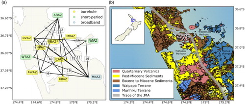
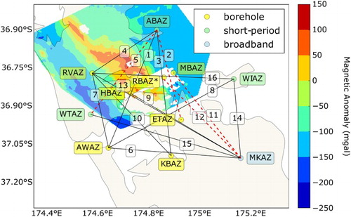
Seismic data from the Auckland Volcano Seismic Network (AVSN, Figure 1a) are publicly available through the GeoNet project (GeoNet 2001). The AVSN was installed to detect volcanic tremor and to possibly image the lithosphere with distant earthquakes. We used seismic data from six short-period borehole seismometers, three short-period surface seismic stations, and one broadband seismometer. Data from a seventh short-period borehole seismometer (RBAZ, Figure 1a), installed on Rangitoto Island by the University of Auckland, has been added for this study.

Figure 1. (a) Map of the Auckland area with the seismic network and numbered paths defined by station pairs used in this study. *University of Auckland seismometer. (b) Geological map (modified after Kermode & Heron 1992) including the Auckland Volcanic Field (AVF) and exposures of the Murihiku Terrane to the south.

Much of the seismic noise that the Auckland region experiences is generated by ocean waves, because of the proximity of extensive and intricate coastlines (Tindle & Murphy 1999; Gorman et al. 2003; Behr et al. 2013). This ambient noise can be exploited as a passive seismic source. Ambient seismic noise has been successfully used internationally to produce subsurface models of intermediate spatial resolution and penetration depth (Lin et al. 2008; Pyle et al. 2010; Stankiewicz et al. 2010, 2012; Saygin & Kennett 2012; Young et al. 2013) and in New Zealand (Lin et al. 2007; Behr et al. 2010, 2011). Horspool et al. (2006) used a joint inversion of teleseismic receiver functions and surface-wave phase velocities to determine the shear-wave velocity structure in the crust and upper mantle beneath station MKAZ at Moumoukai in the Hunua Ranges (Figure 1a). We present the first seismic images of the AVF subsurface that reveal structure in the entire crustal package and account for lateral heterogeneity.

In the following, we first present a brief overview of the geological framework of the region, then describe the instrumentation and data acquisition, the methods of data processing and present the results in terms of seismic images. Finally, we discuss possible subsurface geologic implications for the Auckland region that can be deduced from our results.

Geological framework

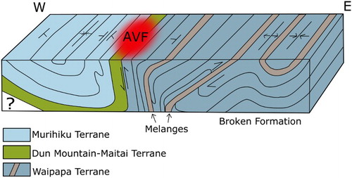
The basement rocks of the Auckland region were accreted to the Gondwana supercontinent from the late Paleozoic to at least mid-Cretaceous and can be divided into three belts (Figure 2), from east to west: (1) the imbricated, mainly Mesozoic age Waipapa Terrane, dominated by highly deformed terrigenous clastics with melange and broken formation structure (Spörli et al. 1989; Adams et al. 2009); (2) the mostly late Paleozoic Dun Mountain–Maitai Terrane, containing the Dun Mountain ultramafic belt (Eccles et al. 2005; Williams et al. 2006), with possibly a sliver of Caples Terrane to the east (Spörli et al. 2015); and (3) the Murihiku Terrane of gently folded Mesozoic sedimentary rocks (Briggs et al. 2004) that are of significantly lower metamorphic grade than those of the Waipapa Terrane, which ranges up to pumpellyite–actinolite. There are no schists and intrusive felsic rocks exposed at the surface. The Dun Mountain–Maitai Terrane is concealed by younger cover sequences, but its serpentinite shear zones can be detected magnetically as the Junction Magnetic Anomaly (JMA; Hatherton & Sibson 1970; Eccles et al. 2005). A coinciding local gravity anomaly indicates the presence of a large lensoid body of crystalline ultramafic rocks (Williams et al. 2006). The deeper configuration of the covered Dun Mountain–Maitai Terrane can only be inferred from along-strike analogous exposures throughout New Zealand (Eccles et al. 2005): We extrapolate this to be a steeply east-dipping band that may turn to sub-horizontal towards the west at depth (Figure 2).

Figure 2. Schematic representation of the expected crustal structure under the greater Auckland area, from the surface to the base of the lithosphere, after Eccles et al. (2005). Not to scale. Brown: thin ocean floor slivers marking the base of thrust slices of broken formation terrigenous clastics in the accreted Waipapa Terrane. Depth extent is only speculative, but would not be valid at and below the brittle/ductile boundary (c. 10 km depth).

From 85 Ma (mid–Late Cretaceous) to 52 Ma (early Eocene), the continent of Zealandia separated from Gondwana (Bache et al. 2014) and the tectonic regime changed from convergence to extension, resulting in considerable crustal thinning. The basement rocks were initially uplifted and eroded, but eventually subsided and became covered discordantly by a sequence of Tertiary sedimentary rocks, including the Te Kuiti Group (Edbrooke et al. 2003). Convergent tectonics resumed in the Miocene, when the presently active plate boundary propagated through New Zealand and arc volcanism above a subduction zone resumed, in the Auckland region leading to the formation of the Waitemata turbidite basin and its bounding chains of arc volcanoes (Hayward 1993). However, after the Miocene, the plate boundary activity migrated eastward to its present location in the Taupo Volcanic Zone (Mortimer et al. 2010), leaving the Auckland region and Northland in a less-active behind-arc position, with renewed extensional tectonics and small scale basaltic volcanism, of which the AVF is an example. The active AVF is a typical monogenetic field (Smith et al. 2008) composed of many small volcanoes (Hayward et al. 2011), many of which have erupted only once. The basaltic magma is considered to originate in the asthenospheric mantle at 60–100 km depth (McGee et al. 2013) and rises directly to the surface without forming crustal magma chambers.

Auckland City lies in a depression influenced by the pattern of geological units (Figure 1b) and sculpting of the landscape by sea-level changes during the Pleistocene (Hayward et al. 2011). The depression is filled with young cover rocks, the most voluminous of which are the Miocene Waitemata Group (Edbrooke et al. 2003; Kenny et al. 2012). To the east is a belt of north–northwest-striking ranges with exposed Waipapa Terrane basement, while rugged ranges in the west expose Miocene arc volcanics with a particular abundance of dense rocks.

Together with the basement in all of eastern Zealandia, the crust under Auckland is less evolved than normal continental crust. During the Mesozoic convergent tectonics, these rocks always occupied a relatively frontal position in the accretionary prism. Present-day Taiwan (Camanni et al. 2016) represents a similar example. This eastern crust never experienced the large-scale deep recycling into plutons and gneisses that are prevalent in western Zealandia and equivalent belts in Australia (Sutherland 1999; Daczko et al. 2001). Because of this, the Auckland crust may also have been somewhat thinner from the outset, before additional thinning during the Late Cretaceous–early Paleogene extension. Obtaining more data on the structure of this crust is not only helpful for volcanic risk assessment, but will also provide a good illustration of the structure in such relatively juvenile crust.

Method

Ambient noise tomography (ANT) is a three-stage method that can be used to interrogate the subsurface. ANT has been widely successful and often resolves structures in the upper crust at a higher resolution than earthquake-based surface wave tomography (Shapiro et al. 2005; Yao et al. 2006; Lin et al. 2008). The first stage involves cross-correlating ambient seismic noise—typically ocean waves causing weak seismic vibrations—on pairs of stations in the AVF. Under the right conditions, this provides an estimate of the surface-wave impulse response between these stations (Shapiro & Campillo 2004; Snieder 2004; Larose et al. 2006).

In the second stage, the group and phase velocity of the surface wave information from stage one are estimated as a function of period. The penetration depth of surface waves is proportional to their wavelength so heterogeneous media give rise to dispersion. The final stage involves the inverse problem of making inferences about the shear-wave velocity profile, given the observed frequency dependence of phase and group surface wave velocity.

The cross-correlations of stage 1 were performed in the software package MSNoise (Lecocq et al. 2014). These cross-correlation functions (CCFs) stem from the cross-correlation of 30-minute waveforms summed to form a single daily CCF. We used single-bit normalisation to remove earthquake generated signal (See Table B.1 in Ensing 2015 for the parameters and full configuration details). The sum of CCFs converges after 200 days to a stable estimate of the surface wave impulse response for the 16 station pairs analysed for this study.

We obtained dispersion relations in stage 2 for both group and phase velocities of the surface waves by applying multiple band-pass filters (Herrmann 1973) to the impulse response in the frequency domain (Cooley & Tukey 1965) using do_mft from Computer Programs in Seismology (Herrmann 2013). Computer Programs in Seismology’s do_mft allows for a number of different input parameters. We set the units to counts, the type to Rayleigh, and the filter parameter α to 3.00 and 6.25 for the inter-station distances <50 and 50–65 km respectively (after Cho et al. 2007). The filter parameter, α, is related to the inter-station distance and helps balance a resolution trade-off between the time and frequency domains (Herrmann 1973). We performed multiple filter analysis on periods of 1–15 s because this included our highest energy band or the highest spectral amplitudes.

For stage 3, the inverse problem, we iteratively perturbed the velocity model and compared the fit between the predicted dispersion data for the perturbed model and the observed dispersion data using surf96 from ‘Computer Programs in Seismology’ (Herrmann 2013). We used an initial model of 32 isotropic layers that extends from 0–25 km, with several thin layers concentrated near the surface and layer thickness increasing with depth because our power to resolve decreases with depth. The first kilometre was given three layers (0.2, 0.3 and 0.5 km thick), then 1–10 km deep was divided into 18 × 0.5 km layers, 10–20 km was divided into 10 × 1 km layers, and 20–25 km was a single 5 km layer. See Ensing (2015) for details. As iterative inversions were computed, the model misfit reduced, where measures of misfit were: standard error of dispersion data fit, mean residual and average absolute residual. We stopped iterating when the average absolute residual reduced to 0.05 km s⁻¹, or the root mean square change in shear-wave velocity model became smaller than 0.01 km s⁻¹. The final models serve as our best estimates of the subsurface structure.

The 1D models are interpolated to construct pseudo 2D or 3D models. We created a 47.7 × 44.3 km grid with 900 rectangles of dimension 1.6 km in the x dimension and 1.5 km in the y dimension. The grid extended 25 km into the crust, discretised to match the 32-layer model used to create the 1D models. We set the data points at the inter-station path midpoints to the 1D model velocities and interpolated all other points on the grid to the closest data point, creating an approximate tomographic model of the subsurface. We then plot 2D slices of the model that are perpendicular to and intersect each of the 1D models.

Results

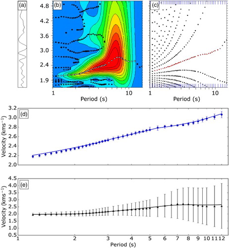
The CCF for path 16 annotated in Figure 1(a) is shown in Figure 3. The signal from time lags 0 to −120 s represents a dispersive surface wave travelling along path 16, from the Riverhead and Waiheke Island, and one travelling in the opposite direction for time lags 0 to +120 s. Note that the longer period signals (also higher amplitude in this case) generally arrive earlier than shorter period signals, illustrating frequency dependence in the wave speed. Asymmetry in the amplitude of the causal (0 to +120 s) and acausal (0 to −120 s) parts of the CCFs is an indication that ocean noise does not have a uniform azimuthal distribution. In our study area, ocean noise propagating east has comparatively high energy, resulting in the CCFs for interstation paths oriented east–west having the greatest asymmetry in amplitude. Figure 4(a) shows the folded CCF or symmetric component of the CCF in Figure 4(b) shows the group velocity estimates by period, over a coloured background representing spectral amplitudes. The highest energy band is 3 to 10 s. All CCFs contained dispersion information and we applied multiple filter techniques to the periods from 1 to 15 s. Figure 4(c). shows possible phase velocities by period. The frequency dependence of Rayleigh wave phase velocity is shown in Figure 4(d) which presents our picks from Figure 4(c) and the predicted dispersion curve for the final model for path 16. The frequency dependence of Rayleigh wave group velocity is shown in Figure 4(e) which presents our picks from Figure 4(b) and the predicted dispersion curve for our final model for path 16.

Figure 3. Cross-correlation function from 200 days of seismic records from seismometers along path 16 (Figure 1a) between stations at the Riverhead (RVAZ) and Waiheke Island (WIAZ).

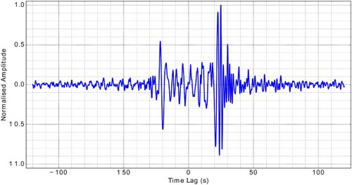
Figure 4. (a) Folded cross-correlation function from 200 days of seismic records from seismometers along path 16 (Figure 1a) between stations at the Riverhead (RVAZ) and Waiheke Island (WIAZ). B–E were computed from this CCF. (b) Group velocity by period, over a coloured background that corresponds to the spectral amplitudes (blue through red representing lowest to highest). The black markers represent estimates for the 10 largest amplitude envelopes. The white markers represent our picks. (c) Possible phase velocities by period. Solving for phase velocity introduces a 2πN uncertainty (each curve represents a different N value; Herrmann 1973). The red symbols mark our picks. (d) Frequency dependence of Rayleigh wave phase velocity. The solid lines are the predicted dispersion curve and error bars represent sampling errors. (e) Frequency dependence of Rayleigh wave group velocity obtained by multiple filter analysis. The black line is the predicted dispersion curve and the error bars were computed as if the travel-time were mis-measured by a single filter period.

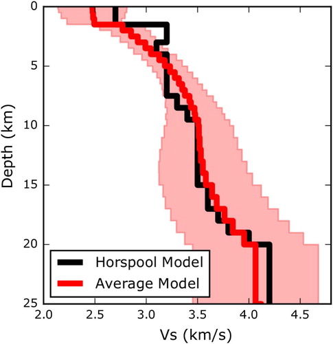
These curves are inverted with surf96 to obtain a 1D earth model that explains the observed dispersion. We inferred information about the shear-wave profile from the surface to c. 25 km depth from noise-generated surface waves between stations. The lower bound on the frequency content limited the sensitivity of these surface waves to 25 km. The average velocity model from this process agrees well with the velocity model from Horspool et al. (2006) for station MKAZ (Figure 5). The average model and the Horspool et al. (2006) model show an increasing velocity with depth, with an abrupt increase in velocity at 2 km, and a higher than average rate of increase between 15 and 20 km. The most notable differences are that the average model is smoother than the Horspool et al. (2006) model and has a higher rate of increasing velocity increase with depth between 2 and 8 km. The average model, however, largely supports the crustal part of the Horspool et al. (2006) model.

Figure 5. Average of 16 models from this study compared with a single model from Horspool et al. (2006). The boundaries of the pink region mark the standard deviation of the 16 models at each layer. The average model is the result of 16 cross-correlation functions. The Horspool et al. (2006) model was obtained by joint inversion of surface waves and receiver functions from the MKAZ broadband seismometer.

The standard deviation of the 16 1D models in each layer is larger, ranging from 0.17 to 0.65 km s⁻¹ (Figure 5) compared with the average standard error of the dispersion fit of models, which is 0.04 km s⁻¹, suggesting that the differences between models represent lateral variations in seismic velocity. The variability in the 1D models can be used for a preliminary geological interpretation of the AVF subsurface. At depths to 1.5 km, the models can be divided into a group with higher shear velocities and a group with lower shear velocities, with the lower velocities ranging between 2 and 2.5 km s⁻¹, and the higher velocities fitting into the broader range of 2.5–3.2 km s⁻¹ (Figure 6).

Figure 6. Seismic shear-wave velocity estimates for the top 1.5 km. Each model has four layers in the top 1.5 km and shows the average velocity that shear waves travel along each inter-station path at depths close to the surface. The numbers in the legend refer to paths mapped in Figure 7. Note the subdivision into a group with lower velocities and a group with higher velocities in comparison to the Horspool et al. 2006 model.

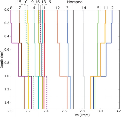
For the models at shallow levels (<1.5 km), the inter-station paths with high velocities tend to be concentrated in the eastern part of the study area, where the relatively dense terrigenous rocks of the Waipapa Terrane are exposed at the surface (Figure 7). Of these, paths 2, 11, 12 and 14 lie almost entirely in the exposed basement. Path 5 is an exception, having high shear-wave velocities but it is also similarly positioned to path 4 which has low shear-wave velocities. Inter-station paths with low velocities at shallow levels are dominant in the western part of the area where the basement sinks to lower levels and is covered by lower density Tertiary to recent sedimentary rocks, particularly, the Miocene Waitemata and Waitakere groups. The low-velocity materials are most conspicuous in and around the two harbours of Auckland, i.e. in the depression where the city is located and where low-density sedimentary rocks prevail.

Figure 7. Shallow structure (<1.5 km depth). Two different types of paths between pairs of seismic stations distinguished by line patterns. Solid lines indicate high velocities, dashed lines low velocities. Note the preponderance of high-velocity paths in the east and of low-velocity paths in the west. The geological map is modified after Kermode & Heron (1992).

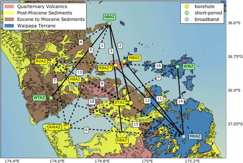
At deeper levels (>1.5 km depth) one group of models exhibits low-velocity zones (LVZ) at depths of 10–20 km (Figure 8), whereas the remaining models show shear-wave velocities that increase monotonically with depth (Figure 9). For these two groups, there is again a regional difference between the east and the west of the area (Figure 10), with paths modelling a LVZ predominating in the eastern half, while those with a monotonic increase are more common in the northwest. Stations RBAZ, MBAZ (Motutapu Island), WIAZ (Waiheke Island) and ETAZ (Tamaki) lie in the east and only participate in paths that model a LVZ. By contrast, stations KBAZ and RBAZ participate only in paths with a monotonic increase in velocity. We note that the latter two are the stations closest to or on the JMA, the expression of the subsurface location of the Dun Mountain Belt.

Figure 8. Seismic shear-wave velocity estimates from 0 to 25 km, for individual paths (the numbers in the legend refer to paths mapped in Figure 1a and Figure 10). These nine models show a low-velocity zone between 10 and 20 km.

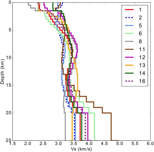
Figure 9. Seismic shear-wave velocity estimates from 0 to 25 km, for a specific path (the numbers in the legend refer to paths mapped in Figures 1a and 10). Note that in contrast to the models in Figure 8, these seven models show largely monotonic increases in velocity with depth.

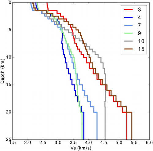
Figure 10. Deeper structures (>1.5 km depth). Two different types of paths between pairs of seismic stations distinguished by their line pattern. Solid lines indicate paths where shear velocities increase monotonically with depth, dashed lines indicate paths with low-velocity zones. Junction Magnetic Anomaly is shown using data from Eccles et al. 2005. Paths with low-velocity zones tend to be anchored in the east where Waipapa Terrane is dominant. Paths with monotonic velocity increases tend to prevail in the west where the Dun Mountain Belt exerts a greater influence.

An approximate tomographic model of the crust under the AVF is the result of interpolation of the 1D models shown in Figures 8 and 9 to 2D horizontal slices proceeding from near surface to depth (Figure 11). The following important features appear: (1) between 0–2 km depths, there are distinctly higher velocities in the northeast half, lower velocities in the southwest half, and a high-velocity spot in the southeast corner; (2) at 6 km deep, there is a zone of high velocity, also aligned northwest–southeast; and (3) a sub-rectangular area of relatively low velocity appears under the AVF down from c. 16 km and (4) a high-velocity body appears down from c. 12 km in the southwest sector.

Figure 11. A tomographic assemblage of lateral variations in shear-wave velocity cut into 2D slices in 2 km intervals descending to 24 km. Coastlines and surface trace of the Junction Magnetic Anomaly (JMA, dotted line) which represents the Dun Mountain Ophiolite Belt are both shown for reference.

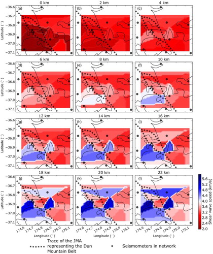
So far, there are only fragmentary indications of features representing the position and general trend of the Dun Mountain belt, the dominant tectonic feature of the region (e.g. Figure 11c–l).

Discussion

The agreement between the average of the 16 velocity models for individual station pairs and a model obtained by independent methods (Horspool et al. 2006) builds confidence in our shear-wave models for the AVF (Figure 5). Both the Horspool et al. (2006) model and our model have higher resolution than the P-wave models in Stern et al. (1987), Maunder (2001) and Ashenden et al. (2011), which have only two to three layers in the upper 25 km. At both shallow and deeper levels of the crust, two different groups of seismic models can be distinguished among the individual seismic models between station pairs. This encourages us to examine the patterns in more detail and to speculate how far the influence of geology may already be becoming apparent.

Our models penetrate with resolution to c. 25 km based on limited low-frequency content (Ensing 2015). Stern et al. (1987) estimated a Moho depth of 25 ± 2 km, whereas Horspool et al. (2006) found upper mantle velocities as shallow as 27–29 km in the Auckland region. This suggests that our models cover most of the crust, nearly reaching the Moho.

The estimates of impulse responses from ambient seismic noise in the Auckland region indicate that the AVF lies in a noise field (Figure 3) that is complex and varied. There is a broad range of wave periods in the noise signals (Figures 3 and 4) and noise sources are widely distributed. The azimuthal distribution of asymmetry in amplitude is in general agreement with those in Lin et al. (2007), but in Auckland, the greatest asymmetry in amplitude is for interstation paths oriented east–west (Ensing 2015), an orientation not represented in Auckland or Northland by Lin et al. (2007). It is likely that a portion of the asymmetry in the noise field may be explained by the difference in wave heights between the west and east coasts. Future work using multicomponent data may reveal even more about the azimuthal distribution of noise around Auckland. The periods of signals with the highest spectral amplitudes typically lie in the 3–10 s range (Figure 4b), which is consistent with other studies using ambient seismic noise (Ardhuin et al. 2011, 2015). This suggests that the seismic noise was primarily generated in shallow coastal areas where marine surface gravity waves interact with the ocean floor (Stehly et al. 2006; Yang & Ritzwoller 2008).

Some of the models in the group with monotonic velocity increase, such as those for paths 3 and 15 in Figure 9, show values that exceed those expected at depths shallower than 25 km, due to signal appearing in the CCFs from surface wave out of line with the inter-station paths (van Wijk et al. 2011). The future addition of cross-term CCFs should not only diminish this bias but also retrieve a greater frequency range in the signal (van Wijk et al. 2011; Haney et al. 2012).

Cover rocks

At depths to 1.5 km, a group of models with higher shear velocities can be distinguished from a group with lower velocities (Figure 6). Models with inter-station paths with high velocities are spatially correlated with the relatively dense terrigenous rocks of the Waipapa Terrane that are exposed at the surface (Figure 7). Paths with low velocities at shallow levels are dominant in the western part of the area (Figure 11a,b), where a deeper basement is covered by lower density Tertiary to Holocene sedimentary rocks, in particular, the Miocene Waitemata and Waitakere groups.

Murihiku and Waipapa terranes

Two of the three generalised tectonic units in the basement of the Auckland area (Figure 2), the Waipapa and the Murihiku terranes, are relatively similar in that they consist of terrigenous clastic sedimentary rocks and contain no, or very limited, oceanic material with higher densities. The eastward-skewed distribution of inter-station traces with a LVZ makes a causal link with the Waipapa Terrane reasonably likely (Figures 8 and 10). It is unclear what causes this low-velocity feature, but it may mark an especially shallow onset of the brittle/ductile transition in this part of the crust. Whether there is also a low-velocity anomaly contribution from the similar Murihiku Terrane is not yet discernible, but the fact that some inter-station lines with a LVZ cross the whole region (i.e. lines 1, 5, 6, 8, 13 and 16 in Figure 10) may be a hint in that direction. We do not consider this LVZ to be magma chamber-generated because geochemical analysis of volcanic deposits in the AVF find very little crustal contamination, point to magma sources that are down in the upper mantle (Huang et al. 1997; McGee et al. 2013), and are associated with a deeper LVZ at 70–90 km (Horspool et al. 2006). At this stage, we restrict ourselves to recognising that this low-velocity feature distinguishes areas of outcropping Waipapa Terrane and from areas we expect to see the Dun Mountain–Maitai Terrane (See below).

Dun Mountain–Maitai Terrane

The Dun Mountain–Maitai Terrane, in contrast to the Waipapa and the Murihiku terranes, is dominated by thick oceanic, mostly igneous crustal and mantle rocks, including the Dun Mountain belt, and can be expected to be geophysically different from the other two terranes. The western preponderance of traces with a monotonic increase in velocity (Figures 9 and 10) may indicate an influence of the oceanic rocks in the Dun Mountain–Maitai Terrane, for the following reasons: the steeply dipping part of the Dun Mountain–Maitai Terrane bisects our study area (Figure 11). It is modelled to form a syncline by resuming a sub-horizontal attitude towards the west, i.e. it is likely to be confined to the western part of the area (Figure 2). This may be supported by the position on or near the JMA of the two stations (KBAZ and RBAZ, Figure 11) that only participate in paths with monotonic velocity increase and therefore may be directly sampling the Dun Mountain–Maitai Terrane.

From c. 4 km depth (Figure 11c–l), a mass of higher velocity rocks inserts itself from the west and becomes increasingly prominent. It is interesting to note that this could be a signal from the sub-horizontal western limb of the syncline postulated for the configuration of the Dun Mountain–Maitai terrane (Figure 2). A subdivision into higher velocity rocks in the west and lower velocity rocks in the east becomes established, reflecting a dominant influence of the dense (fast) rocks of the Dun Mountain belt. At higher levels, this would be masked by a strong effect from the overlying lower density (slower) Murihiku Terrane material.

Auckland Volcanic Field

The very thin and discontinuous deposits of the AVF do not seem to impact on the velocity patterns. Lava flows would counteract the low velocities seen at shallow levels, whereas volcaniclastic deposits could contribute to or be neutral to them. The cause for the region of relatively lower velocities down from 10 km (Figure 11f) under Auckland City and roughly corresponding to the AVF footprint is yet unknown. As stated above, the nature of the AVF and its magma feeders does not allow us to postulate any crustal magma chambers. Alternative explanations could be a zone of thermal activity or alteration, a deeper basin filled with yet unknown lower density sedimentary rocks or a local volume of special low-density rocks within the Dun Mountain Belt.

Conclusions

The analysis of ambient seismic noise improves our understanding of the 3D crustal structure under the Auckland Volcanic Field. 1D seismic tomography has allowed us to make first-pass distinctions between geologic environments both at shallow and deeper levels. Shear-wave velocities in the top 1.5 km of the crust correlate with variations in surface geology, with lower velocities in areas dominated by low-density sedimentary deposits, and higher velocities in areas dominated by comparatively dense rocks. At greater depths, we are able to distinguish between domains primarily containing terrigenous sedimentary rocks and domains dominated by oceanic material. Paths along which Waipapa Terrane (relatively juvenile continental crust) are dominant typically show a crustal low-velocity anomaly, while velocities increase monotonically with depth for paths that go through the ophiolite belt of the Dun Mountain–Maitai Terrane (oceanic crust) that diagonally crosses the region and causes the JMA.

Future inclusion of multicomponent data and the additions of ray paths between stations is expected to improve resolution and penetration depth of these subsurface models.

Acknowledgements

We acknowledge support from DEVORA and the University of Auckland. We gratefully acknowledge technical help and advice from Robert Herrmann, Thomas Lecocq and Mark Chadwick. We thank Dr Jennifer Eccles for her help with the magnetic data. We also acknowledge the New Zealand GeoNet project and its sponsors EQC, GNS Science and LINZ. We thank Martha Savage and an anonymous reviewer for their helpful remarks. Associate editor: Associate Professor Andrew Gorman.

Disclosure statement

No potential conflict of interest was reported by the authors.

ORCID

J. X. Ensing http://orcid.org/0000-0001-9569-8832

K. van Wijk http://orcid.org/0000-0003-4994-8030

References

- Adams CJ, Mortimer N, Campbell HJ, Griffin WL. 2009. Age and isotopic characterisation of metasedimentary rocks from the Torlesse Supergroup and Waipapa group in the central North Island, New Zealand. New Zealand Journal of Geology and Geophysics. 52:149–170. doi: 10.1080/00288300909509883
- Ardhuin F, Gualtieri L, Stutzmann E. 2015. How ocean waves rock the earth: Two mechanisms explain microseisms with periods 3 to 300 s. Geophysical Research Letters. 42:765–772. doi: 10.1002/2014GL062782
- Ardhuin F, Stutzmann E, Schimmel M, Mangeney A. 2011. Ocean wave sources of seismic noise. Journal of Geophysical Research: Oceans. 116:1–21, article number C09004. doi: 10.1029/2011JC006952
- Ashenden CL, Lindsay JM, Sherburn S, Smith IE, Miller CA, Malin PE. 2011. Some challenges of monitoring a potentially active volcanic field in a large urban area: Auckland volcanic field, New Zealand. Natural Hazards. 59:507–528. doi: 10.1007/s11069-011-9773-0
- Bache F, Mortimer N, Sutherland R, Collot J, Rouillard P, Stagpoole V, Nicol A. 2014. Seismic stratigraphic record of transition from Mesozoic subduction to continental breakup in the Zealandia sector of eastern Gondwana. Gondwana Research. 26:1060–1078. doi: 10.1016/j.gr.2013.08.012
- Bebbington MS, Cronin SJ. 2011. Spatio-temporal hazard estimation in the Auckland volcanic field, New Zealand, with a new event-order model. Bulletin of Volcanology. 73:55–72. doi: 10.1007/s00445-010-0403-6
- Behr Y, Townend J, Bannister S, Savage M. 2010. Shear velocity structure of the Northland Peninsula, New Zealand, inferred from ambient noise correlations. Journal of Geophysical Research: Solid Earth. 115:1–12, article number B05309. doi: 10.1029/2009JB006737
- Behr Y, Townend J, Bannister S, Savage M. 2011. Crustal shear wave tomography of the Taupo volcanic zone, New Zealand, via ambient noise correlation between multiple three-component networks. Geochemistry, Geophysics. 12:1–18, article number Q03015.
- Behr Y, Townend J, Bowen M, Carter L, Gorman R, Brooks L, Bannister S. 2013. Source directionality of ambient seismic noise inferred from three-component beamforming. Journal of Geophysical Research: Solid Earth. 118:240–248.
- Briggs RM, Middleton MP, Nelson CS. 2004. Provenance history of a Late Triassic-Jurassic Gondwana margin forearc basin, Murihiku Terrane, North Island, New Zealand: Petrographic and geochemical constraints. New Zealand Journal of Geology and Geophysics. 47:589–602. doi: 10.1080/00288306.2004.9515078
- Camanni G, Alvarez-Marron J, Brown D, Ayala C, Wu Y, Hsieh H. 2016. The deep structure of south-central Taiwan illuminated by seismic tomography and earthquake hypocenter data. Tectonophysics. 679:235–245. doi: 10.1016/j.tecto.2015.09.016
- Cho KH, Herrmann RB, Ammon CJ, Lee K. 2007. Imaging the upper crust of the Korean Peninsula by surface-wave tomography. Bulletin of the Seismological Society of America. 97:198–207. doi: 10.1785/0120060096
- Cooley JW, Tukey JW. 1965. An algorithm for the machine calculation of complex Fourier series. Mathematics of Computation. 19:297. doi: 10.1090/S0025-5718-1965-0178586-1
- Daczko NR, Klepeis KA, Clarke GL. 2001. Evidence of Early Cretaceous collisional-style orogenesis in northern Fiordland, New Zealand and its effects on the evolution of the lower crust. Journal of Structural Geology. 23:693–713. doi: 10.1016/S0191-8141(00)00130-9
- Davy B. 2008. Marine seismic reflection profiles from the Waitemata-Whangaparoa region, Auckland. New Zealand Journal of Geology and Geophysics. 51:161–173. doi: 10.1080/00288300809509857
- Eccles J, Cassidy J, Locke C, Spörli K. 2005. Aeromagnetic imaging of the Dun Mountain ophiolite belt in northern New Zealand: Insight into the fine structure of a major SW Pacific terrane suture. Journal of The Geological Society. 162:723–735. doi: 10.1144/0016-764904-060
- Edbrooke SW, Mazengarb C, Stephenson W. 2003. Geology and geological hazards of the Auckland urban area, New Zealand. Quaternary International. 103:3–21. doi: 10.1016/S1040-6182(02)00129-5
- Ensing JX. 2015. Ambient Seismic Noise Tomography in the Auckland Volcanic Field. [Master’s thesis] Auckland, New Zealand: University of Auckland. Available from: http://hdl.handle.net/2292/27668
- GeoNet. 2001. GeoNet New Zealand Seismograph Network. GNS Science. doi: 10.21420/G2WC7M
- Gorman RM, Bryan KR, Laing AK. 2003. Wave hindcast for the New Zealand region: nearshore validation and coastal wave climate. New Zealand Journal of Marine and Freshwater Research. 37:567–588. doi: 10.1080/00288330.2003.9517190
- Haney MM, Mikesell TD, van Wijk K, Nakahara H. 2012. Extension of the spatial autocorrelation (SPAC) method to mixed-component correlations of surface waves. Geophysical Journal International. 191:189–206. doi: 10.1111/j.1365-246X.2012.05597.x
- Hatherton T, Sibson R. 1970. Junction magnetic anomaly north of Waikato river. New Zealand Journal of Geology and Geophysics. 13:655–662. doi: 10.1080/00288306.1970.10431336
- Hayward BW. 1993. The tempestuous 10 million year life of a double arc and intra-arc basin-New Zealand's Northland Basin in the Early Miocene. Sedimentary Basins of the World. 2:113–142.
- Hayward BW, Murdoch G, Maitland G. 2011. Volcanoes of Auckland: The essential guide. Auckland: Auckland University Press.
- Herrmann RB. 1973. Some aspects of band-pass filtering of surface waves. Bulletin of the Seismological Society of America. 63:663–671.
- Herrmann RB. 2013. Computer programs in seismology: An evolving tool for instruction and research. Seismological Research Letters. 84:1081–1088. doi: 10.1785/0220110096
- Horspool N, Savage M, Bannister S. 2006. Implications for intraplate volcanism and back-arc deformation in northwestern New Zealand, from joint inversion of receiver functions and surface waves. Geophysical Journal International. 166:1466–1483. doi: 10.1111/j.1365-246X.2006.03016.x
- Huang Y, Hawkesworth C, van Calsteren P, Smith I, Black P. 1997. Melt generation models for the Auckland volcanic field, New Zealand: constraints from U Th isotopes. Earth and Planetary Science Letters. 149:67–84.
- Kenny J, Lindsay J, Howe T. 2012. Post-Miocene faults in Auckland: Insights from borehole and topographic analysis. New Zealand Journal of Geology and Geophysics. 55:323–343. doi: 10.1080/00288306.2012.706618
- Kereszturi G, Cappello A, Ganci G, Procter J, Németh K, Del Negro C, Cronin SJ. 2014. Numerical simulation of basaltic lava flows in the Auckland volcanic field, New Zealand—implication for volcanic hazard assessment. Bulletin of Volcanology. 76:1–17, article number 879.
- Kermode LO, Heron DW. 1992. Geology of the Auckland urban area. Series: Institute of Geological and Nuclear Sciences Geological map 2. Lower Hutt, New Zealand: Institute of Geological and Nuclear Sciences Ltd. ISBN 0478070004.
- Larose E, Margerin L, Derode A, van Tiggelen B, Campillo M, Shapiro N, Paul A, Stehly L, Tanter M. 2006. Correlation of random wavefields: An interdisciplinary review. Geophysics. 71:SI11–SI21. doi: 10.1190/1.2213356
- Lecocq T, Caudron C, Brenguier F. 2014. MSNoise, a python package for monitoring seismic velocity changes using ambient seismic noise. Seismological Research Letters. 85:715–726. doi: 10.1785/0220130073
- Lin F, Moschetti MP, Ritzwoller MH. 2008. Surface wave tomography of the western united states from ambient seismic noise: Rayleigh and love wave phase velocity maps. Geophysical Journal International. 173:281–298. doi: 10.1111/j.1365-246X.2008.03720.x
- Lin F, Ritzwoller MH, Townend J, Bannister S, Savage MK. 2007. Ambient noise Rayleigh wave tomography of New Zealand. Geophysical Journal International. 170:649–666. doi: 10.1111/j.1365-246X.2007.03414.x
- Lindsay J, Leonard G, Smid E, Hayward B. 2011. Age of the Auckland volcanic field: A review of existing data. New Zealand Journal of Geology and Geophysics. 54:379–401. doi: 10.1080/00288306.2011.595805
- Maunder D. 2001. New Zealand seismological report 1999. Seismological Observatory Bulletin E-182, Institute of Geological & Nuclear Science. 7:2001.
- McGee LE, Smith IE, Millet M, Handley HK, Lindsay JM. 2013. Asthenospheric control of melting processes in a monogenetic basaltic system: A case study of the Auckland volcanic field, New Zealand. Journal of Petrology. 54:2125–2153, article number egt043.
- Mortimer N, Gans P, Palin J, Meffre S, Herzer R, Skinner D. 2010. Location and migration of Miocene–Quaternary volcanic arcs in the SW Pacific region. Journal of Volcanology and Geothermal Research. 190:1–10. doi: 10.1016/j.jvolgeores.2009.02.017
- Pyle ML, Wiens DA, Nyblade AA, Anandakrishnan S. 2010. Crustal structure of the Transantarctic Mountains near the Ross Sea from ambient seismic noise tomography. Journal of Geophysical Research: Solid Earth. 115:1–13, article number B11310.
- Saygin E, Kennett B. 2012. Crustal structure of Australia from ambient seismic noise tomography. Journal of Geophysical Research: Solid Earth. 117:1–15, article number B01304. doi: 10.1029/2011JB008403
- Shapiro NM, Campillo M. 2004. Emergence of broadband Rayleigh waves from correlations of the ambient seismic noise. Geophysical Research Letters. 31:1–4, article number L07614. doi: 10.1029/2004GL019491
- Shapiro NM, Campillo M, Stehly L, Ritzwoller MH. 2005. High-resolution surface-wave tomography from ambient seismic noise. Science. 307:1615–1618. doi: 10.1126/science.1108339
- Smith I, Blake S, Wilson C, Houghton B. 2008. Deep-seated fractionation during the rise of a small-volume basalt magma batch: Crater Hill, Auckland, New Zealand. Contributions to Mineralogy and Petrology. 155:511–527. doi: 10.1007/s00410-007-0255-z
- Snieder R. 2004. Extracting the Green’s function from the correlation of coda waves: A derivation based on stationary phase. Physical Review E. 69:1–8, article number 046610. doi: 10.1103/PhysRevE.69.046610
- Spörli KB, Aita Y, Gibson GW. 1989. Juxtaposition of Tethyan and non-Tethyan Mesozoic radiolarian faunas in melanges, Waipapa Terrane, North Island, New Zealand. Geology. 17:753–756. doi: 10.1130/0091-7613(1989)017<0753:JOTANT>2.3.CO;2
- Spörli KB, Black PM, Lindsay JM. 2015. Excavation of buried Dun Mountain–Maitai terrane ophiolite by volcanoes of the Auckland Volcanic field, New Zealand. New Zealand Journal of Geology and Geophysics. 58:229–243. doi: 10.1080/00288306.2015.1035285
- Stankiewicz J, Ryberg T, Haberland C, Natawidjaja D. 2010. Lake Toba volcano magma chamber imaged by ambient seismic noise tomography. Geophysical Research Letters. 37:1–5, article number L17306. doi: 10.1029/2010GL044211
- Stankiewicz J, Weber MH, Mohsen A, Hofstetter R. 2012. Dead Sea basin imaged by ambient seismic noise tomography. Journal of Asian Earth Sciences. 169:615–623.
- Stehly L, Campillo M, Shapiro NM. 2006. A study of the seismic noise from its long-range correlation properties. Journal of Geophysical Research: Solid Earth. 111:1–12, article number B10306. doi: 10.1029/2005JB004237
- Stern T, Smith E, Davey F, Muirhead K. 1987. Crustal and upper mantle structure of the northwestern North Island, New Zealand, from seismic refraction data. Geophysical Journal of the Royal Astronomical Society. 91:913–936. doi: 10.1111/j.1365-246X.1987.tb01674.x
- Sutherland R. 1999. Basement geology and tectonic development of the greater New Zealand region: an interpretation from regional magnetic data. Tectonophysics. 308:341–362. doi: 10.1016/S0040-1951(99)00108-0
- Tindle C, Murphy MJ. 1999. Microseisms and Ocean Wave Measurements. IEEE Journal of Oceanic Engineering. 24:112–115. doi: 10.1109/48.740159
- van Wijk K, Mikesell TD, Schulte-Pelkum V, Stachnik J. 2011. Estimating the Rayleigh-wave impulse response between seismic stations with the cross terms of the Green tensor. Geophysical Research Letters. 38:1–4, article number L16301. doi: 10.1029/2011GL047442
- Williams HA, Cassidy J, Locke CA, Spörli KB. 2006. Delineation of a large ultramafic massif embedded within a major SW Pacific suture using gravity methods. Tectonophysics. 424:119–133. doi: 10.1016/j.tecto.2006.07.009
- Yang Y, Ritzwoller MH. 2008. Characteristics of ambient seismic noise as a source for surface wave tomography. Geochemistry, Geophysics, Geosystems. 9:1–18, article number Q02008. doi: 10.1029/2007GC001814
- Yao H, van Der Hilst RD, Maarten V. 2006. Surface-wave array tomography in SE Tibet from ambient seismic noise and two-station analysis - I. Phase velocity maps. Geophysical Journal International. 166:732–744. doi: 10.1111/j.1365-246X.2006.03028.x
- Young M, Cayley R, McLean M, Rawlinson N, Arroucau P, Salmon M. 2013. Crustal structure of the east Gondwana margin in southeast Australia revealed by transdimensional ambient seismic noise tomography. Geophysical Research Letters. 40:4266–4271. doi: 10.1002/grl.50878