Gravity anomaly grids for the New Zealand region

ABSTRACT

We present 1 arc-minute Bouguer, Faye, free air and topography corrected gravity anomaly grids for the New Zealand region, 25°S to 60°S and 160°E to 170°W. The grids were compiled from existing terrestrial, marine and satellite altimetry-derived gravity data enhanced with new airborne gravimetry data that were acquired for improvement of the New Zealand vertical datum. The airborne data seamlessly cover onshore and offshore areas over New Zealand’s North, South and Stewart islands with a uniform flight line spacing of 10 km. All data were corrected for the gravitational effect of the Geodetic Reference System 1980 (GRS80) reference ellipsoid and tied to the International Gravity Standardization Net 1971 (I.G.S.N.71) gravity datum. The gravity anomaly data from all sources were combined using the method of least squares collocation with a three dimensional logarithmic covariance function. Terrain corrections for gravity anomaly grids were calculated using an 8 m digital elevation model for topography above sea level and a 250 m seafloor topography model.

KEYWORDS:

• Gravity data
• airborne gravity survey
• Bouguer anomaly
• Faye gravity anomaly
• free air anomaly
• least squares collocation

Introduction

The 2013 and 2014 New Zealand airborne gravity survey was undertaken as part of the New Zealand vertical datum improvement project (McCubbine 2016). The survey provided a uniform gravity dataset at intermediate-scale resolution (10 km) that covers all of the North, South and Stewart islands of New Zealand and the immediate offshore area. The dataset is particularly useful in remote and mountainous areas where there are few terrestrial observations, and along the coast where there are few shipboard observations and satellite-derived gravity tends to be unreliable, e.g. due large sea surface variability (Hwang and Hsu 2008) or radar backscatter from the land (Deng and Featherstone 2006).

Previous gravity anomaly maps of the New Zealand region have been based solely on terrestrial observations using portable gravity meters (Reilly 1972) or combinations of terrestrial, shipborne observations and satellite-derived gravity (Rose 1991; Anderson et al. 2010; Sandwell et al. 2014). Acquisition of the airborne gravity provides an opportunity to combine all available gravity data (terrestrial, shipboard, airborne and satellite) and generate new gravity anomaly maps. A significant advantage of the new maps over their predecessors is that for the first time they are based on airborne gravity observations which seamlessly cover onshore and offshore areas of New Zealand.

As part of the vertical datum improvement project, the airborne gravity data were combined with existing terrestrial, marine and satellite altimetry gravity data to provide a grid suitable for geoid modelling. Data reduction entailed the determination of gravity anomalies by mathematical removal of the topographic masses outside the geoid (Heiskanen and Moritz 1967), i.e. correcting for the topography above mean sea level. To make the anomaly data useful to a wider audience, a grid of seafloor bathymetry was compiled and used to correct for topography below mean sea level and to then calculate the Bouguer anomaly for the complete area presented here.

This paper describes the data reduction to gravity anomalies and the method used to combine the different data sets. Bouguer, Faye, free air and topography corrected gravity anomaly grids derived from the combined data sets are presented here as 1 arc-minute resolution grids in the geographical region 25°S to 60°S and 160°E to 170°W. The gravity anomaly grids are publically available and can be used for regional geophysical and geological studies of the New Zealand region. The gravity units of the grids used throughout this paper are mGal (1 mGal = 10 µN/kg).

Data

Gravity correction formulas

The following formulas have been used to reduce the gravity data sets to gravity anomalies for the gridding process and are referenced in the subsequent text.

1. The ellipsoidal gravity effect(1) where,  = 9.7803267715 m/s² is the gravity at the equator, is the normal gravity constant and is the first eccentricity squared (where and are the semi-major and semi-minor axes of the GRS80 reference ellipsoid) and is the latitude (Moritz 1980).

2. The second order free air effect

   where , is the ratio between the gravitational and centrifugal forces at the equator and is the normal orthometric height in metres (Heiskanen and Moritz 1967).

3. The effect of a flat ‘slab’ of topography with height extending infinitely in the horizontal direction (commonly termed the Bouguer slab)(3) where is the rock density (taken to be 2.67 Mg/m³) and is the normal–orthometric height in metres above mean sea level.

4. The effect of topography variations from an observation point, a terrain correction that accounts for missing mass below the top of the Bouguer slab and additional mass above the Bouguer slab out to a defined radius of 120 km, beyond which the terrain effects are considered negligible,

   (4) withIn equation (4), is the difference between the height of the observation point and the height of the piece of topography being corrected for, is the spatial domain the terrain corrections are computed over, is the distance from the observation point to closest corner of the portion of topography being corrected for, and similarly is the distance to the corner furthest away, and finally is the horizontal resolution of the digital elevation model.

   This terrain correction uses a prism method, analogous to taking a segment of the effect of an annulus of topography given by Hammer’s (1939) formula. This formula is computationally easier than the more commonly used Nagy (1966) prism method and conservatively returns terrain corrections 10 times faster with almost identical results.

5. The gravitational effect of topography (i.e. similar to the combined effect of the Bouguer slab and the terrain correction). When a gravity observation is made above the surface of the Earth (as in the case of airborne gravity) it can be computed using a similar formula to that of equation (4):(5)

   where H is the height at the computation point and H′ is the height at the roving point over the summation.

6. To obtain a full Bouguer gravity anomaly the gravitational effect of seawater is replaced with the gravitational effect of rock. For the data onshore, a correction is given by equation (5) where is the observation height (> 0) is the ocean depth and  Mg/m³ (i.e. seawater density minus rock density). For data at sea, a Bouguer slab correction is added with  Mg/m³ and (> 0) the depth to the ocean floor. Then a correction is added of the form of equation (5) where (> 0) is the ocean depth at the computation point and is the ocean depth for an element in being corrected for minus the computation point depth. This correction is denoted here as .

Terrestrial gravity

GNS Science maintains a database of terrestrial gravity observations that have been made at c. 40,000 locations across New Zealand since the 1940s. Observations were made by several different institutions with various gravimeters. Most of the observations have been made with Lacoste and Romberg D and G relative gravity meters. All gravity data are tied to the New Zealand primary gravity network (Robertson and Reilly 1960) and referenced to the I.G.S.N.71 gravity datum (Morelli 1974). In general, the derived absolute gravity values from repeat relative gravity observations have an estimated accuracy of c. 0.1 mGal. The spatial density of observations varies across North, South and Stewart islands. In remote areas of rough topography, such as the central South Island, the gravity observations are sparse (> 10 km apart), whereas in areas of particular scientific interest (e.g. the Taupo Volcanic Zone) observations are on average < 1 km apart.

The original gravity values, , in the GNS Science database were reprocessed and reduced to topography corrected gravity anomalies (Figure 1) by calculating,(6) This was performed to ensure consistency in the formulas and digital elevation models used. A national 8 m digital elevation model (DEM) was used to calculate terrain corrections to account for the gravitational effect of topography above mean sea level out to a radius of 120 km (Anon 2012). Beyond 120 km it was assumed the gravitational effect of topography was negligible.

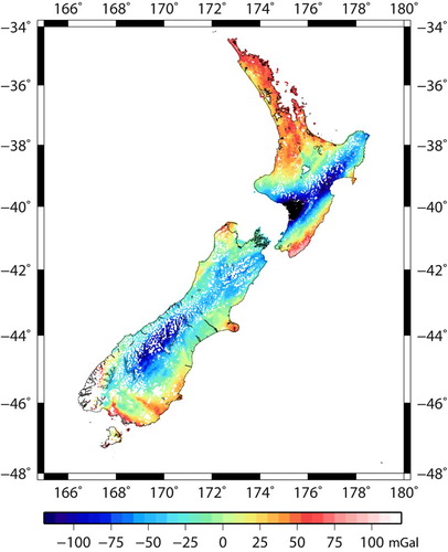
Figure 1. Terrestrial topography corrected gravity anomalies (mGal) over New Zealand’s North, South and Stewart islands. The point wise measurements shown as dots coloured by value.

Near zone (to 170 m) recomputed terrain corrections were carefully compared with existing near zone terrain corrections in the database that were estimated from field observations of the topography. The comparison highlighted discrepancies in calculating near zone terrain effects using the DEM, particularly in mountainous regions where miss-locating the gravity observation site has a large impact on the estimated terrain correction value. The DEM-derived terrain corrections were only used for the near zone where the existing terrain corrections were large (> 0.1 mGal) and DEM-derived terrain corrections were small (< 0.1 mGal), with the differences being attributed to over estimating variations of the terrain in the field.

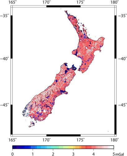
The most common source of errors in the terrestrial gravity anomaly data are inaccurate height measurements at gravity observation locations. In many cases, heights were determined by barometric levelling with a typical accuracy of ± 5 m (Reilly and Woodward 1971). The height discrepancies have been estimated by comparing the recorded heights in the database to those determined from the 8 m DEM and have been translated into mGal by calculating the propagated effect on the free air and Bouguer slab corrections. Overall, the estimated error for terrestrial data is c. 3.5 mGal, with patches of 0.5 and 0.02 mGal where there are highly accurate heights, such as those determined on survey benchmarks (Figure 2).

Figure 2. Terrestrial topography corrected gravity anomalies error standard deviations (mGal) estimated by propagating height uncertainties into the Bouguer and free air corrections. The error estimates are shown as dots coloured by value.

Airborne gravity

A New Zealand airborne gravity survey, conducted between September 2013 and June 2014, covered New Zealand’s North and South and Stewart islands with 203 fight lines, typically spaced 10 km apart. A LaCoste and Romberg dynamic gravimeter (model number S-80) was used for the airborne data collection from a twin-engine Piper Chieftain aircraft.

The lines were chosen to be as long as possible to avoid unnecessary aircraft turns. Each line was flown as close as possible to a constant altitude that best suited the topography (typically between 2000 and 4000 m) and a near constant speed of 130 knots (240 km/h). Measurements were made by the gravimeter at a rate of 1 Hz so that data points were acquired approximately every 65 m. All the observation data were initially reduced with the following eight steps (following Olesen 2002):

1. Relative gravity measurements were calculated from the raw signal of the gravimeter for all readings.

2. The constant , the ‘still’ relative gravity measurement for the S-80 meter and , the absolute gravity value (I.G.S.N.71 gravity datum) where the ‘still’ data were recorded, were specified for data along each flight line.

3. Vertical accelerations, for each entry in the GPS data were determined and used to synchronise the relative gravity measurements , with GPS data in the time domain.

4. The tilt correction was determined from the gravimeter accelerometer and cross/along track GPS data for each data point (Peters & Brozena 1995).

5. The Eötvos effect (Harlan 1968), ellipsoidal absolute gravity effect, and the second order free air effect , were determined for each data point.

6. The free air anomaly data, were then calculated using,(7)

7. The gravitational effect of the topography above mean sea level was then determined from a 64 m digital elevation model out to a radius of 120 km from each observation point. Beyond 120 km it was assumed the gravitational effect of topography was negligible. The topography corrected anomaly, at each data point was then determined by,(8)

8. The along-track topography corrected anomalies were then low-pass filtered to remove high-frequency noise. This was done using a Gaussian filter. The filter length was optimised to be 120 s by minimising the difference at flight line cross-over points.

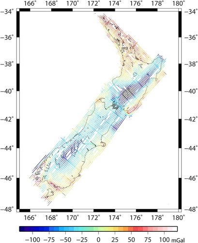
A second stage of processing was subsequently performed to obtain the final topography-corrected gravity anomalies along each flight line (Figure 3). Flying conditions were turbulent during some of the data collection and the gravimeter was not suited to measuring such extreme forces which resulted in erroneous sections of data, characterised as large spikes. These data were identified by comparing the along track data to neighbouring flight lines and to global Earth Gravitational Model 2008 (EGM2008) (Pavlis et al. 2012), and subsequently removed. In total, c. 7% of the data needed to be removed.

Figure 3. Airborne topography corrected gravity anomaly data (mGal) shown along each flight line coloured by value. Data which has been removed can be seen by the white space along the tracks and amounts to around 7% of the total data set.

The accuracy of the airborne gravity data is estimated to be c. 3 mGal and was assessed by two key methods.

1. The cross-over error: the difference between Bouguer gravity anomaly values at flight line intersection points. After accounting for track biases and varying flight line elevations the standard deviation of the cross-over differences was 5.9 mGal.

2. Repeated flights along two flight lines, one on the North Island and one on the South Island, demonstrated a repeatability of 2.2 and 2.5 mGal, respectively. Terrestrial gravity data were also obtained along these flight lines at ground level and had an agreement of 2.1 mGal standard deviation for the North Island airborne data and 3.3 mGal for the South Island.

The cross-over error is particularly sensitive to the type of gravity anomaly (free air or Bouguer), the along track filter length and the relative difference in flight line elevations (due to the attenuating effect of upward continuation). These systematic effects increase the cross-over error and are difficult to account for analytically. For these reasons we consider the cross-over error to provide the least accurate assessment of the data.

Finally, a bias correction was determined for each flight line. Potential sources of the bias include insufficiently accurate gravimeter still readings, GPS height errors, gravimeter operational errors and tilt correction uncertainties. The biases were estimated for each flight line by subtracting the free air anomaly determined from the EGM2008 global gravity model from the airborne topography corrected anomaly data, restoring the effect of topography filtered to a 9 km wavelength (similar to the minimum wavelength in EGM2008), fitting a three-dimensional logarithmic covariance function (Forsberg 1987) to the residual signal, and then solving equation (9) (Reilly 1979).(9) is an M length vector of the biases for each flight line, where M is the number of separate lines of data in the survey. These values should be subtracted from the line data so that it becomes ‘bias free’. The matrix is a covariance matrix that describes the spatially correlated signal in the residual gravity data with entries determined by the fitted covariance function; is a covariance matrix that describes the noise in the residual gravity observations (estimated to have a standard deviation of 3 mGal). describes which bias element each residual gravity observation will contribute to in the solution.

The inclusion of matrices and ensures the spatially correlated residual gravity signal and signal noise modelled by do not contribute to the determined biases. The method described above to compute flight line biases is better than estimating a mean offset from EGM2008 for each flight line because it takes into consideration the correlated signal between separate flight lines, and is better constrained than the standard approach of line bias estimation from flight line intersection discrepancies.

Shipborne gravity

Marine gravity observations have been collected in the New Zealand region for more than 50 years. Most of the data are publically available from GNS Science, the US National Oceanic and Atmospheric Administration (NOAA) geophysical data centre and Geoscience Australia (GA). More than 2 million individual observations collected along-track by numerous research vessels were accessed.

The data have previously been reduced to free air anomalies with respect to the GRS80 reference ellipsoid and cross-over adjusted to remove potential offsets between separate gravity surveys (Amos et al. 2005). The data were also further cleaned by removing obviously anomalous data, by examining the fourth-differences along each profile to highlight spikes and investigating further statistical outliers interactively, and then using a manual judgement to determine if the outliers should be removed. The cross-over error was evaluated to have a standard deviation of 2 mGal (Table 1), this figure is the assumed accuracy of the data.

Table 1. Cross-over statistics of the shipborne gravity data.

Source	Number of cross-overs	Max	Min	Mean	STD
NZ UNCLOS project	345	79.7	0	7.6	12.9
GNS Science	57,512	271.3	0	2.5	7.6
NOAA	971,988	236.1	0	0.7	0.7
GA	36,271	52.6	0	1.6	2.7
All data	1,069,289	271.3	0	0.8	2

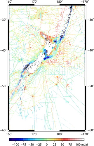
Terrain corrections were determined for the shipborne data from a 64 m digital elevation model accounting for the gravitational effect of topography above mean sea level within 120 km of the observation point. These were added to the free air anomalies to obtain shipborne topography corrected anomaly data (Figure 4).

Figure 4. Shipborne topography corrected gravity anomaly data (mGal) shown as dots coloured by value over the region 25°S to 60°S and 160°E to 170°W.

Satellite gravity

The satellite marine gravity anomaly grid (at 1 arc-minute) released in 2014 by Sandwell et al. (2014) was obtained from http://topex.ucsd.edu/cgibin/getdata.cgi (accessed September 2015). The grid is based on data from CryoSat-2 and Jason-1 augmented with older altimeter data from Geosat and ERS-1 satellites. The altimeter-derived gravity field is estimated to be accurate to 2 mGal.

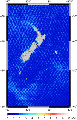
The gravity data over the land come from EGM2008 and were masked from this data set, so that only the altimetry-based data are used in the gridding (Figure 5). These gravity data are accompanied with a gridded map of errors (Figure 6) which are typically around 1–2 mGal over the open ocean. However, in shallow coastal regions these errors increase up to 50 mGal. The low accuracy in the shallow coastal zone is attributed predominately to sea surface variability (Hwang and Hsu 2008) which makes the mean sea surface hard to predict from altimeter observations.

Figure 5. Grid of Sandwell et al. (2014) satellite altimetry-derived gravity anomaly (mGal) corrected for topography (masked on shore) over the region 25°S to 60°S and 160°E to 170°W.

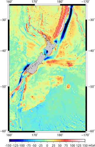
Figure 6. Grid of Sandwell et al. (2014) satellite altimetry-derived gravity anomaly error standard deviation (mGal) (masked on shore) over the region 25°S to 60°S and 160°E to 170°W. The error values are larger in coastal regions.

As with the shipborne data, terrain corrections were computed at each gravity anomaly data point to obtain gravity anomaly values corrected for the gravitational effect of topography above mean sea level within 120 km. For this correction a 1 arc-minute grid of topography heights was used to introduce high-frequency signals not captured by the 1 arc-minute resolution of the free air anomaly.

Combining and gridding data

The four separate gravity anomaly datasets have been augmented and gridded with the method of least squares collocation using the following process.

1. For all four data sets, residual gravity anomalies, , were obtained from the Bouguer gravity anomalies by subtracting the GOCE direct 5 (Bruinsma et al. 2013) global gravity anomaly model and adding the gravitational effect of the 8 m DEM filtered to a 77 km wavelength (approximately the minimum wavelength in the GOCE direct 5 global gravity model).

2. , and parameters of the logarithmic covariance function (Forsberg 1987) with the form(10) withwere fitted to the empirical spatial covariances of the full set of residual gravity anomalies .

3. The residual gravity signal was then interpolated at the locations specified by a grid of 1 arc-minute block averaged topographic heights by solving(11)

Here, is the interpolated gravity signal, is the variance–covariance matrix of the interpolated signal and the residual gravity observations (determined by equation 10), is the variance–covariance matrix of the residual gravity observations with themselves and is the variance–covariance matrix of the residual gravity signal noise.

For the residual gravity signal corresponding to the terrestrial gravity observations, the corresponding entries in on the diagonal are determined by the estimated gravity anomaly accuracy standard deviations (Figure 2) squared and zero for the off diagonal entries.

For the shipborne data, the entries in on the diagonal were set equal to 4 mGal², in line with the accuracy assesment, and are zero for the off diagonal entries. Similarly, for the satellite data, the entries in on the diagonal were set equal to the estimated standard deviations (Figure 6) squared as specified by the accompanying error map and again the off diagonal terms were set to zero.

Entries in for the airborne data were set equal to 9 mGal² on the diagonal and entries on the off diagonal terms were determined by equation (12) if the measurements were made along the same flight line and zero otherwise.(12) This ensures the along-track filter applied to the airborne data does not contaminate the gridded signal, since it causes errors along the flight lines to be correlated.

• (4) The GOCE direct 5 gravity anomaly was restored to the gridded residual signal and the effect of the 77 km wavelength filtered topography was subtracted to obtain a final gridded topography corrected gravity anomaly (Figure 7).

• (5) Using equation (13), the propogated effect of the residual gravity noise and spatial density can also be determined at each interpolated point from the values on the diagonal of the matrix ,(13)

The square root of these values has been taken to obtain gridded standard deviation estimates (Figure 8).

Figure 7. One arc-minute grid of airborne, terrestrial, shipborne and satellite altimetry-derived topography corrected anomaly data combined by least squares collocation over the region 25°S to 60°S and 160°E to 170°W. This shows the strength of the Earth’s gravity minus the gravitational effect of topography and an Earth approximating ellipsoid.

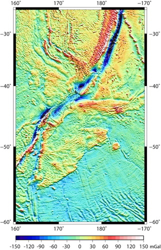
Figure 8. Gridded gravity anomaly error standard deviations (mGal) propagated from the airborne, terrestrial shipborne and satellite altimetry measurement errors by least squares collocation.

Restoring the effect of topography

Faye anomaly

The use of gravity anomaly data for gravimetric quasigeoid modelling necessitates the generation of a Faye anomaly grid. This is easiest to obtain by restoring the Bouguer slab effect to the topography corrected gravity anomalies.The Faye anomaly is the free air anomaly plus the terrain correction term or alternatively the topography corrected anomaly plus the effect of a Bouguer slab term, . To obtain the Faye anomaly over land areas the topographic grid was block averaged to 1 arc-minute and multiplied by the Bouguer slab factor 0.1119 mGal/m and added to the gridded topography corrected anomaly grid (Figure 9).

Figure 9. One arc-minute grid Faye anomalies over the region 25°S to 60°S and 160°E to 170°W showing the strength of the Earth’s gravity minus the gravitational effect of an Earth approximating ellipsoid and the effect of topography relative to the topographic height at each grid point.

Free air anomaly

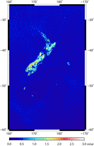
To obtain the free air anomaly, the 1 arc-minute block averaged topography was used to determine terrain corrections out to 120 km from each grid point. These were computed using the fast Fourier method (equation 14) which is appropriate because the east–west and north–south gradients of the 1 arc-minute DEM do not exceed 45° (Kirby and Featherstone 2001) (Table 2).(14) where is the 2D Fourier transformation operator, is the Euclidean distance between the computation point and points on the topograhpic grid H and (15) is the kernel weighting function with the resolution of the grid (Kirby and Featherstone 1999). Subtracting from the gridded Faye anomaly produces a free air anomaly grid (Figure 10).

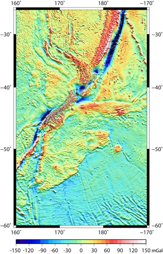
Figure 10. One arc-minute grid of free air anomalies (mGal) over the region 25°S to 60°S and 160°E to 170°W showing the strength of the Earth’s gravity minus the gravitational effect of an Earth approximating ellipsoid.

Table 2. Gradient summary statistics of the 1 arc-minute block averaged topography.

degrees	Min	Max	Mean	SD
East–west gradient in degrees	−41.8925	42.4410	0.0001	1.0303
North–south gradient in degrees	−30.0216	30.5869	−0.0001	0.7706

Bouguer anomaly—replacing the gravitational effect of seawater with rock

To make the data useful to a wider audience, the final 1 arc-minute grid of Bouguer gravity anomalies for the whole region has been obtained by employing an additional processing step using seafloor topographic data. The gravitational effect of the seawater was replaced with the gravitational effect of rock using a density contrast of 1.64 Mg/m³ to compute and adding it to the topography corrected gridded gravity anomaly (Figure 11). was computed using 1 arc-minute bathymetric depths derived from Mitchell et al. (2012) and GEBCO_2014 (version 20150318, http://www.gebco.net) grids of New Zealand regional bathymetry.

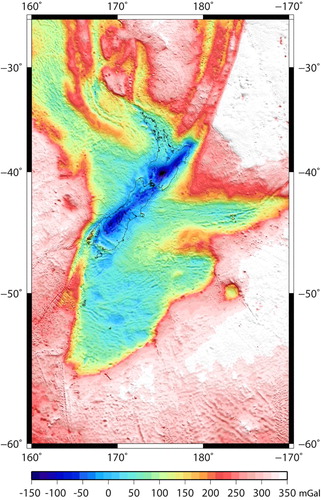
Figure 11. One arc-minute grid of Bouguer anomalies (mGal) over the region 25°S to 60°S and 160°E to 170°W. This shows the strength of the Earth’s gravity minus the gravitational effect of an Earth approximating ellipsoid and the topography above mean sea level and replacing the gravitational effect of seawater with the effect of rock with density 2.67 Mg/m³.

Discussion

Gravity field maps have been publically released at global (e.g. EGM2008 by Pavlis et al. 2012, Eigen-6C4 by Förste et al. 2014 Sandwell et al. 2014) and national-scale (e.g. for New Zealand by Reilly 1972 and Australia by Tracey et al. 2008). It is becoming more frequent for maps at regional and national scales to incorporate airborne gravity data as has been done for the grids presented here (e.g. Taiwan, Hwang et al. 2007; South Korea, Bae et al. 2012; Nepal, Forsberg et al. 2014; and the GRAV-D data over the Great Lakes region, Li et al. 2016). The new gravity grids covering the New Zealand region have been generated from four separate and independent datasets to create the most comprehensive gravity anomaly grids to date. Some 748,032 airborne data points, 1,069,289 shipborne observations and c. 40,000 terrestrial gravity observations have been combined with 1 arc-minute gridded satellite-derived gravity data points in the compilation. The final gravity grids and accompanying propagated error grid have optimally combined these data with a careful consideration of observation errors. Moreover, the use of a 3D logarithmic covariance function allows the airborne data to be gridded at the surface of the Earth while simultaneously being combined with the other data and so it avoids an explicit downward continuation.

The off diagonal elements in the noise matrix N for the airborne data are of particular importance. There are c. 15 airborne observations for every terrestrial observation; however, the errors in the airborne data are not independent due to the along track filtering. Without including the diagonal noise matrix terms, the number of the airborne observations overwhelmed the contributions of the terrestrial gravity observations in the least squares collocation procedure.

The final gravity grids were computed using all available terrestrial gravity observations and consequently the onshore data of the satellite altimetry-derived gravity anomaly were removed since they are based on a 10 km grid of terrestrial gravity measurements. In addition, the contribution of erroneous coastal gravity anomaly data in the satellite altimetry-derived gravity is heavily suppressed in the final grid by using the satellite dataset’s accompanying error map.

The gravity anomaly grids presented here were initially developed for quasigeoid modelling over New Zealand, but have been adapted to be used for more general geophysical research. For example, investigating crustal structure, or to help identify areas where higher resolution gravity data might be of interest for local geological investigations and mineral exploration. Although the gravity anomaly grids presented here are band limited to 1 arc-minute. In many regions across New Zealand the spatial data density is substantially greater. For this reason, there is scope for higher resolution grids to be produced in the future.

Acknowledgements

The authors thank LINZ, GNS Science, and Victoria University of Wellington for supporting this work. We thank Andrew Gorman and anonymous reviewers for making helpful suggestions to improve the manuscript. All gravity grids discussed here are available at http://www.gns.cri.nz/Home/Products/Databases

Disclosure statement

No potential conflict of interest was reported by the authors.

Additional information

Funding

Funding for the airborne gravity survey was provided by LINZ vertical datum improvement project. This work was also supported by GNS Science [Strategic Development Fund project S47].

References

- Amos MJ, Featherstone WE, Brett J. 2005. Crossover adjustment of New Zealand marine gravity data, and comparisons with satellite altimetry and global geopotential models. In: Gravity, geoid and space missions. Volume 129. IAG Symposia Series, Berlin (Germany): Springer; p. 266–271.
- Andersen OB. 2010. The DTU10 gravity field and mean sea surface 2010. Second international symposium of the gravity field of the Earth (IGFS2), Fairbanks, Alaska. http://www.space.dtu.dk/english/Research/Scientific_data_and_models/Global_Marine_Gravity_Field
- Anon. 2012. NZ 8m digital elevation model (2012). Wellington: LINZ data service, Land Information NZ; [accessed 2016]. https://data.linz.govt.nz/layer/1768-nz-8m-digital-elevation-model-2012/.
- Bae TS, Lee J, Kwon JH, Hong C. 2012. Update of the precision geoid determination in Korea. Geophysical Prospecting. 60(3):555–571. doi: 10.1111/j.1365-2478.2011.01017.x
- Bruinsma S, Foerste C, Abrikosov O, Marty JC, Rio MH, Mulet S, Bonvalot S. 2013. The new ESA satellite-only gravity field model via the direct approach. Geophysical Research Letters. 40:3607–3612. doi: 10.1002/grl.50716
- Deng X, Featherstone WE. 2006. A coastal retracking system for satellite radar altimeter waveforms: application to ERS-2 around Australia. Journal of Geophysical Research: Oceans. 111:C06012. doi: 10.1029/2005JC003039
- Forsberg R. 1987. A new covariance model for inertial gravimetry and gradiometry. Journal of Geophysical Research. 92:1305–1310. doi: 10.1029/JB092iB02p01305
- Forsberg R, Olesen AV, Einarsson I, Manandhar N, Shreshta K. 2014. Geoid of Nepal from airborne gravity survey. In: Rizos C, Willis P, editors. Earth on the edge: science for a sustainable planet: earth on the edge: science for a sustainable planet earth on the edge: science for a sustainable planet proceedings of the IAG general assembly, Melbourne, Australia; June 28 -July 2, 2011. Melbourne, Australia: Springer. pp. 521–527. (International Association of Geodesy Symposia, Vol. 139).
- Förste C, Bruinsma SL, Abrikosov O, Lemoine J-M, Marty JC, Flechtner F, Balmino G, Barthelmes F, Biancale R. 2014. EIGEN-6C4 the latest combined global gravity field model including GOCE data up to degree and order 2190 of GFZ Potsdam and GRGS Toulouse. GFZ Data Services. http://doi.org/10.5880/icgem.2015.1
- Hammer S. 1939. Terrain corrections for gravimeter stations. Geophysics. 4(3):184–194. doi: 10.1190/1.1440495
- Harlan RB. 1968. Eotvos corrections for airborne gravimetry. Journal of Geophysical Research. 73:4675–4679. doi: 10.1029/JB073i014p04675
- Heiskanen WA, Moritz H. 1967. Physical geodesy. San Francisco (USA): W.H. Freeman and Company; p. 364.
- Hwang C, Hsiao YS, Shih HC, Yang M, Chen KH, Forsberg R, Olesen AV. 2007. Geodetic and geophysical results from a Taiwan airborne gravity survey: data reduction and accuracy assessment. Journal of Geophysical Research: Solid Earth. 112:B04407. doi: 10.1029/2005JB004220
- Hwang C, Hsu H. 2008. Shallow-water gravity anomalies from satellite altimetry: case studies in the East China Sea and Taiwan Strait. Journal of the Chinese Institute of Engineers. 31(5):841–851. doi:10.1080/02533839.2008.9671437
- Kirby JF, Featherstone WE. 1999. Terrain correcting Australian gravity observations using the national digital elevation model and the fast Fourier transform. Australian Journal of Earth Sciences. 46(4):555–562. doi: 10.1046/j.1440-0952.1999.00731.x
- Kirby JF, Featherstone WE. 2001. Anomalously large gradients in the GEODATA 9 SECOND Digital Elevation Model of Australia, and their effects on gravimetric terrain corrections. Cartography. 30(1):1–10. doi: 10.1080/00690805.2001.9714131
- Li X, Crowley JW, Holmes SA, Wang YM. 2016. The contribution of the GRAV-D airborne gravity to geoid determination in the Great Lakes region. Geophysical Research Letters. 43(9):4358–4365. doi: 10.1002/2016GL068374
- McCubbine J. 2016. Airborne gravity across New Zealand – for an improved vertical datum [dissertation]. PhD Thesis. Victoria University of Wellington 2016.
- Mitchell JS, Mackay KA, Neil HL, Mackay EJ, Pallentin A, Notman P. 2012. Undersea New Zealand, 1:5,000,000. NIWA Chart, Miscellaneous Series No. 92. Wellington: National Institute of Water and Atmospheric Research.
- Morelli C. 1974. International gravity standardization net 1971 (I.G.S.N.71). International Association of Geodesy Special Publication no. 4, p. 194.
- Moritz H. 1980. Geodetic reference system 1980. Bulletin Godsique. 54(3):395–405. doi: 10.1007/BF02521480
- Nagy D. 1966. The gravitational attraction of a right angular prism. Geophysics. 31(2):362–371. doi: 10.1190/1.1439779
- Olesen AV. 2002. Improved airborne scalar gravimetry for regional gravity field mapping and geoid determination [dissertation]. PhD Thesis. University of Copenhagen.
- Pavlis NK, Holmes SA, Kenyon SC, Factor JK. 2012. The development and evaluation of the Earth Gravitational Model 2008 (EGM2008). Journal of Geophysical Research: Solid Earth. 117:B04406. doi: 10.1029/2011JB008916
- Peters MF, Brozena JM. 1995. Methods to improve existing shipboard gravimeters for airborne gravimetry. In: Schwartz KP, Brozena JM, Hein GW, editors. IAG symposium on airborne gravity field determination. Calgary, Boulder (CO): IUGG XXI General Assembly; p. 39–45.
- Reilly WI. 1972. New Zealand gravity map series. New Zealand Journal of Geology and Geophysics. 15:3–15. doi: 10.1080/00288306.1972.10423942
- Reilly WI. 1979. Mapping the local geometry of the earth’s gravity field. Report No.143. Geophysics Division, Department of Scientific and Industrial Research New Zealand.
- Reilly WI, Woodward DJ. 1971. Adjustment of observations in barometric levelling. New Zealand Journal of Geology and Geophysics. 14:293–298. doi: 10.1080/00288306.1971.10421927
- Robertson EI, Reilly WI. 1960. The New Zealand primary gravity network. New Zealand Journal of Geology and Geophysics. 3:41–68. doi: 10.1080/00288306.1960.10423143
- Rose K. 1991. Gravity anomaly map, Oceanic Series 1:1,000,000, Cook. Wellington: DSIR Geology & Geophysics.
- Sandwell DT, Muller RD, Smith WHF, Garcia E, Francis R. 2014. New global marine gravity model from CryoSat-2 and Jason-1 reveals buried tectonic structure. Science. 346(6205):65–67. doi:10.1126/science.1258213,2014
- Tracey R, Bacchin M, Wynne P. 2008. AGD07: a new absolute gravity datum for Australian gravity and new standards for the Australian National Gravity Database. ASEG Extended Abstracts 2007: 19th Geophysical Conference; p. 1–3. http://www.publish.csiro.au/EX/pdf/ASEG2007ab149.